Generalized Direct Sampling for Hierarchical Bayesian Models

Abstract

We develop a new method to sample from posterior distributions in hierarchical models without using Markov chain Monte Carlo. This method, which is a variant of importance sampling ideas, is generally applicable to high-dimensional models involving large data sets. Samples are independent, so they can be collected in parallel, and we do not need to be concerned with issues like chain convergence and autocorrelation. Additionally, the method can be used to compute marginal likelihoods.

1 Introduction

Recently, Walker et. al (2010) introduced and demonstrated the merits of a non-MCMC approach called Direct Sampling (DS) for conducting Bayesian inference. They argued that with their method there is no need to concern oneself with issues like chain convergence and autocorrelation. They also point out that their method generates independent samples from a target posterior distribution in parallel, unlike MCMC for which, in the absence of parallel independent chains, samples are collected sequentially. Walker et al. also prove that the sample acceptance probabilities using DS are better than those from standard rejection algorithms. Put simply, for many common Bayesian models, they demonstrate improvement over MCMC in terms of its efficiency, resource demands and ease of implementation.

However, DS suffers from some important shortcomings that limit its broad applicability. One is the failure to separate the specification of the prior from the specifics of the estimation algorithm. Another is an inability to generate accepted draws for even moderately sized problems; the largest number of parameters that Walker et al. consider is 10. Our interest is in conducting full Bayesian inference on hierarchical models in high dimensions, with or without conjugacy, sans MCMC.

The method proposed in this paper, strictly speaking, is not a generalization of the DS algorithm, but since it shares some important features with DS, we call it Generalized Direct Sampling (GDS). DS and GDS differ in the following respects.

1. While DS focuses on the shape of the data likelihood alone, GDS is concerned with the characteristics of the entire posterior density.

2. GDS bypasses the need for Bernstein polynomial approximations, which are integral to the DS algorithm.

3. While DS takes proposal draws from the prior (which may conflict with the data), GDS samples proposals from a separate density that is ideally a good approximation to the target posterior density itself.

In addition to the above improvements over DS, GDS maintains many improvements over MCMC estimation:

1. All samples are collected independently, so there is no need to be concerned with autocorrelation, convergence of estimations chains, and so forth.

2. There is no particular advantage to choosing model components that maintain conditional conjugacy, as is common with Gibbs sampling.

3. GDS generates samples from the target posterior entirely in parallel, which takes advantage of the most recent advances in grid computing and placing multiple CPU cores in a single computer.

4. GDS permits fast and accurate estimation of marginal likelihoods of the data.

GDS is introduced in Section 2. Section 3 includes examples of GDS in action, starting with a small, but important, two-parameter example for which MCMC is known to fail, and concluding with a complex nonconjugate application with over 29,000 parameters. In Section 4, GDS is used to estimate marginal likelihoods. Finally, in Section 5, we discuss practical issues that one should consider when implementing GDS, including limitations of the approach.

2 Generalized Direct Sampling: The Method

Like DS, GDS is a variant on well-known importance sampling methods. The goal is to sample $\theta\in\Omega$ from a posterior density

$$\pi(\theta|y)=\frac{f(y|\theta)\pi(\theta)}{\mathcal{L}(y)}=\frac{\mathcal{D}(\theta,y)}{\mathcal{L}(y)}$$ (1)

where $\mathcal{D}(\theta,y)$ is the joint density of the data and the parameters (the unnormalized posterior density). Let $\theta^{*}$ be the mode of $\mathcal{D}(\theta,y)$, and define $c_{1}=\mathcal{D}(\theta^{*},y)$. Choose some proposal distribution $g(\theta)$ that also has its mode at $\theta^{*}$, and define $c_{2}=g(\theta^{*})$. Also, define the function

$$\Phi(\theta|y)=\displaystyle\frac{f(y|\theta)\pi(\theta)\cdot c_{2}}{g(\theta)\cdot c_{1}}$$ (2)

Obviously

$$\pi(\theta|y)=\Phi(\theta|y)\cdot g(\theta)\cdot\frac{c_{1}}{c_{2}\cdot\mathcal{L}(y)}$$ (3)

An important restriction on the choice of $g(\theta)$ is that the inequality $0<\Phi(\theta|y)\leq 1$ must hold, at least for any $\theta$ with a non-negligible posterior density. Discussion of the choice of $g(\theta)$ is given in detail a little later.

Next, let $u|\theta,y$ be an auxiliary variable that is distributed uniformly on $\left(0,\displaystyle\frac{\Phi(\theta|y)}{\pi(\theta|y)}\right)$, so that $p(u|\theta,y)=\displaystyle\frac{\pi(\theta|y)}{\Phi(\theta|y)}=\frac{c_{1}}{c_{2}\mathcal{L}(y)}g(\theta)$. We then construct a joint density of $\theta|y$ and $u|\theta,y$, where

$$p(\theta,u|y) =\frac{\pi(\theta|y)}{\Phi(\theta|y)}\mathbb{1}\left[u<\Phi(\theta|y)\right]$$ (4)

From Equation 4, the marginal density of $\theta|y$ is

$$p(\theta|y) =\frac{\pi(\theta|y)}{\Phi(\theta|y)}\int_{0}^{\Phi(\theta|y)}~{}du=\pi(\theta|y)$$ (5)

Therefore, simulating from $p(\theta|y)$ is equivalent to simulating from the target posterior $\pi(\theta|y)$.

Using Equations 3 and 4, the marginal density of $u|y$ is

$$p(u|y) =\int\frac{\pi(\theta|y)}{\Phi(\theta|y)}\mathbb{1}\left[u<\Phi(\theta|y)\right]d\theta$$ (6)

$$=\frac{c_{1}}{c_{2}\mathcal{L}(y)}\int\mathbb{1}\left[u<\Phi(\theta|y)\right]g(\theta)~{}d\theta$$ (7)

$$=\frac{c_{1}}{c_{2}\mathcal{L}(y)}q(u)$$ (8)

where $q(u)=\int\mathbb{1}\left[u<\Phi(\theta|y)\right]g(\theta)~{}d\theta$ is defined as the probability that $u<\Phi(\theta|y)$ for any $\theta$ drawn from $g(\theta)$.

The GDS sampler comes from recognizing that $p(\theta,u|y)$ can written differently from, but equivalently to, Equation 4.

$$p(\theta,u|y) =p(\theta|u,y)~{}p(u|y)$$ (9)

The strategy behind GDS is to sample from an approximation to $p(u|y)$, and then sample from $p(\theta|u,y)$. Using the definitions in Equations 2, 3, and 4, we get

$$p(\theta|u,y) =\frac{p(\theta,u|y)}{p(u|y)}$$ (10)

$$=\frac{c_{1}}{c_{2}\mathcal{L}(y)}\frac{\mathbb{1}[u<\Phi(\theta|y)]~{}g(\theta)}{p(u|y)}$$ (11)

Consequently, to sample directly from $\pi(\theta|y)$, one needs only to sample from $p(u|y)$ and then sample repeatedly from $g(\theta)$ until $\Phi(\theta|y)>u$.

How does one simulate from $p(u|y)$, which is proportional to $q(u)$? Walker et al. sample from a similar kind of density by first taking $M$ proposal draws from the prior to construct an empirical approximation to $q(u)$, and then constructing a continuous approximation using Bernstein polynomials. However, in high-dimensional models, this approximation tends to be a poor one at the endpoints, even with an extremely large number of Bernstein polynomial components. It is for this reason that the largest number of parameters that Walker et. al. tackle is 10.

The GDS strategy to sample $u|y$ is to sample a transformed variable $v=T(u)$, where $T(u)=-\log u$. Applying a change of variables, $q(v)=q(u)\exp(-v)$. With $q(v)$ denoting the “true” CDF of $v$, let $q_{M}(v)$ be the empirical CDF after taking $M$ proposal draws from $g(\theta)$, and ordering the proposals $0<v_{1}<v_{2}<\mathellipsis<v_{M}<\infty$. To be clear, $q_{M}(v)$ is the proportion of proposal draws that are strictly less than $v$. Because $q_{M}(v)$ is discrete, we can sample from a density proportional to $q(v)\exp(-v)$ by partitioning the domain into $M+1$ segments, partitioned at each $v_{i}$. The probability of sampling a new $v$ that falls between $v_{i}$ and $v_{i+1}$ is now $\varpi_{i}=q_{M}(v)\left[\exp(-v_{i})-\exp(-v_{i+1})\right]$. Therefore, we first sample a $v_{i}$ from a multinomial density with weights proportional to $\varpi_{i}$, and then let $v=v_{i}+\epsilon$, where $\epsilon$ is a draw from a standard exponential density, truncated on the right at $v_{i+1}-v_{i}$. One can sample from this truncated exponential density by first sampling a standard uniform random variate $\eta$, and setting $v=-\log\left[1-\eta\left(1-\exp(v_{i}-v_{i+1}\right)\right]$.

To sample $N$ draws from the target posterior, we sample $N$ “threshold” draws of $v$ using this method. Then, for each $v$, we repeatedly sample from $g(\theta)$ until $T(\Phi(\theta|y))<v$. Note that the inequality sign is flipped from the $\Phi(\theta|y)>u$ expression because of the negative sign in the transformation.

In summary, the steps of the GDS algorithm are as follows:

1. Find the mode of $\mathcal{D}(\theta,y)$, $\theta^{*}$ and compute the unnormalized log posterior density $c_{1}=\mathcal{D}(\theta^{*},y)$ at that mode.

2. Choose a distribution $g(\theta)$ so that its mode is also at $\theta^{*}$, and let $c_{2}=g(\theta^{*})$.

3. Sample $\theta_{1},\ldots,\theta_{M}$ independently from $g(\theta)$. Compute $\Phi(\theta_{m})$ for these proposal draws. If $\Phi(\theta_{m})>1$ for any of these draws, repeat Step 2 and choose another proposal distribution for which $\Phi(\theta_{m})<1$ does hold.

4. Compute $v_{i}=T(\Phi(\theta|y))$ for the $M$ proposal draws, and place them in increasing order.

5. Evaluate, for each proposal draw,

   $$q_{M}(v)=\sum_{i=1}^{M}\mathbb{1}\left[v_{i}<v\right]$$ (12)

   which is the empirical CDF of $v_{i}$ for the $M$ proposal draws. Then compute $\varpi_{i}=q_{M}(v)\left[\exp(-v_{i})-\exp(-v_{i+1})\right]$ for all $i$.

6. Sample $N$ draws of $v=v_{i}+\epsilon$, where a particular $v_{i}$ is chosen according to the multinomial distribution with probabilities proportional to $\varpi_{i}$, and $\epsilon$ is a standard exponential random variate, truncated to $v_{i+1}-v_{i}$.

7. For each of the $N$ required samples from the target posterior, sample $\theta$ from $g(\theta)$ until $T(\Phi(\theta|y))<v$. Consider each first accepted draw to be a single draw from the target posterior $\pi(\theta|y)$.

Choosing $g(\theta)$ is an important part of this algorithm. Naturally, the closer $g(\theta)$ is to the target posterior, the more efficient the algorithm will be in terms of acceptance rates. In principle, it is up to the researcher to choose $g(\theta)$, which is similar in spirit to selecting a dominating density while implementing standard rejection algorithms, or even Metropolis-Hastings algorithms. For GDS, in practice, a multivariate normal proposal distribution with mean at $\theta^{*}$ and covariance matrix of the inverse Hessian at $\theta^{*}$, multiplied by a scaling constant $s$, works well. There is nothing special about this choice, except to note that it is easy to implement with a little trial and error in the selection of $s$. (This is similar, in spirit, to the concept of tuning an M-H algorithm via trial and error.) If the log posterior happens to be multimodal, and the location of the local modes are known, then one could let $g(\theta)$ be a mixture of multivariate normals instead. Importantly, we address the sensitivity of the GDS algorithm to $M$ as part of the analysis in Section 4.

Clearly, an advantage of GDS is that the samples one collects from the target posterior density are independent, and that lets us collect them in parallel. Some researchers have investigated alternative approaches for MCMC-based Bayesian inference that also take advantage of parallel computation; see, for example, Suchard et al. (2010). One notable example is a parallel implementation of a multivariate slice sampler (MSS), as in Tibbits et. al. (2010). The benefits of parallelizing the MSS come from parallel evaluation of the target density at each of the vertices of the multivariate slice, and from more efficient use of resources to execute linear algebra operations (e.g, Cholesky decompositions). But the MSS itself remains a Markovian algorithm, and thus will still generate dependent draws. Using parallel technology to generate a single draw from a distribution is not the same as generating all of the required draws themselves in parallel. On the other hand, the sampling steps of GDS can be run in their entirety in parallel.

3 Illustrative Analysis

We now provide some examples of GDS in action, especially on problems for which MCMC fails, or for which the dimensionality, model structure, and sample size make MCMC methods somewhat unattractive.

3.1 A Hierarchical Non-Gaussian Linear Model

Consider this motivating example of a linear hierarchical model discussed by Papaspiliopoulous and Roberts (2008).

$$Y =X+\epsilon_{1}$$ (13)

$$X =\Theta+\epsilon_{2}$$ (14)

For an observed value $Y$ , $X$ is the latent mean for the prior on $Y$, $\Theta$ is the prior mean of $X$, and $\epsilon_{1}$ and $\epsilon_{2}$ are random error terms, each with mean 0. Papaspiliopoulous and Roberts note that to improve the robustness of inference on $X$ to outliers of $Y$, it is common to model $\epsilon_{1}$ as having heavier tails than $\epsilon_{2}$ . Let $\epsilon_{1}\sim\text{Cauchy}(0,1)$, $\epsilon_{2}\sim N(0,5)$, and $\Theta\sim N(0,50000)$, and suppose there is only one observation available, $Y=0$. The posterior joint distribution of $X$ and $\Theta$ is given in Figure 1; the contours represent the logs of the computed posterior densities. Note that around the mode, $X$ and $\Theta$ appear uncorrelated, but in the tails they are highly dependent. Papaspiliopoulous and Roberts present this example as a deceptively simple case in which Gibbs sampling performs extremely poorly. Indeed, they note that almost all diagnostic tests will erroneously conclude that the chain has converged. The reason for this failure is that the MCMC chains are attracted to, and get “stuck” in, the modal region where the variables are uncorrelated. Once the chain enters the tails, where the variables are more correlated, the chains moves slowly, or not at all.

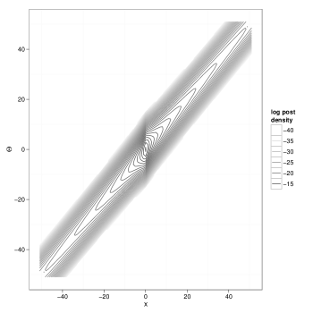
Figure 1: Contours of the ”true” posterior distribution of the non-Gaussian linear model example.

GDS is a more effective alternative for sampling from the posterior distribution. The posterior mode and Hessian of the log posterior at the mode, are $\theta^{*}=(0,0)$ and $H=\left(\begin{array}[]{cc}-2.2&0.2\\ 0.2&-0.2\end{array}\right)$. The GDS proposal distribution $g(\theta)$ is taken to be a bivariate normal with mean $\theta^{*}$ and covariance $-sH^{-1}$, with $s=200$. This scaling factor was the smallest value of $s$ for which $\Phi(\theta)\leq 1$ for all $M=20,000$ of the proposal draws. Two hundred independent samples were collected using the GDS algorithm.

Figure 2 plots each of the GDS draws, where darker areas represent higher values of log posterior density. GDS not only picks up the correct shape of the regions of high posterior mass near the origin, but also the dependence in the long tails. The acceptance rate to collect these draws was about 0.013.

In contrast, consider Figure 3. which plots samples collected using MCMC. Specifically, we used the RH-MALA method in Girolami and Calderhead (2012), with constant curvature, estimating the Hessian at each iteration. These are samples from 25,000 iterations, collected after starting at the posterior mode and running through 25,000 burn-in iterations, thinned every 10 draws. Just as Papaspiliopolous and Roberts predicted, the chain tends to get stuck near the mode. It is only after some serendipitously large proposal jumps that the chain ever finds itself in the tails (hence the gaps in the plot), but the chain does not move very far along those tails at all.

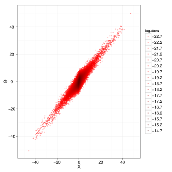
Figure 2: Posterior draws from non-Gaussian linear regression example, using GDS. Darker colors represent regions of higher posterior density

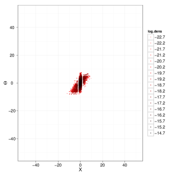
Figure 3: Posterior draws from non-Gaussian linear regression example, using MCMC. Darker colors represent regions of higher posterior density

3.2 Hierarchical Gaussian model

Next, we consider a hierarchical model with a large number of parameters. The dependent variable $y_{it}$ is measured $T$ times for heterogenous units $i=1\mathellipsis n$. For each unit, there are $k$ covariates, including an intercept. The intercept and coefficients $\beta_{i}$ are heterogeneous, with a Gaussian prior with mean $\bar{\beta}$ and covariance $\Omega$, which in turn have weakly information standard hyperpriors. This model structure is given by:

$$y_{it} \sim N(x_{i}^{\prime}\beta_{i},1),~{}i=1\mathellipsis n,~{}t=1\mathellipsis T$$ (15)

$$\beta_{i}|\Omega \sim MVN(\bar{\beta},\Omega)$$ (16)

$$\bar{\beta} \sim MVN(0,V_{\beta})$$ (17)

$$\Omega \sim IW(\nu,A)$$ (18)

To construct simulated datasets, we set “true” values of $\bar{\beta}=(5,0,-2,0)$ and $\Omega=0.25I$. For each unit, we simulated $T=25$ observations, where the non-intercept covariates are all i.i.d draws from a standard normal distribution. Three different values for $n$ were entertained: 100, 500 and 1000. In all cases, there are 14 population-level parameters, so the total number of parameters are 414, 2014 and 4014, respectively. The parameters of the hyperpriors are $\nu=10$, $V_{\beta}=0.2I$, and $A=0.1I$.

Table 1 summarizes the performance of the GDS algorithm, averaged over 10 replications of the experiment. For each case, we collected 100 samples from the posterior, with $M=10,000$ proposal draws. The proposal distributions are all multivariate normal, with mean at the posterior mode and the covariance set as the inverse of the Hessian at the mode, multiplied by a scale factor that changes with $n$. For each value of $n$, we set the scale factor to roughly be the smallest value for which $\Phi(\theta|y)\leq 1$ for all $M=10,000$ proposal draws. The “Mean Proposals” column is the average number of proposals it took to collect 100 posterior draws during the accept-reject phase of the algorithm (this is the inverse of the acceptance rate). We also recorded the time it took to run each stage of the algorithm. The “Post Mode” column is the number of minutes it took to find the posterior mode, starting at the origin (after transforming all parameters to have a domain on the real line). The “Proposals” column is the amount of time it took to collect the $M=10,000$ proposal draws. “Acc-Rej” is the time it took to execute the accept-reject phase of the algorithm to collect 100 independent samples from the posterior, and “Total” is the total time required to run the algorithm. The study was conducted on an Apple Mac Pro with 12 CPU cores running at 2.93GHz and 32GB of RAM. Ten of the 12 cores were allocated to this algorithm.

	Total	scale	Mean	Minutes for GDS stages
$n$	params	factor	Proposals	Post Mode	Proposals	Acc-Rej	Total
100	414	1.32	15489	0.01	0.11	1.9	2.1
500	2014	1.20	23387	0.08	0.18	11.3	11.6
1000	4014	1.14	26480	0.24	0.28	23.0	23.6

Table 1: Efficiency of GDS for hierarchical Gaussian example

Although Mean Proposals may appear to be high, assessing the efficiency of an algorithm by examining the acceptance rate alone can be misleading. For a single estimation chain, MCMC cannot be run in parallel, while for GDS, all draws can be generated in parallel. For example, each of the 10 cores on the CPU was responsible for collecting 10 posterior samples. One possible counterargument would be that MCMC can be run with multiple chains in parallel, as suggested in Gelman and Rubin (1992). However, if one does use parallel chains, all of the chains need to be burned in independently. There is no guarantee that any one of the chains would have converged after some arbitrary number of iterations, and there will still be residual interdependence in the final set of collected draws. It would be more appropriate to compare the total number of proposals from the GDS rejection sampling phase to the number of post-burn-in iterations that MCMC runs require reaching an effective sample size of 100. It is also worth reiterating that GDS is quite simple to implement, as the algorithm requires no ongoing tuning or adaptation once the accept-reject phase begins.

As a point of comparison, we estimated the posterior for the $n=500$ case using the adaptive Metropolis-adjusted Langevin algorithm with truncated drift (Atchade 2006). We chose this algorithm because it is commonly used, not too hard to implement (relative to many other MCMC variants lie Gibbs sampling), generically applicable to a general class of models that are similar to those for which GDS would work well, and exploits the gradient information that GDS uses to find the posterior mode. We started the chain at the posterior mode, and let it run for 5.5 million iterations, during the course of several weeks. Using the Geweke convergence diagnostic criterion on the log posterior density (Geweke 1991), we decided that only the final 180,000 draws could be considered “post burn-in.” However, those draws represented an effective sample size of only 1,460, suggesting a required thinning ratio of about 1 in 12,000. We did try some more advanced algorithms, such as Girolami and Calderhead(2012), but had difficulty when the chain entered regions for which the Hessian was not negative definite. The Atchade algorithm generates updates of the proposal covariance that are guaranteed to be positive definite. Regardless, this case illustrates how unreliable (and unpredictable) MCMC can be for collecting posterior samples quickly and easily.

3.3 An example of a complex, high-dimensional model

In this section, we consider another model for which GDS should be an attractive estimation method: the effectiveness of online advertising campaigns. Using GDS, we estimate the posterior density from the model described in Braun and Moe (2012). This model is quite complicated; for 5,803 anonymous users, they observe which website advertisements (if any) were served to each user during the course of that user’s web browsing activity. They also observe when these users visited the advertiser’s own website (if ever), and if these website visits resulted in a conversion to a sale. The managerial objective is to develop a method for firms to identify which versions of ads are most likely to generate site visits and sales, taking into account the fact that the return on investment of the ad may not occur until several weeks in the future. The model allows each version of an ad to have a contemporaneous effect in that week, but for each repeat view of the same ad to an incrementally smaller effect. The effect of the ad campaign for an individual builds up with each subsequent ad impression, but this accumulated “ad stock” decays from week to week.

All together, there are 29,073 parameters in the model, consisting of five heterogeneous parameters per user, plus 58 population-level parameters. The data are modeled as being generated from zero-inflated Poisson (for ads and visits) and binomial (for successes) distributions, with the rate parameters being correlated, and dependent on a latent ad stock variable. The ad stock, in turn, is depends on which version of the ad is served, along with nonlinear representations of build-up, wear-out and restoration effects. Given the complex hierarchical structure, extensive nonlinearities, and high degree of correlation in the posterior distribution, attempts at MCMC estimation proved to be well-nigh impossible to implement.

GDS, however, worked well. Because the user-level data are conditionally independent, we could write the log posterior density as the sum of user-level data likelihoods, plus the priors and hyperpriors. Algorithmic differentiation software (Bell 2012) automatically computed the gradients and Hessians for the model. This allows us to find the posterior mode, and estimate the Hessian at the mode, relatively quickly. As above, the proposal density was a multivariate normal, centered at the posterior mode, with a covariance matrix of 1.02 times the inverse of the Hessian at the model. Since the model assumes conditional independence across users, the Hessian of the log posterior has a sparse structure. We exploit this sparsity to generate the proposal draws efficiently, and to dramatically reduce the memory footprint of the algorithm.

To collect 100 independent draws, it took 23.75 minutes. The mean attempts per draw is 2350. Although this may appear like a low acceptance rate, consider that we were able to collect the draws in parallel, without any tuning or adaptation of the algorithm beyond the initial choice of the proposal density. Also, because the sparse Hessian has a “block-diagonal-arrow” structure, it grows only linearly with the number of users.

4 Estimating Marginal Likelihoods

Now, we turn to another advantage of GDS: the ability to generate accurate estimates of the marginal likelihood of the data with little additional computation. A number of researchers have proposed methods to approximate the marginal likelihood, $\mathcal{L}(y)$, from MCMC output. Popular examples include Gelfand and Dey (1994), Newton and Raftery (1994), Chib (1995) and Raftery, et. al. (2007). But none of these methods have achieved universal acceptance as being unbiased, stable or easy to compute. In fact, Lenk (2009) demonstrated that methods which depend solely on samples from the posterior density could suffer from a “pseudo-bias,” and he proposes a method to correct for it. Through several examples, he demonstrates that his method dominates other popular methods, although with substantial computational effort. Thus, the estimation of the marginal likelihood of a dataset, and its use in model selection, remains a difficult problem in MCMC-based Bayesian statistics for which there is no satisfactory solution.

To estimate the marginal likelihood from GDS output, we need the acceptance rate from the accept-reject stage of the algorithm. Recall that $q(u)$ is the probability that, given a threshold value $u$, a proposal from $g(\theta)$ is accepted. Therefore, one can express the expected marginal acceptance probability for any posterior draw as

$$\gamma =\int_{0}^{1}q(u)p(u|y)~{}du.$$ (19)

Substituting Equation 6,

$$\gamma =\frac{c_{1}}{c_{2}\mathcal{L}(y)}\int_{0}^{1}q^{2}(u)~{}du$$ (20)

Applying the change of variables so $v=-\log u$, and then rearranging terms,

$$\mathcal{L}(y) =-\frac{c_{1}}{c_{2}\gamma}\int_{0}^{\infty}q^{2}(v)\exp(-v)~{}dv.$$ (21)

The values for $c_{1}$ and $c_{2}$ are immediately available from the GDS algorithm. One can estimate $\gamma$ by treating the number of proposals required to accept a posterior draw as a shifted geometric random variable (an acceptance on the first proposal is a count of 1). Thus, an estimator of $\gamma$ is the inverse of the mean number of proposals per draw.

What remains is estimating the integral in Equation 21. This is done by using the proposal draws from Step 5 in the GDS algorithm in Section 2. The empirical CDF of these draws is discrete, so we can partition the support of $q(v)$ at $v_{1}\mathellipsis v_{M}$. Also, since $q_{M}(v)$ is the proportion of proposal draws less than $v$, we have $q_{M}(v)=\frac{i}{M}$. Therefore,

$$\int_{0}^{\infty}q^{2}(v)\exp(-v)dv \approx\sum_{i=1}^{M}\int_{v_{i}}^{v_{i+1}}\left(\frac{i}{M}\right)^{2}\exp(-v_{i})dv$$ (22)

$$=\frac{1}{M^{2}}\sum_{i=1}^{M}i^{2}\left[\exp(-v_{i})-\exp(-v_{i+1})\right]$$ (23)

$$=\frac{1}{M^{2}}\sum_{i=1}^{M}\left(2i-1\right)\exp(-v_{i})$$ (24)

(By convention, define $v_{M+1}=\infty$). Putting all of this together, we can estimate the marginal likelihood as

$$\mathcal{L}(y) \approx\frac{c_{1}}{M^{2}c_{2}\gamma}\sum_{i=1}^{M}(2i-1)\exp(-v_{i})$$ (25)

As a demonstration of the accuracy of this method, consider the following normal linear regression model, also used by Lenk (2009) to demonstrate the accuracy of his method.

$$y_{it} \sim N(x_{i}^{\prime}\beta,\sigma^{2}),~{}i=1\mathellipsis n,t=1\mathellipsis T$$ (26)

$$\beta|\sigma \sim N(\beta_{0},\sigma^{2}V_{0})$$ (27)

$$\sigma^{2} \sim IG(r,\alpha)$$ (28)

For this model, $\mathcal{L}(y)$ is a multivariate-T density. This allows us to compare the estimates of $\mathcal{L}(y)$ from GDS with “truth.” To do this, we conducted a simulation study for simulated datasets of different sizes ($n$=200 or 2000) and numbers of covariates ($k$=5, 25 or 100). For each $n,k$ pair, we simulated 25 datasets. For each dataset, each vector $x_{i}$ includes an intercept and $k$ iid samples from a standard normal density. There are $k+2$ parameters, corresponding to the elements of $\beta$, plus $\sigma$. The true intercept term is 5, and the remaining true $\beta$ parameters are linearly spaced from $-5$ to $5$. In all cases, there are $T=25$ observations per unit. Hyperpriors are set as $r=2$, $\alpha=1$, $\beta_{0}$ as a zero vector and $V_{0}=0.2\cdot I_{k}$.

For each dataset, we collected 250 draws from the posterior density using GDS, with different numbers of proposal draws ($M$=1,000 or 10,000), and scale factors ($s=$0.5, 0.6, 0.7 or 0.8) on the Hessian (so $sH$ is the precision matrix of the MVN proposal density, and lower scale factors generate more diffuse proposals). The $s=0.8$ and $n=200$ cases were excluded because the proposal density was not sufficiently diffuse that $\Phi(\theta|y)$ was between 0 and 1 for the $M$ proposal draws. Table 2 presents the true log marginal likelihood (MVT), along with estimates using GDS, the importance sampling method in Lenk (2009), and the harmonic mean estimator (Newton and Raftery 1994). Table 3 shows the mean absolute percentage error (MAPE) of the GDS and Lenk methods, relative to the true log likelihood. The acceptance percentages for each dataset, and the time it took to generate 250 posterior draws (after finding the posterior mode) are also summarized.

What we can see from these tables is that the GDS estimates for the log marginal likelihood are remarkably close to the multivariate T densities, and are robust when we use different scale factors. Accuracy appears to be better for larger datasets than smaller ones, and improving the approximation of $p(u)$ by increasing the number of proposal draws offers negligible improvement. Note that the performance of the GDS method is comparable to that of Lenk, but is much better than the harmonic mean estimator. We did not compare our method to others (e.g., Gelfand and Dey 1994), because Lenk already did that when demonstrating the importance of correcting for pseudo-bias, and how his method dominates many other popular ones. The GDS method is similar to Lenk’s in that it computes the probability that a proposal draw falls within the support of the posterior density. However, note that the inputs to the GDS estimator are intrinsically generated as the GDS algorithm progresses, while computing the Lenk estimator requires an additional importance sampling run after the MCMC draws are collected. We are not claiming that our method is better than Lenk’s. Instead, this illustration shows that one of the important advantages of GDS is the ease and accuracy with which one can estimate marginal likelihoods.

				MVT		GDS		Lenk		HME
k	n	M	scale	mean	sd	mean	sd	mean	sd	mean	sd
5	200	1000	0.5	-309	6.6	-309	6.6	-311	6.8	-287	7.1
5	200	1000	0.6	-309	6.6	-309	6.7	-310	6.9	-287	6.9
5	200	1000	0.7	-309	6.6	-309	6.7	-310	6.5	-287	6.3
5	200	10000	0.5	-309	6.6	-309	6.6	-311	6.7	-287	6.7
5	200	10000	0.6	-309	6.6	-309	6.6	-310	7.5	-287	6.8
5	200	10000	0.7	-309	6.6	-309	6.7	-310	7.0	-287	7.1
5	2000	1000	0.5	-2866	46.2	-2865	46.3	-2868	46.2	-2836	46.2
5	2000	1000	0.6	-2866	46.2	-2866	46.2	-2868	45.7	-2836	45.5
5	2000	1000	0.7	-2866	46.2	-2866	46.3	-2867	45.9	-2836	45.9
5	2000	1000	0.8	-2866	46.2	-2866	46.2	-2867	46.3	-2835	46.3
5	2000	10000	0.5	-2866	46.2	-2866	46.4	-2867	46.7	-2836	46.9
5	2000	10000	0.6	-2866	46.2	-2866	46.2	-2867	45.8	-2836	46.3
5	2000	10000	0.7	-2866	46.2	-2866	46.4	-2867	46.0	-2836	46.3
5	2000	10000	0.8	-2866	46.2	-2866	46.2	-2867	46.5	-2835	46.3
25	200	1000	0.5	-387	8.1	-385	8.2	-391	7.6	-292	8.5
25	200	1000	0.6	-387	8.1	-386	8.1	-390	9.5	-292	8.8
25	200	1000	0.7	-387	8.1	-386	8.3	-390	8.0	-292	8.8
25	200	10000	0.5	-387	8.1	-385	8.5	-390	8.2	-292	8.4
25	200	10000	0.6	-387	8.1	-385	8.2	-390	8.9	-292	8.8
25	200	10000	0.7	-387	8.1	-386	8.2	-390	8.7	-292	9.1
25	2000	1000	0.5	-2990	28.7	-2989	28.8	-2994	28.3	-2865	28.8
25	2000	1000	0.6	-2990	28.7	-2989	28.7	-2993	28.4	-2864	29.0
25	2000	1000	0.7	-2990	28.7	-2989	28.9	-2991	30.0	-2864	29.5
25	2000	1000	0.8	-2990	28.7	-2990	28.7	-2992	29.6	-2864	29.4
25	2000	10000	0.5	-2990	28.7	-2988	29.2	-2992	28.5	-2864	28.9
25	2000	10000	0.6	-2990	28.7	-2989	29.1	-2993	29.4	-2864	28.9
25	2000	10000	0.7	-2990	28.7	-2990	29.0	-2993	28.9	-2864	28.9
25	2000	10000	0.8	-2990	28.7	-2990	28.6	-2993	28.2	-2865	28.2
100	200	1000	0.5	-660	6.7	-661	6.5	-683	8.8	-292	9.2
100	200	1000	0.6	-660	6.7	-660	6.6	-678	8.5	-286	9.0
100	200	1000	0.7	-660	6.7	-659	7.1	-673	7.8	-282	8.0
100	200	10000	0.5	-660	6.7	-659	6.9	-682	9.1	-288	10.4
100	200	10000	0.6	-660	6.7	-660	5.7	-678	8.8	-286	8.9
100	200	10000	0.7	-660	6.7	-658	6.7	-674	7.3	-282	8.4
100	2000	1000	0.5	-3364	24.4	-3364	24.8	-3370	27.5	-2871	27.1
100	2000	1000	0.6	-3364	24.4	-3362	24.6	-3369	24.3	-2868	25.3
100	2000	1000	0.7	-3364	24.4	-3361	23.9	-3371	25.6	-2870	25.4
100	2000	1000	0.8	-3364	24.4	-3362	23.9	-3370	26.0	-2868	26.1
100	2000	10000	0.5	-3364	24.4	-3362	24.0	-3372	25.3	-2870	25.2
100	2000	10000	0.6	-3364	24.4	-3360	24.9	-3368	25.3	-2867	25.4
100	2000	10000	0.7	-3364	24.4	-3360	24.6	-3370	25.5	-2869	25.5
100	2000	10000	0.8	-3364	24.4	-3362	24.5	-3367	24.3	-2867	24.4

Table 2: Results of simulation study for effectiveness of estimator for log marginal likelihood.

				MAPE-GDS		MAPE-LENK		Accept %		Time (mins)
k	n	M	scale	mean	sd	mean	sd	mean	sd	mean	sd
5	200	1000	0.5	0.23	0.16	0.47	0.39	22.05	7.64	0.09	0.24
5	200	1000	0.6	0.11	0.12	0.52	0.45	40.46	10.82	0.02	0.04
5	200	1000	0.7	0.06	0.05	0.47	0.39	57.13	8.46	0.01	0.00
5	200	10000	0.5	0.17	0.08	0.50	0.37	23.99	5.32	0.04	0.01
5	200	10000	0.6	0.10	0.06	0.54	0.46	40.85	7.19	0.04	0.01
5	200	10000	0.7	0.07	0.07	0.48	0.35	55.15	9.15	0.04	0.01
5	2000	1000	0.5	0.02	0.01	0.07	0.05	22.14	7.65	0.04	0.07
5	2000	1000	0.6	0.01	0.01	0.06	0.06	37.76	10.34	0.03	0.08
5	2000	1000	0.7	0.01	0.01	0.06	0.05	49.55	13.39	0.01	0.00
5	2000	1000	0.8	0.01	0.01	0.04	0.02	64.60	12.93	0.01	0.00
5	2000	10000	0.5	0.02	0.01	0.05	0.05	25.30	6.65	0.06	0.07
5	2000	10000	0.6	0.01	0.01	0.04	0.03	36.28	7.06	0.04	0.01
5	2000	10000	0.7	0.01	0.01	0.05	0.03	51.43	14.49	0.05	0.03
5	2000	10000	0.8	0.00	0.01	0.04	0.03	71.95	11.83	0.04	0.00
25	200	1000	0.5	0.49	0.36	0.98	0.47	2.77	2.50	0.47	0.60
25	200	1000	0.6	0.26	0.13	1.06	0.46	8.07	3.36	0.13	0.18
25	200	1000	0.7	0.18	0.10	0.80	0.43	16.16	5.08	0.06	0.11
25	200	10000	0.5	0.52	0.25	0.93	0.65	1.67	0.87	1.15	1.99
25	200	10000	0.6	0.35	0.19	1.03	0.68	6.24	3.72	0.72	1.39
25	200	10000	0.7	0.11	0.05	0.88	0.77	20.01	3.23	0.04	0.01
25	2000	1000	0.5	0.04	0.03	0.11	0.10	2.69	1.98	0.28	0.25
25	2000	1000	0.6	0.06	0.03	0.09	0.06	4.57	3.03	0.75	1.02
25	2000	1000	0.7	0.04	0.03	0.09	0.09	15.44	9.61	0.59	1.36
25	2000	1000	0.8	0.01	0.01	0.09	0.07	43.14	12.62	0.03	0.02
25	2000	10000	0.5	0.10	0.05	0.08	0.06	0.75	0.68	4.34	9.53
25	2000	10000	0.6	0.07	0.03	0.09	0.05	3.65	2.76	1.97	5.95
25	2000	10000	0.7	0.03	0.03	0.08	0.06	17.07	6.33	0.42	1.45
25	2000	10000	0.8	0.01	0.01	0.10	0.08	43.27	10.27	0.05	0.01
100	200	1000	0.5	0.27	0.23	3.50	0.82	0.32	0.29	0.49	0.85
100	200	1000	0.6	0.17	0.22	2.74	0.71	0.30	0.22	1.05	3.06
100	200	1000	0.7	0.26	0.22	1.93	0.81	0.40	0.37	1.17	2.18
100	200	10000	0.5	0.20	0.12	3.21	0.93	0.04	0.03	9.64	24.67
100	200	10000	0.6	0.22	0.14	2.62	0.75	0.08	0.07	7.62	27.89
100	200	10000	0.7	0.28	0.17	2.18	0.64	0.08	0.06	1.66	1.62
100	2000	1000	0.5	0.06	0.05	0.24	0.14	0.34	0.38	12.03	26.31
100	2000	1000	0.6	0.04	0.04	0.19	0.12	0.60	0.53	4.61	10.84
100	2000	1000	0.7	0.07	0.04	0.23	0.13	1.10	0.88	3.66	8.46
100	2000	1000	0.8	0.06	0.03	0.21	0.12	3.16	2.26	2.74	8.74
100	2000	10000	0.5	0.05	0.04	0.27	0.12	0.04	0.05	52.26	85.06
100	2000	10000	0.6	0.08	0.05	0.15	0.13	0.14	0.16	64.11	189.53
100	2000	10000	0.7	0.09	0.04	0.19	0.13	0.44	0.42	11.31	23.94
100	2000	10000	0.8	0.05	0.02	0.15	0.11	3.04	1.81	2.08	4.04

Table 3: Results of simulation study for effectiveness of estimator for log marginal likelihood.

5 Practical considerations and limitations of GDS

This section discusses some practical issues while implementing GDS. Like the entire body of MCMC research continues to teach us, more insights will likely be gleaned as we, and hopefully others, gain additional experience with the method. Here, we provide some suggestions on how to implement GDS effectively, and mention some areas in which more research or investigation is needed.

5.1 Finding the posterior mode and estimating the Hessian

Searching for the posterior mode is considered, in general, to be “good practice” for Bayesian inference even when using MCMC; see Step 1 of the “Recommended Strategy for Posterior Simulation” in Section 11.10 of Gelman et. al (2003). For small problems, like the example in Section 3.1, standard nonlinear optimization algorithms, such as those found in common statistical packages like R, are sufficient for finding posterior modes and estimating Hessians. For larger problems, finding the mode and estimating the Hessian can be more difficult when using those same tools. However, there are many different ways to find the extrema of a function, and some may be more appropriate for some kinds of problems than for others. Therefore, one should not immediately conclude that finding the posterior mode (or modes) is a barrier to adopting GDS for large or ill-conditioned problems, like the $29,073$-dimensional model in Section 3.3.

When the log posterior density is smooth and unimodal, a natural algorithm for finding a posterior mode is one that exploits gradient and Hessian information in a way that is related to Newton’s Method. Nocedal and Wright (2006) describe many different nonlinear optimization methods, but most can be classified as either “line search” or “trust region” methods. Line search methods may be more common; for instance, all of the gradient-based algorithms implemented in the optim function in R are line search methods. But these methods could be subject to numerical problems when the log posterior is nearly flat, or has a ridge, in which case the algorithm may try to evaluate the log posterior at a point that is so far away from the current value that it generates numerical overflow. Trust region methods (Conn, et. al., 2000), on the other hand, tend to be more stable, because each proposed step is constrained to be within a particular distance (the “radius” of the trust region) of the current point. In short, if one finds that a “standard” optimizer for a particular programming environment is having trouble finding the posterior mode, there may be other common algorithms that can find the mode more easily.

Neither line-search nor trust-region algorithms necessarily require explicit expressions for gradients and Hessians, but generating these structures exactly can also speed up the mode-finding step of GDS. This approach is in contrast to approximations that use finite differencing or quasi-Newton Hessian updates. Of course, one can always derive the gradient of the log posterior density analytically, but this can be a tedious process. We have had success with algorithmic differentiation (AD) software such as the CppAD library (Bell 2012). With AD, we need only to write a function that computes the log posterior density. The AD library includes functions that automatically return derivatives of that function. The time to compute the gradient of a function is a small multiple of the time it takes to compute the original function, and otherwise does not depend on the dimension of the problem.

Estimating the Hessian is useful not only for the mode-finding step, but also for choosing the covariance matrix of a multivariate proposal density. The time it takes for AD software to compute a Hessian can depend on the dimension of the problem, and working with a dense Hessian for a large problem can be prohibitively expensive in terms of computation and memory usage. However, for many hierarchical models, we assume conditional independence across heterogeneous units. For these models, the Hessian of the log posterior is sparse, with a “block-diagonal-arrow” structure (block-diagonal, but dense on the bottom and right margins). Thus, we can achieve substantial computational improvements by exploiting this sparsity. The advantage comes in storing the Hessian in a compressed format, such that zeros are not stored explicitly. Not only does this permit estimating larger models on computers with less memory, but it also lets us use efficient computational routines that exploit that sparsity. For example, Powell and Toint (1979) and Coleman and More (1983) explain how to efficiently estimate sparse Hessians using graph coloring techniques. Coleman et al. (1985a, 1985b) offer a useful FORTRAN implementation to estimate sparse Hessians using graph coloring and finite differencing. Algorithmic differentiation libraries like CppAD can also exploit sparsity when computing Hessians. Both MATLAB and R (through the Matrix package) can store sparse symmetric matrices in compressed format.

One important consideration is the case of multimodal posteriors. GDS does require finding the global posterior mode, and all the models discussed in this paper have unimodal posterior distributions. When the posterior is multimodal, one could instead use a mixture of normals as the proposal distribution. The idea is to not only find the global mode, but any local ones as well, and center each mixture component at each of those local modes. The GDS algorithm itself remains unchanged, as long as the global posterior mode matches the global proposal mode.

We recognize that finding all of the local modes could be a hard problem, and there is no guarantee that any optimization algorithm will find all local extrema. But, by the same token, this problem can be resolved efficiently in a multitude of complex Bayesian statistical models if one uses the correct tools. And it is only a matter of time before these tools are more widely available in standard statistical programming languages like R. The nonlinear optimization literature is rife with methods that help facilitate efficient location of multiple modes, even if there is no guarantee of finding them all. Also, note that even though MCMC sampling chains are, in theory, guaranteed to explore the entire space of any posterior distribution (including multiple regions of high posterior mass), there is no guarantee that this will happen after a large finite number of iterations for general nonconjugate hierarchical models. Other estimation algorithms that purport to be robust to multimodal posteriors offer no such guarantees either.

5.2 Choosing a proposal distribution

Like many other methods that collect random samples from posterior distributions, the efficiency of GDS depends in part on a prudent selection of the proposal density $g(\theta)$. For the examples in this paper, we used a multivariate normal density that is centered at the posterior mode, with a covariance matrix that is proportional to the inverse of the Hessian at the mode. One might then wonder if there is an optimal way to determine just how “scaled out” the proposal covariance needs to be. At this time, we think that trial and error is, quite frankly, the best alternative. For example, if we start with a small $M$ (say, 100 draws), and find that $\Phi(\theta|y)>1$ for any of the $M$ proposals, we have learned that the proposal density is not valid, at little computational or real-time cost. We can then re-scale the proposal until $\Phi(\theta|y)<1$, and then gradually increase $M$ until we get a good approximation to $p(u)$. In our experience, even if an acceptance rate appears to be low (say, 0.0001), we can still collect draws in parallel, so the “clock time” remains much less than the time we spend trying to optimize selection of the proposal.

For example, in the Cauchy example in Section 3.1, we set the proposal covariance to be the inverse Hessian at the posterior mode, scaled by a factor of 200. We needed such a large scale factor because the normal approximation at the mode shows no correlation, even though there is obvious correlation in the tails. If one knew upfront the extent of the tail dependence, one might have chosen a proposal density that is more highly correlated, and that might give a higher acceptance rate. But of course one seldom, if ever, knows the shape of any target posterior density up front. So even though an acceptance percentage of 1.3% may appear to be low, we should consider the amount of time it would take to improve the proposal density, and especially the number of MCMC iterations it would take to get enough draws that are equivalent to the same number of independent GDS draws.

5.3 Cases requiring further research

This paper demonstrated that GDS is a viable alternative to MCMC for a large class of Bayesian non-Gaussian and Gaussian hierarchical models. Of course it would be myopic to claim that GDS is appropriate for all models. By the same token, we cannot assert that GDS would not work for any of the models described below. These models are topics requiring additional research.

Models with discrete or combinatorial optimization elements

In models that include both discrete and continuous parameters, finding the posterior mode becomes a mixed-integer nonlinear program (MINLP). An example is the Bayesian variable selection problem (George and McCulloch 1997). The difficulty lies in the fact that MINLPs are known to be NP-complete, and thus may not scale well for large problems. Hidden Markov models with multiple discrete states might be similarly difficult to estimate using GDS. Also, it is not immediately clear how one might select a proposal density when some parameters are discrete.

Intractable likelihoods or posteriors

There are many popular models, namely binary, ordered and multinomial probit models, for which the likelihood of the observed data is not available in closed form. When direct numerical approximations to these likelihoods (e.g., Monte Carlo integration) is not tractable, MCMC with data augmentation is a popular estimation tool (e.g., Albert and Chib 1993). That said, recent advances in parallelization using graphical processing units (GPUs) might make numerical estimation of integrals more practical than it was even 10 years ago; see Suchard et al. (2010). If this is the case, and the log posterior remains sufficiently smooth, then GDS could be a viable, efficient alternative to data augmentation in these kinds of models.

Missing data problems

MCMC-based approaches to multiple imputation of missing data could suffer from the same kinds of problems: the latent parameter, introduced for the data augmentation step, is only weakly identified on its own. Normally, we are not interested in the missing values themselves. If the number of missing data points is small, perhaps one could treat the representation of the missing data points as if they were parameters. But the implications of this require additional research.

Spatial models, and other models with dense Hessians

GDS does not explicitly require conditional independence, so one might consider using it for spatial or contagion models (e.g., Yang and Allenby 2003). However, without a conditional independence assumption, the Hessian of the log posterior will not be sparse, and that may restrict the size of datasets for which GDS is practical.

6 Conclusions

In this paper, we presented a new method, Generalized Direct Sampling (GDS), to sample from posterior distributions. This method has the potential to bypass MCMC-based Bayesian inference for large, complex models with continuous, bounded posterior densities. Unlike MCMC, GDS generates independent draws that one could collect in parallel. The implementation of GDS is straightforward, and requires only a function that returns the value of the unnormalized log posterior density. In addition, GDS allows for fast and accurate computation of marginal likelihoods, which can then be used for model comparison.

There are many other ways to conduct Bayesian inference, and continued improvement of MCMC remains an important stream of research. Nevertheless, it would be hard to ignore the opportunities for parallelization that make algorithms like GDS very attractive alternatives. Of course, one could employ parallel computational techniques as part of a sequential algorithm. But, to repeat an earlier sentence, using parallel technology to generate a single draw is not the same as generating all of the required draws themselves in parallel. By exploiting the advantages of parallel computing, as in this paper, GDS could prove to be a successful addition to the Bayesian practitioner’s computational toolkit.

References

- [1] Atchade, Y. F. (2006) An Adaptive Version for the Metropolis Adjusted Langevin Algorithm with a Truncated Drift. Methodology and Computing in Applied Probability 8, 235-254.
- [2] Bell, B. (2012) CppAD: A Package for C++ Algorithmic Differentiation. Computational Infrastructure for Operations Research http://www.coin-or.org/CppAD.
- [3] Braun, M. and Moe, W. (2012) Online Advertising Response Models: Incorporating Multiple Creatives and Impression Histories. Working paper. Massachusetts Institute of Technology.
- [4] Coleman, T. F., Garbow, B. S. and Moré, J. J. (1985a) Software for Estimating Sparse Hessian Matrices. ACM Transactions on Mathematical Software 11(4) 363-377.
- [5] Coleman, T. F., Garbow, B. S. and Moré, J. J. (1985b) Algorithm 636: FORTRAN Subroutines for Estimating Sparse Hessian Matrices. ACM Transactions on Mathematical Software 11(4) 378.
- [6] Conn, A., Gould, N., and Toint, P. (2000) Trust-Region Methods Philadelphia: Society for Industrial and Applied Mathematics and Mathematical Programming Society.
- [7] Gelman, A., Carlin, J. B., Stern, H. S., and Rubin, D. B. (2003) Bayesian Data Analysis. Boca Raton, Fla.: Chapman and Hall.
- [8] George, E. I. and McCulloch, R. E. (1997) Approaches for Bayesian Variable Selection. Statistica Sinica 7, 339-373.
- [9] Geweke, J. (1991) Evaluating the Accuracy of Sampling-Based Approaches to the Calculation of Posterior Moments. Bayesian Statistics New York: Oxford University Press. 169-193
- [10] Girolami, M., and Calderhead, B. (2011) Riemann Manifold Langevin and Hamiltonian Monte Carlo. Journal of the Royal Statistical Society, Series B (with discussion), 73, 1-37.
- [11] Lenk, P. (2009) Simulation Pseudo-Bias Correction to the Harmonic Mean Estimator of Integrated Likelihoods. Journal of Computational and Graphical Statistics, 18(4) 941-960.
- [12] Nocedal, J. and Wright, S. J. (2006) Numerical Optimization New York: Springer.
- [13] Papaspiliopoulous, O. and Roberts, G. (2008). Stability of the Gibbs Sampler for Bayesian Hierarchical Models. Annals of Statistics, 36, 95-117.
- [14] Powell, M. J. D. and Toint, Ph. L. (1979) On the Estimation of Sparse Hessian Matrices. SIAM Journal on Numerical Analysis 16(6) 1060-1074.
- [15] Tibbits, M.M., Haran, M. and Liechty, J.C. (2010). Parallel Multivariate Slice Sampling. Statistics and Computing, 21(3), 415-430.
- [16] Walker, S.G., Laud, P.W., Zantedeschi, D., and Damien, P. (2010). Direct Sampling. Journal of Computational and Graphical Statistics, 20(3), 692-713.
- [17] Suchard, M.A., Wang, Q., Chan, C., Frelinger, J., Cron, A., and West, M. (2010). Understanding GPU Programming for Statistical Computation: Studies in Massively Parallel Massive Mixtures. Journal of Computational and Graphical Statistics, 19(2), 419-438.
- [18] Yang, S., and Allenby, G. (2003) Modeling Interdependent Consumer Preferences. Journal of Marketing Research 40(3), 282-294.