A survey on independence-based Markov networks learning

Abstract

The problem of learning the Markov network structure from data has become increasingly important in machine learning, and in many other application fields. Markov networks are probabilistic graphical models, a widely used formalism for handling probability distributions in intelligent systems. This document focuses on a technology called independence-based learning, which allows for the learning of the independence structure of Markov networks from data in an efficient and sound manner, whenever the dataset is sufficiently large, and data is a representative sample of the target distribution. In the analysis of such technology, this work surveys the current state-of-the-art algorithms, discussing its limitations, and posing a series of open problems where future work may produce some advances in the area, in terms of quality and efficiency.

1 Motivation

Nowadays intelligent systems have to reason in realistic domains, storing knowledge of the world, and supporting efficient inference, even when exceptions occur. This is referred to in the literature as reasoning under uncertainty. A popular approach taken for reasoning under uncertainty is the use of probabilistic models, a statistical analysis tool for statistical inference. The statistical inference process is used for drawing conclusions from data by calculating the probability of propositional sentences. An example of a probabilistic model is the tabular probabilistic model, a function represented as a table that assigns a probability to every possible complete assignment in a domain, so that the sum of the probabilities adds up to 1. Figure 1 illustrates an abstract tabular model for a domain with $n$ binary variables $\mathbf{V}=\{X_{0},...,X_{n-1}\}$, consisting on $2^{n}$ tuples, one per possible configuration of variables.

$X_{0}$	$X_{1}$	…	$X_{n-1}$		$\Pr(X_{0},..,X_{n-1})$
0	0	…	0		0.121
0	0	…	1		0.076
.	.	…	.		.
.	.	…	.		.
.	.	…	.		.
1	1	…	0		0.21
1	1	…	1		0.12

Figure 1: An example tabular model over $n$ binary random variables, with $2^{n}$ numerical parameters.

However, the tabular model presents computational and semantic limitations. First, its storage requirements are exponential in the number of variables, and the size of its respective domains. When domains of variables are continuous, such tables are infinite, and in practice some mathematical functions can be used. Nonetheless, in this work the attention is restricted only to discrete distributions, so continuous variables may be considered as discrete variables. Second, queries of interest usually do not involve all the variables, and the cost of computing marginal and conditional probabilities would result in exponential summations of variable combinations. Third, such representation has no clear semantics for humans. The common pattern of human knowledge has probabilistic judgments for a small number of propositions. Therefore, conditional independences are a natural way of representing probability distributions. It is common for people to judge a three-place relationship of conditional dependency, i.e., $X$ influences $Y$, given $Z$.

Using independences may reduce the exponential requirements of the tabular model. For example, making the simple assumption that all the $n$ variables in Figure 1 are mutually independent allows decomposing the joint probability distribution as

$$\Pr(X_{0},...,X_{n-1})=\prod\limits^{n-1}_{i=0}{\Pr(X_{i})}.$$

Such decomposition requires a polynomial number ($n$) of exponentially smaller tables with only two rows. Figure 2 illustrates a model assuming that all the binary variables are mutually independent, consisting only of $n$ tables with $2$ tuples each.

$X_{0}$ $\Pr(X_{0})$ 0 0.21 1 0.79    ,    $X_{1}$ $\Pr(X_{1})$ 0 0.45 1 0.55    …    $X_{n-1}$ $\Pr(X_{n-1})$ 0 0.42 1 0.58

Figure 2: An example model assuming that all the variables of the domain are mutually independent, with $n$ tables of only $2$ numerical parameters each.

To address all these problems, namely the exponential storage requirements, the exponential cost of computing marginal and conditional probabilities, and the lack of explicitness of the model, several researchers in the late 80’s created probabilistic graphical models, or simply, graphical models, a well-established formalism for representing compactly joint probability distributions. They are composed of an independence structure, and a set of numerical parameters. The structure encodes the independences present in the distribution, and then defines a family of probability distributions. The set of numerical parameters defines a unique distribution among this family and quantifies the relationships in the structure. Such representation is explained in more detail in Section 2.

The most important types of graphical models are Bayesian networks and Markov networks Pearl (1988). The well-known Bayesian networks are graphical models for encoding distributions where dependencies are representable by a directed acyclic graph. Markov networks (also known as Markov Random Fields, undirected graphical models, or simply undirected models) encode distributions where dependencies are representable by an undirected graph. Three of the most influential textbooks on this topic published in the last three decades are Pearl (1988), Lauritzen (1996) and Koller and Friedman (2009).

There have been many applications of graphical models in a wide range of fields during recent years. Some examples are present in the areas of computer vision and image analysis. Besag et al (1991) gives two examples, one in archeology, the other in epidemiology; in Anguelov et al (2005), addressing the problem of segmenting 3D scan data into objects or object classes; or Li (2001), a complete textbook that presents an exposition of Markov Random fields to image restoration and edge detection in the low-level domain, and object matching and recognition in the high-level domain. More examples are present in the area of spatial data mining and geostatistics, as those presented in the textbook of  Cressie (1992), where Markov Random Fields are emphasized for modeling spatial lattice data; or more recently, the work of  Shekhar et al (2004) that presents spatial analysis methods and applications for Markov Random Fields in a wide range of fields, including biology, spatial economics, environmental and earth science, ecology, geography, epidemiology, agronomy, forestry and mineral prospection. There are also examples for disease diagnosis, such as Schmidt et al (2008) that presents a Markov Random Fields based method for detecting coronary heart disease processing ultrasound images of echocardiograms. Also in the area of computational biology, Friedman et al (2000) proposes the use of Bayesian networks for discovering interactions among genes. More applications of graphical models are present for evolutive optimization searching, as Larrañaga and Lozano (2002) that describes the use of Bayesian networks for modeling the probability distribution of individuals with high fitness in evolutive algorithms, or more recently, Alden (2007) and Shakya and Santana (2008) proposing Markov networks for the same purpose. Further examples are shown for Information Retrieval by Metzler and Croft (2005) and Cai et al (2007), to model term dependencies using Markov Random Fields; and for malware propagation, Karyotis (2010) analyzes the spatial and contextual dependencies of malware propagation, also using Markov Random Fields. There are many other interesting examples that could be included in this list. Table 1 summarizes all these examples in order to help the readers to choose which method can be a better solution for a certain application.

Table 1: Some example Probabilistic Graphical Models applications.

Application	Reference
• Computer vision, and image analysis, with examples in archeology and epidemiology	Besag et al (1991)
• Segmentition of 3D scan data into objects	Anguelov et al (2005)
• Markov Random Fields for image restoration, edge detection and object matching	Li (2001)
• Markov Random Fields for spatial data minging and geostatistics	Cressie (1992)
• Markov Random Fields for spatial spatial analysis methods in biology, spatial economics, environmental and earth science, ecology, geography, epidemiology, agronomy, forestry and mineral prospection.	Shekhar et al (2004)
• Markov Random Fields method for detecting coronary heart disease.	Schmidt et al (2008)
• Computational biology. Learning of Bayesian networks for discovering interactions among genes.	Friedman et al (2000)
• Bayesian networks for evolutive optimization search.	Larrañaga and Lozano (2002)
• Markov networks for evolutive optimization search.	Alden (2007); Shakya and Santana (2008)
• Information Retrieval. Markov Random Fields for modeling terms dependency.	Metzler and Croft (2005); Cai et al (2007)
• Malware propagation. Markov Random Fields for modeling spatial and contextual dependencies.	Karyotis (2010)

The framework provided by probabilistic graphical models supports three critical capabilities of intelligent systems, as highlighted in the textbook of Koller and Friedman (2009):

• Representation: a compact and declarative model of the knowledge based on graphs. On the one hand, such models are compact, providing a representation of conditional independences present in a probability distribution which is efficient and computationally tractable. The compact representation of graphical models is achieved by exploiting a principle property present in many distributions: variables tend to interact directly with very few others. On the other hand, since the models are graphical, they are declarative, and a human expert can understand and evaluate their semantics and properties.

• Inference: given a graphical model, the most fundamental and yet highly non-trivial task is to compute marginal distributions of one or a few variables. This task is usually called inference. Through marginalization it is possible to compute conditionals and posteriors, and to make predictions. Inference is also a sub-routine of learning tasks, and is therefore the most elementary sub-routine of graphical models. However, as proven by Cooper (1990), exact inference is NP-hard in general. There are several methods for working directly with the structure of graphical models, that are in practice orders of magnitude faster than manipulating explicitly the joint probability distribution. The textbook of Koller and Friedman (2009) provides an extensive discussion on this topic, and describes the most popular methods used, such as variable elimination, Monte Carlo methods, and loopy belief propagation. Other recent works are tree-reweighted message-passing of Wainwright et al (2003), Power EP of Minka (2004), generalized belief propagation of Yedidia et al (2004), and Variational message-passing of Winn and Bishop (2005). A free and open source library, providing implementations of various exact and approximate inference methods for graphical models, was published recently by Mooij (2010).

• Learning: constructing graphical models can be done either by a human expert or by learning it automatically from data. There are many algorithms that model the probability distribution of historical data, returning a graphical model as the solution. They are really useful, since experts knowledge is not always enough to design a proper model. Therefore, some authors consider these algorithms a tool for knowledge discovery. Moreover, when constructing models for a specific problem, it is possible to use the data-driven approach, using some part of the model provided by an expert and filling the details automatically, by fitting the model to data. The large number of success stories claimed using this approach in recent years has resulted in some authors, such as Koller and Friedman, claiming that models produced by this process are usually much better than those purely hand constructed.

In this work, the specific problem of learning the independence structure of Markov networks is reviewed. This is an interesting problem that has resulted in important contributions to this domain in recent years, although many of its core challenges remain unresolved and are under intense deliberation. This work focuses on a technology called independence-based learning, which allows one to infer the independence structure of Markov networks from data in an efficient and sound manner, whenever data is sufficient and a representative sample of the target distribution. An analysis of the current state-of-the-art algorithms for learning Markov networks structure using such technology is presented, discussing its current limitations, and its potential for improving the quality and the efficiency of current approaches.

The rest of the document is structured as follows: Section 2 presents an overview of Markov networks representation. Section 3 discusses the problem of learning Markov networks from data. Section 4 provides a review of current independence-based Markov network structure learning algorithms. Finally, Section 5 analyzes the surveyed independence-based algorithms and discusses their relative advantage as well as disadvantages, concluding with a series of open problems that remain in the domain of independence-based structure learning for Markov networks.

2 Markov networks representation

This section provides an overview of the representation of a specific type of graphical models: Markov networks. Graphical models in general consist of a qualitative and a quantitative component for representing a probability distribution $P$. Such distribution is given over a domain of $n$ variables, denoted $\mathbf{V}=\{X_{0},...,X_{n-1}\}$. The qualitative component is the independence structure $G$ (also known as the network, or the graph) of the model, that represents conditional independences among the domain variables, and then defines a family of probability distributions. The quantitative component is a set of numerical parameters $\boldsymbol{\theta}$, that defines a unique distribution among this family and quantifies the relationships in the structure.

2.1 The independence structure

The independence structure is a compact representation of conditional independences present in the underlying distribution $P$. Two variables $X$ and $Y$ are independent conditioned in a set of variables $\mathbf{Z}$ when knowing the value of $Y$ tells me nothing new about $X$, if I already know the values of variables in $\mathbf{Z}$. In this work, conditional independence is denoted as $(\mathbf{X}\mbox{$\perp\!\!\!\perp$}\mathbf{Y}|\mathbf{Z})$, and $(\mathbf{X}\mbox{$\,\not\!\perp\!\!\!\perp$}\mathbf{Y}|\mathbf{Z})$ denotes conditional dependence.

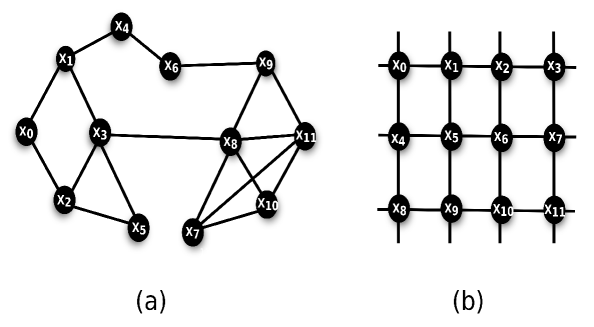
Figure 3: Two examples of undirected independence structure: (a) an irregular graph with different grade of connectivity for distinct nodes, and (b) a regular lattice where variables belong to a domain in a spatial problem.

The structure $G$ of a Markov network is an undirected graph with $n$ nodes, each one representing a random variable in the domain. The edges in the graph encode conditional independences among the variables. Figure 3 shows two examples of undirected structures, both representing domains with $n=12$, and variables $\mathbf{V}=\{X_{0},\dots,X_{11}\}$. The first example in Figure 3 (a) is an irregular graph with different grade of connectivity for distinct nodes. The second in Figure 3 (b) is a regular lattice where variables belong to a domain in a spatial problem, as typically used for representing 2D images, or for two dimensional Ising spin glasses models (mathematical models of ferromagnetism in statistical mechanics).

The independence structure is a map of the independences in the underlying distribution, and such independences can be read from the graph through vertex separation, considering that each variable is conditionally independent of all its non-neighbor variables in the graph, given the set of its neighbor variables. This is called the Local Markov property. For example, in Figure 3 (a) variables $X_{0}$ and $X_{3}$ are conditionally independent, given the set of variables $\{X_{1},X_{2}\}$. In the toroidal lattice of Figure 3 (b), $X_{5}$ is conditionally independent of all the non-adjacent variables, given its neighbor variables $\{X_{1},X_{4},X_{6},X_{9}\}$.

2.1.1 Correctness of the structure

For correctly representing a probability distribution $P$ by a Markov network, $G$ must be a map of the independences present in $P$. As proved in Pearl (1988), a graph $G$ is called an independence-map (or I-map, for short) of a distribution $P$ when all the independences encoded in the graph exist in the underlying distribution $P$.

Definition 1

I-map Pearl (1988)[p.92].

A graph $G$ is an I-map of a distribution $P$ if for all disjoint subsets of variables $\mathbf{X}$, $\mathbf{Y}$ and $\mathbf{Z}$, the following is satisfied:

$${(\mathbf{X}\mbox{$\perp\!\!\!\perp$}\mathbf{Y}|\mathbf{Z})}_{G}\Rightarrow{\langle{\mathbf{X}},{\mathbf{Y}},\mathbf{Z}\rangle}_{P},$$ (1)

where ${(\mathbf{X}\mbox{$\perp\!\!\!\perp$}\mathbf{Y}|\mathbf{Z})}_{G}$ are the independences encoded by $G$, and ${\langle{\mathbf{X}},{\mathbf{Y}},\mathbf{Z}\rangle}_{P}$ are the independences existent in the underlying distribution $P$.

Similarly, $G$ is a dependency-map (D-map) when

$${(\mathbf{X}\mbox{$\perp\!\!\!\perp$}\mathbf{Y}|\mathbf{Z})}_{G}\Leftarrow{\langle{\mathbf{X}},{\mathbf{Y}},\mathbf{Z}\rangle}_{P}.$$ (2)

Using a graph $G$ that is an I-map guarantees that nodes found to be separated correspond to independent variables, but does not guarantee that all those showed to be connected are dependent. Conversely, when $G$ is a D-map it is guaranteed that the nodes connected in $G$ are dependent in the distribution $P$. Fully-connected graphs are trivial I-maps, and empty graphs are trivial D-maps. A distribution $P$ is said to be a perfect-map of $P$ if it is both an I-map and a D-map.

An axiomatic characterization of the family of relations that are isomorphic to vertex separation in graphs is given by the concept of graph-isomorphism. Basically, a distribution $P$ is a graph-isomorph when its independences among variables can be encoded by an undirected graph.

Definition 2

Graph-isomorphism Pearl (1988)[p.93].

A distribution is said to be a graph-isomorph if there exists an undirected graph $G$ that is a perfect-map of $P$, i.e., for every three disjoint subsets $\mathbf{X}$, $\mathbf{Y}$ and $\mathbf{Z}$, we have

$${(\mathbf{X}\mbox{$\perp\!\!\!\perp$}\mathbf{Y}|\mathbf{Z})}_{G}\Longleftrightarrow{\langle{\mathbf{X}},{\mathbf{Y}},\mathbf{Z}\rangle}_{P}.$$ (3)

A necessary and sufficient condition for a distribution $P$ to be a graph-isomorph is that ${\langle{\mathbf{X}},{\mathbf{Y}},\mathbf{Z}\rangle}_{P}$ satisfies the following axioms of independences, introduced by Pearl and Paz (1985). There is another set of axioms for learning Bayesian networks, but it is omitted here.

Symmetry	$(\mathbf{X}\mbox{$\perp\!\!\!\perp$}\mathbf{Y}|\mathbf{Z})\Leftrightarrow(\mathbf{Y}\mbox{$\perp\!\!\!\perp$}\mathbf{X}|\mathbf{Z})$
Decomposition	$(\mathbf{X}\mbox{$\perp\!\!\!\perp$}\mathbf{Y}~{}\cup~{}\mathbf{W}|\mathbf{Z})\Rightarrow(\mathbf{X}\mbox{$\perp\!\!\!\perp$}\mathbf{Y}|\mathbf{Z})~{}\&~{}(\mathbf{X}\mbox{$\perp\!\!\!\perp$}\mathbf{W}|\mathbf{Z})$
Transitivity	$(\mathbf{X}\mbox{$\perp\!\!\!\perp$}\mathbf{Y}|\mathbf{Z})\Rightarrow(\mathbf{X}\mbox{$\perp\!\!\!\perp$}\lambda|\mathbf{Z})~{}\mbox{or}~{}(\lambda\mbox{$\perp\!\!\!\perp$}\mathbf{Y}|\mathbf{Z})$	(4)
Strong union	$(\mathbf{X}\mbox{$\perp\!\!\!\perp$}\mathbf{Y}|\mathbf{Z})\Rightarrow(\mathbf{X}\mbox{$\perp\!\!\!\perp$}\mathbf{Y}|\mathbf{Z}\cup\mathbf{W})$
Intersection	$(\mathbf{X}\mbox{$\perp\!\!\!\perp$}\mathbf{Y}|\mathbf{Z}~{}\cup~{}\mathbf{W})~{}\&~{}(\mathbf{X}\mbox{$\perp\!\!\!\perp$}\mathbf{W}|\mathbf{Z}~{}\cup~{}\mathbf{Y})\Rightarrow(\mathbf{X}\mbox{$\perp\!\!\!\perp$}\mathbf{Y}~{}\cup~{}\mathbf{W}|\mathbf{Z})$,

where $\mathbf{X}$, $\mathbf{Y}$, $\mathbf{Z}$ and $\mathbf{W}$ are all disjoint subsets of the set of all the variables in the domain $\mathbf{V}$, and $\lambda$ stands for a single variable, not in $\mathbf{X}\cup\mathbf{Y}\cup\mathbf{Z}\cup\mathbf{W}$. The intersection axiom is valid only for strictly positive probability distributions. This list of axioms represents the relationships that hold among the independences encoded by the graph.

In summary, when the distribution $P$ is a graph-isomorph, there exists a graph $G$ that is a perfect-map for $P$. For representing a distribution $P$, any graph $G$ which is an I-map of $P$ may be used. However, the more independences of the underlying distribution encoded in the graph, the better the model is in complexity and accuracy when used for inference. Assuming graph-isomorphism is an important decision, since not all the existent distributions may be represented by an undirected graph. For example, there are distributions that may be represented by an acyclic directed graph, and in this case, Bayesian networks are the correct model to use. There are also other distributions that cannot be encoded by a graph.

2.1.2 The Markov blanket concept

This section describes the concept of Markov blanket, a central theoretical concept in the representation of distributions, introduced by Pearl (1988). The Markov blanket of a variable is the only knowledge needed to predict the behavior of that variable. Hence, this concept holds relevance for a wide variety of applications where local relationships to some variables are significant.

Definition 3

The Markov blanket concept.

The Markov blanket of a variable $X$ is a minimal set, denoted here $\mathbf{MB}^{X}$, conditioned on which all other nodes in the domain of variables $\mathbf{V}$ are independent of $X$, that is,

$$\forall Y\in\mathbf{V}-\{\mathbf{MB}^{X}\},~{}(X\mbox{$\perp\!\!\!\perp$}Y|\mathbf{MB}^{X}).$$ (5)

That is, the Markov blanket of a variable is the smallest set of variables that shields it from the probabilistic influence of the variables not in the blanket. From a graphical view point, the Markov blanket of a variable $X$ is identical to its neighbors in the graph.

In the textbook of Pearl (1988), it is proved formally that, for strictly positive distributions, the independence structure can be constructed by piecing together the Markov blanket of all the variables of the domain, connecting with an edge every two variables $X$ and $Y$, such that $X$ belongs to the Markov blanket of $Y$. There is also a proof stating that every variable $X\in\mathbf{V}$ in a distribution that is a graph isomorph, and therefore satisfies the Pearl’s axioms, has a unique Markov blanket. As only strictly positive distributions satisfy the Intersection axiom, this mechanism for constructing the structure only holds for positive distributions.

2.2 Parameterization

This section explains how to quantify the relationships encoded in $G$. Although this work only addresses the problem of structure learning, the quantitative aspects of Markov networks are briefly explained for better clarifying our work. Below is described a factorization method for constructing the Gibbs distribution for an arbitrary undirected graph $G$, provided in Pearl (1988):

• Identification of the maximal subgraphs whose nodes are all adjacent to each other, called the maximal cliques of $G$. For example, the graph in Figure 3 (a) shows a maximal clique of size $4$ among the nodes corresponding to variables $\{7,8,10,11\}$, two maximal cliques of size $3$ among nodes $\{2,3,5\}$ and $\{8,9,11\}$, and the rest of edges are maximal cliques of size $2$. In Figure 3 (b) the size of all the cliques is $2$.

• For each clique $\mathbf{c}\in\mathcal{C}$ in the set of all the cliques in the graph, assign a non-negative potential function $g_{\mathbf{c}}(\mathbf{X}_{\mathbf{c}})$ (where $\mathbf{X}_{\mathbf{c}}$ is the set of variables that belong to the clique $\mathbf{c}$) measuring the relative degree of compatibility associated with each possible configuration of $\mathbf{X}_{\mathbf{c}}$. Usually each potential function is represented by a table with a numerical parameter assigned to each possible complete assignment of the variables that compose the clique, like the tabular model showed in Figure 1, but including only the variables that compose the clique $\mathbf{c}$. A difference with the tabular model is that here the parameter values are not normalized.

• Form the product $\prod\limits_{\mathbf{c}\in\mathcal{C}}{g_{\mathbf{c}}(\mathbf{X}_{\mathbf{c}})}$ of the potential functions over all the cliques.

• Construct the Gibbs distribution by normalizing the product over all possible value combinations of the variables in the system

  $$P(X_{0},..,X_{n-1})=\frac{1}{Z}\prod\limits_{\mathbf{c}\in\mathcal{C}}{g_{\mathbf{c}}(\mathbf{X}_{\mathbf{c}})},$$ (6)

  where Z is the partition function, or normalization constant, computed as

  $$Z=\sum\limits_{X_{0},..,X_{n-1}}{\prod\limits_{\mathbf{c}\in\mathcal{C}}{g_{\mathbf{c}}(\mathbf{X}_{\mathbf{c}})}}.$$ (7)

Using the Hammersley-Clifford theorem it is possible to prove that the general form of the Gibbs distribution of Equation (6) embodies all the conditional independences encoded in the graph $G$. Such form of the Gibbs distribution presents some difficulties. First, it is difficult to discern the meaning of the potential functions. Second, the computational cost of calculating the partition function $Z$ is exponential, as it requires an exponential sum over all possible assignments of the complete set of variables.

3 The Markov networks learning problem

This section discusses the difficulties that arise in the task of learning Markov networks from historical information. This task is only possible whenever the size of the input dataset $D$ is sufficient, and the data is a representative sample of the underlying distribution $P$. When these conditions are satisfied, it is possible that some algorithms learn a model for representing $P$ by exploring and analyzing $D$. The input dataset $D$ contains historical information commonly structured in the tabular format, a standard format in machine learning. This is a file that contains a table with a column per random variable in $P$, and the rows are the datapoints, each one being a complete assignment for all the variables. For example, a datapoint for a domain with $n=4$ random binary variables $\mathbf{V}=\{X_{0},X_{1},X_{2},X_{3}\}$ may be $(X_{0}=0,X_{1}=1,X_{2}=1,X_{3}=0)$. The algorithms discussed in this work ignore the problem of missing values, which is solved by known, yet computationally challenging, statistical techniques.

Learning a Markov network from data is a problem that consists in learning both the structure $G$ and the parameters $\boldsymbol{\theta}$. Of course, the best possible structure learned is a perfect-map, that is, a model that contains a structure encoding all the dependences and the independences present in $P$. However, every model containing a structure which is an I-map of $P$ is a good solution. The closer to a perfect-map, the better is the structure learned, and the better is the resulting Markov network for representing $P$. When learning a model for large domains, a desirable property of the model is the sparsity, since densely connected models require too many parameters, and make exact and even approximate inferences computationally intractable.

3.1 Goals of Markov networks learning

For evaluating the merits of a model learning method, it is important to consider the goal of learning. Clearly, learning the complete model (structure plus parameters) is the ideal method, but due to computational, spatial or sampling limitations, it may not be possible in practice. For that reason, other less ambitious goals are often considered in practice, such as the three main goals of learning discussed by Koller and Friedman (2009):

• Density estimation: A common reason for learning a Markov network is to use it for some inference task. When formulating the goal of learning as one of density estimation, the goal is to construct a model $M$ so that the defined distribution is “close” to the underlying distribution $P$. A common metric for evaluating the quality of such approximation is the use of the likelihood of the data $Pr(D\mid M)$. However, this goal assumes that the overall distribution $P$ is needed.

• Specific prediction tasks: The goal is predicting the distribution of a particular set of variables $\mathbf{Y}$, given certain set of variables $\mathbf{X}$. When the model is used only to perform a particular task, if the model is never evaluated on predictions of the variables $\mathbf{X}$, it is better to optimize the learning task for improving the quality of its answers to $\mathbf{Y}$. This has been the goal of a large fraction of the work in machine learning. For example, consider the problem of documents classification for a given set of relevant words of a document, and a variable that labels the topic of the document. Another well-known example is the task of image segmentation, where the goal of the task is the prediction of class labels for all the pixels in the image, given the image features.

• Knowledge discovery: The goal of knowledge discovery is to learn the correct structure of the underlying distribution. There are some cases when the learned structure can reveal some important unknown properties of the domain. It is a very different motivation for learning the distribution. An examination of the learned structure can show dependences among variables as positive or negative correlations. In a knowledge discovery application, it is far more critical to assess the confidence in a prediction, taking into account the extent to which it can be identified given the available data, and the number of hypotheses that would cause similar observed behavior. For example, in a medical diagnosis domain, we may want to learn the structure of the model to discover which predisposing factors lead to certain diseases, and which symptoms are associated with different diseases.

3.2 Parameters estimation

Markov network parameters estimation is usually used to choose the value of the parameters by fitting the model to data, because tuning parameters manually is often difficult, and learned models often exhibit better performance. This task has shown to be an NP-hard problem by Barahona (1982).

For estimating the parameters, the most common method proposed is maximum-likelihood estimation, potentially using some regularization as an additional parameter prior. Unfortunately, evaluating the likelihood of a complete model requires, for every set of parameters proposed during the maximum-likelihood estimation process, the computation of the partition function $Z$, which is used for normalizing the product over all possible value combinations of the variables of the domain, as showed in Equation (7). Although it is not possible to optimize the maximum-likelihood in a closed form, it is guaranteed that the global optimum can be found, because it is a concave function. As a result, some approximations and heuristics in the literature are introduced in Minka (2001); Vishwanathan et al (2006), for reducing the cost of parameters estimation, using iterative methods such as simple gradient ascent, or other sophisticated optimization algorithms. Unfortunately, this problem remains intractable in practice, because the use of the partition function couples all the parameters across the network, requiring several inference steps on the network (iterative methods with interleaved inference).

For reducing the cost of parameters estimation, other solutions have been proposed. Pseudolikelihood by Besag (1977), and Score Matching by Hyvärinen and Dayan (2005) are some tractable approximate alternatives. The loopy belief propagation method proposed in Pearl (1988) and later in Yedidia et al (2005), and some variants introduced in Wainwright and Jordan (2008), uses an approximate inference technique for approximating the gradient of the maximum likelihood function. Another solution for outperforming the robustness of loopy belief propagation is provided in Ganapathi et al (2008).

For avoiding overfitting, many of these scoring methods commonly need the use of a regularization term adding an extra hyper-parameter, whose best value has to be found empirically. For example, it can be found by running the training stage for several values of the hyper-parameter, potentially using cross-validation.

3.3 Structure learning approaches

The two broad approaches for learning the structure of Markov networks from data are score-based and independence-based approaches. The former is intractable in practice, and the latter is efficient but presents quality problems. Both approaches have been motivated by distinct learning goals (those described in Section 3.1). Generally, score-based approaches may be better suited for the density estimation goal, that is, tasks where inferences or predictions are required. As explained below in Section 3.3.1, score-based methods learn the complete Markov network (structure and parameters). There is an overwhelmingly use of Markov networks for such settings, including image segmentation and others, where there exists a particular inference task in mind. Instead, independence-based methods are better suited for the remaining goals, that is, for specific prediction tasks, and knowledge discovery. On one hand, independence-based algorithms are commonly used for tasks such as feature selection for classification, since it is possible to perform local discovery for a particular set of variables of interest (more details in Section 3.3.2). On the other hand, independence-based algorithms are suited for knowledge discovery tasks, that is, tasks where understanding the interactions among variables in a domain carries the greatest importance, or where the structure is viewed purely as a predictive tool, for example, econometrics, psychology, or sociology.

Since this work focuses on the independence-based approach to Markov networks structure learning methods, Sections 4 and 5 only discuss in detail the state-of-the-art independence-based algorithms.

3.3.1 Score-based approach

Score-based algorithms were proposed for learning the structure of Bayesian networks, in the works of Lam and Bacchus (1994) and Heckerman et al (1995), and later proposed for learning the structure of Markov networks, in the works of Della Pietra et al (1997) and McCallum (2003). Such algorithms approach the problem as an optimization over the space of complete models, looking for the one with maximum score. The goal of score-based algorithms is to find the model that maximizes its score. Traditional score-based algorithms perform a global search to learn a set of potential functions that accurately captures high-probability regions of the instance space of complete models.

The standard approach for learning the structure of Markov networks with a score-based approach is the Della Pietra et al. algorithm. This algorithm learns the structure by inducing a set of potential functions from data. Its strategy is based on a top-down search, that is, a general-to-specific search. This algorithm starts with a set of atomic potentials (that is, exclusively the variables of the domain). Then, it creates a set of candidate potentials in two ways. First, each potential currently in the model is conjoined (i.e., associated) with every other potential in the model. Second, each potential in the model is composed with each atomic potential. Then, for efficiency reasons, the parameters are learned for each candidate potential, assuming that the parameters of all other potentials remain unchanged. When setting the parameters, it uses the Gibbs sampling for inference. Then, for each candidate potential, the algorithm evaluates how much adding such potential would increase the log-likelihood, which is the score used by this algorithm. The potential that maximizes this measure is added. When no one candidate potential improves the score of the model, the procedure ends. Another algorithm using the same approach is proposed in McCallum (2003). It is a similar algorithm to the one proposed by Della Pietra, but performing an efficient heuristic search over the space of candidate structures, for automatically inducing potentials that most improve the conditional log-likelihood. However, as reported by Davis and Domingos (2010), such general-to-specific search methods are inefficient, because they test many potential variations with no support in the data, and because they are highly prone to local optima.

Recently, other alternative approaches have been considered. The approach of Lee et al (2006),  Höfling and Tibshirani (2009), and  Ravikumar et al (2010) propose to couple parameters learning and potentials induction into one step, by using $L_{1}$-regularization, which forces most numerical parameters to be zero. They approach the problem as an optimization problem, providing a large initial potential set, with all the possible potentials of interest. Then, after learning, model selection occurs by selecting those potentials with non-zero parameters. For efficiency reasons, the approaches of Höfling and Tibshirani, and Ravikumar et al., only construct pairwise networks (networks involving only cliques of size two or one for factorization). Instead, the algorithm of Lee et al., can learn arbitrarily long potentials. In practice, however, it has been evaluated only for inducing potentials of length two (that is, for learning pairwise networks).

A recent alternative approach was proposed by Davis and Domingos (2010), called the Bottom-up Learning of Markov Networks (BLM) algorithm. BLM starts with each complete training example as a long potential in the Markov network. Then, the algorithm iterates through the potential set, generalizing each potential to match its k-nearest previously unmatched examples by dropping variables. When the new generalized potential improves the score of the model, it is incorporated to the model. The loop ends when no generalization can improve the score.

However, all these approaches are often slow for two reasons. First, the size of the search space of structures is intractable in the number of variables. Second, for evaluating the score at each step, it is necessary to compute the score, requiring the estimation of the numerical parameters (an NP-hard task, as explained in Section 3.2).

3.3.2 Independence-based approach

Independence-based (also known as constraint-based) algorithms work by performing a succession of statistical independence tests for discovering the independence structure of graphical models. These algorithms exploit the semantics of the independence structure, casting the problem of structure learning as an instance of the constraint satisfaction problem, where the constraints are the independences present in the input dataset (and therefore, in the underlying distribution), and the goal is to find a structure encoding all such independences.

Each independence test consults the data for responding to a query about the conditional independence among some input random variables $X$ and $Y$, given some conditioning set of variables $\mathbf{Z}$, resulting in an independence assertion $(X\mbox{$\perp\!\!\!\perp$}Y|\mathbf{Z})$, or $(X\mbox{$\,\not\!\perp\!\!\!\perp$}Y|\mathbf{Z})$ for a dependence assertion. The computation cost of statistical tests is proportional to the number of rows in the input dataset $D$, and the number of variables involved. Examples of independence tests used in practice are Mutual Information in Cover and Thomas (1991), Pearson’s $\chi^{2}$ and $G^{2}$ in Agresti (2002), the Bayesian test in Margaritis (2005), and for continuous Gaussian data the partial correlation test in Spirtes et al (2000). Such independence tests compute a statistical value for a triplet of variables $\langle{X},{Y},\mathbf{Z}\rangle$, given an input dataset, and decide independence or dependence comparing it with a threshold. For instance, $\chi^{2}$ and $G^{2}$ use the p-value, which is computed as the probability of obtaining a test statistic at least as extreme as the one that was actually observed, assuming that the null hypothesis is true (that is, variables are dependent). The null hypothesis is rejected when the p-value is less than the significance level $\alpha$, which is often $0.05$ or $0.01$. When the null hypothesis is rejected, the result is said to be statistically significant.

An elegant, efficient and scalable strategy used by several independence-based algorithms in the literature is called the local-to-global strategy, presented in a recent work of Aliferis et al (2010b). This is a generalization of previous algorithms using such strategy. Algorithm 1 shows the outline of this theoretically sound and straightforward procedure, omitting the third step of edges orientation, used for learning Bayesian networks .

Algorithm 1 LGL for Markov networks

1:   Learn $\mathbf{MB}^{X_{i}}$ for every variable $X_{i}\in\mathbf{V}$.

2:  Piece-together the global structure using an “OR rule”.

Such a strategy suggests to construct the independence structure by dividing the problem into $n$ different Markov blanket learning problems, that is, the Markov blanket is learned for each variable of the domain $\mathbf{V}$. The learning of Markov blanket is generalized by Aliferis et al., for learning Bayesian networks, in the Generalized Local Learning (GLL) framework Aliferis et al (2010a). Algorithms using a local-to-global strategy learn locally the Markov blanket of every variable in the domain, and then construct a global structure linking each of these variables with every member of its Markov blanket, using an “OR rule” (an edge exists between two variables $X$ and $Y$ when $X\in\mathbf{MB}^{Y}~{}or~{}Y\in\mathbf{MB}^{X}$).

For learning the Bayesian networks structure, independence-based algorithms first arose in 1993, when Spirtes et al (2000) published the well-known algorithms SGS and PC, in the first edition of such textbook. Then, other independence-based algorithms appeared in works about feature selection via the induction of Markov blanket, and works about Bayesian and Markov networks structure learning. For that reason, a series of independence-based algorithms for Markov blanket learning of Bayesian networks appeared, such as the Koller-Sahami (KS) algorithm in Koller and Sahami (1996), the Grow-Shrink (GS) algorithm in Margaritis and Thrun (2000), the Incremental Association Markov Blanket (IAMB) algorithm and its variants in Tsamardinos et al (2003) , the Max-Min Parents and Children Markov Blanket (MMPC/MB) algorithm in Tsamardinos et al (2006), the HITON-PC/MB algorithm in Aliferis et al (2003), the Fast-IAMB algorithm in Yaramakala and Margaritis (2005), the Parent-Children Markov Blanket (PCMB) algorithm in Peña et al (2007) and the Iterative Parent and Children Markov Blanket (IPC-MB) in Fu and Desmarais (2008). A summary of the most important aspects of such algorithms is shown in Table 2, reproduced from the conclusions of a recent review of Markov blanket based feature selection written by Fu and Desmarais (2010).

Table 2: Summary of Markov blanket learning algorithms for Bayesian networks.

Name	Reference	Comments
KS	Koller and Sahami (1996)	• Not Sound • The first one of this type • Requires specifying MB size in advance
GS	Margaritis and Thrun (2000)	• Sound in theory • Proposed to learn Bayesian network via the induction of neighbors of each variable • First proved such kind of algorithm • Works in two phases: grow and shrink
IAMB and its variants	Tsamardinos et al (2003)	• Sound in theory • Actually variant of GS • Simple to implement • Time efficient • Very poor on data efficiency • IAMB’s variants achieve better performance on data efficiency than IAMB
HITON-PC/MB	Aliferis et al (2003)	• Not sound • Another trial to make use of the topology information to enhance data efficiency • Data efficiency comparable to IAMB • Much slower compared to IAMB
Fast-IAMB	Yaramakala and Margaritis (2005)	• Sound in theory • No fundamental difference as compared to IAMB • Adds candidates more greedily to speed up the learning • Still poor on data efficiency performance
MMPC/MB	Tsamardinos et al (2006)	• Not sound • The first to make use of the underling topology information • Much more data efficient compared to IAMB • Much slower compared to IAMB
PCMB	Peña et al (2007)	• Sound in theory • Data efficient by making use of topology information • Poor on time efficiency • Distinguish spouses from parents/children • Distinguish some children from parents/children
IPC-MB	Fu and Desmarais (2008)	• Sound in theory • Most data efficient compared with previous algorithms • Much faster than PCMB on computing • Distinguish spouses from parents/children • Distinguish some children from parents/children • Best trade-off among this family of algorithms

For learning the Markov networks structure, independence-based algorithms arose later in 2006, when Bromberg et al (2006, 2009) published the Grow-Shrink Markov Network (GSMN) algorithm and the Grow-Shrink Inference-based Markov Network (GSIMN) algorithm. Then, other independence-based algorithms appeared for Markov networks structure learning, such as the Particle Filter Markov Network (PFMN) algorithm in Bromberg and Margaritis (2007); Margaritis and Bromberg (2009), and the Dynamic Grow Shrink Inference-based Markov Network (DGSIMN) algorithm in Gandhi et al (2008). Another approach is proposed in Bromberg (2007); Bromberg and Margaritis (2009), as a framework based on argumentation for improving reliability of tests. In Section 4, all these independence-based algorithms for learning the structure of Markov networks are surveyed in detail.

There are several advantages of independence-based algorithms. First, they can learn the structure without interleaving the expensive task of parameters estimation (contrary to score-based algorithms, as explained before), reaching sometimes polynomial complexities in the number of statistical tests performed. If the complete model is required, the parameters can be estimated only once for the given structure. Another important advantage of such algorithms is that they are sound, that is, when statistical tests outcomes are correct, the structure found correctly represents the underlying distribution. However, they are correct under the following assumptions:

• the distribution of data is a graph-isomorph

• the underlying distribution is strictly positive

• the outcomes of tests are reliable

The third condition for soundness is an important problem of independence-based algorithms. When the dataset used for learning is not sufficiently large, or it is not a representative sampling of the underlying distribution, the outcomes of tests are incorrect, and the structures learned are deemed unreliable. This problem of statistical tests unreliability is exponentially exacerbated with the number of variables involved (for some fixed size of dataset). For good quality, statistical tests require enough counts in their contingency tables, and there are an exponentially number of those (one per value assignment of all variables in the test). For example, Cochran (1954) recommends that the $\chi^{2}$ test must be deemed unreliable when more than $20\%$ of these cells have an expected count of less than 5 data points.

Another disadvantage of independence-based algorithms is that there is no guarantee about the quality of the complete model obtained by learning the structure first, and then fitting parameters for such learned structure. This is an approximation, and there are no experimental results published in the literature about independence-based methods for learning complete models.

4 Independence-based algorithms for learning the Markov networks structure

This section reviews the independence-based structure learning algorithms for Markov networks that have appeared in the literature. The review on this section covers a series of published algorithms that tackle such problem.

4.1 The Grow-Shrink Markov Network algorithm

The Grow-Shrink Markov Network (GSMN) algorithm was introduced in Bromberg et al (2006, 2009), as the first independence-based structure learning algorithm for Markov networks in the literature. This algorithm is an adaptation to Markov networks of the GS algorithm of Margaritis and Thrun (2000) for learning the Markov blanket.

The GSMN algorithm learns the global structure of a Markov network following the simple outline of local-to-global algorithms showed in Algorithm 1, and using the GS algorithm outlined in Algorithm 2 for discovering the Markov blanket of the variables.

Algorithm 2 $\mathbf{GS}(X,\mathbf{V})$.

1:  $\mathbf{S}\longleftarrow\emptyset.$

2:  sort $\mathbf{V}-\{X\}$ by increasing association with $X$

3:  /* Grow phase */

4:  $\mathbf{while}~{}\exists Y\in\mathbf{V}-\{X\}\mbox{~{}s.t.~{}}(Y\mbox{$\,\not\!\perp\!\!\!\perp$}X|~{}\mathbf{S}),~{}\mathbf{do}~{}\mathbf{S}\leftarrow\mathbf{S}\cup\{Y\}$.

5:  /* Shrink phase */

6:  $\mathbf{while}~{}\exists Y\in\mathbf{S}\mbox{~{}s.t.~{}}(Y\mbox{$\perp\!\!\!\perp$}X|~{}\mathbf{S}-\{Y\}),~{}\mathbf{do}~{}\mathbf{S}\leftarrow\mathbf{S}-\{Y\}.$

7:  return  $\mathbf{S}$

GS maintains a set called $\mathbf{S}$ (initialized empty in line 1) that contains the Markov blanket of the input variable $X$ when the algorithm terminates. First, in line 2, GS performs an initialization phase that sorts by increasing association with $X$ the rest of the variables of the domain $\mathbf{V}$ , using an unconditional test between $X$ and every variable $Y\in\mathbf{V}-\{X\}$. Then, the algorithm proceeds in two stages, the grow and shrink phases, using such ordering. During the grow phase (line 4) the algorithm increases the set $\mathbf{S}$ with every variable $Y$ that is found dependent on $X$ conditioning on the current state of $\mathbf{S}$. By the end of this phase, the set $\mathbf{S}$ contains all members of the Markov blanket, but potentially includes some false positives that are non-members. These false positives are removed during the shrink phase (line 6), where variables found independent of $X$ conditioning on the set $\mathbf{S}$ are removed from $\mathbf{S}$.

The main advantages of GSMN are i) it is sound, and ii) it is efficient. The soundness of GSMN is proven theoretically by its authors, guaranteeing that a correct independence structure is found when statistical tests are reliable. This algorithm is efficient because it is polynomial in the number of independence tests for discovering the structure, each test requiring a polynomial time execution with respect to the variables involved in the test, and the size of the input dataset. A disadvantage of using GS is that unreliable statistical tests produce cascade errors, not only with incorrect outcomes, but that also generate next incorrect tests during grow and shrink phases, producing cumulatively errors, as stated in Spirtes et al (2000).

Two other important algorithms for learning the Markov blanket of a variable, for Bayesian networks, are the Incremental Association Markov Blanket (IAMB) algorithm in Tsamardinos et al (2003), and the HITON algorithm in Aliferis et al (2003). Both algorithms have been proven empirically to be more resilient than GS to the errors of statistical tests, by introducing two simple variants. On the one hand, the IAMB algorithm only introduce a modification by interleaving the initialization step of ordering in the grow phase (i.e., interleaves lines 2 and 4 of Algorithm 2). By interleaving the sorting step in the grow phase, IAMB maximizes the accuracy, reducing the number of false positives in the grow phase. On the other hand, the HITON algorithm aims to reduce the data requirements of IAMB, by introducing an additional modification in the criteria used for testing independence. In both grow and shrink phases, instead of only conditioning on its tentative Markov blanket $\mathbf{S}$, HITON tests independence conditioning in any of the subsets of $\mathbf{S}$ (that is, every set $\mathbf{Z}\subseteq\mathbf{S}-\{Y\}$). As statistical tests are more reliable while containing fewer variables, such modification exploits the Strong union axiom of Pearl, for improving the quality of independence tests when data is scarce. A disadvantage of the approach proposed by HITON is its exponential cost in $\mid\mathbf{S}\mid$ (i.e., the size of $\mathbf{S}$) , but in general $\mid\mathbf{S}\mid$ is comparatively smaller than the size of the domain $n$. In summary, both algorithms are proven to be better in quality than GS, but they were designed for learning the structure of Bayesian networks, and there are not any works in the literature proposing a theoretical adaptation of such ideas for learning the complete structure of a Markov network, or empirically evaluating its performance.

4.2 The Grow Shrink Inference Markov Network algorithm

The Grow Shrink Inference Markov Network (GSIMN) algorithm was presented in Bromberg et al (2006, 2009). This algorithm works in a similar fashion to that of GSMN algorithm, using the local-to-global strategy of Algorithm 1, and learning the Markov blanket of all the variables with the GS algorithm, but interleaving an inference step to reduce the number of tests required to learn the Markov blanket. By using a theorem for inference called the Triangle theorem by the authors, GSIMN reduces the number of tests performed on data, without adversely affecting the quality of the learned structures. It may be useful when using large datasets, or in distributed domains, where statistical tests are very expensive.

GSIMN introduces the Triangle theorem, based on the Pearl’s axioms showed in Section 2.1.1. This is a sound theorem for allowing to infer unknown independences from those known so far.

Theorem 4.1 (Triangle theorem)

Given Eqs. (4), for every variable $X$, $Y$, $W$ and sets $\mathbf{Z}_{1}$ and $\mathbf{Z}_{2}$ such that $\{X,Y,W\}\cap\mathbf{Z}_{1}=\{X,Y,W\}\cap\mathbf{Z}_{2}=\varnothing$,

$$(X\mbox{$\,\not\!\perp\!\!\!\perp$}W|\mathbf{Z}_{1})\wedge(W\mbox{$\,\not\!\perp\!\!\!\perp$}Y|\mathbf{Z}_{2}) \implies (X\mbox{$\,\not\!\perp\!\!\!\perp$}Y|\mathbf{Z}_{1}\cap\mathbf{Z}_{2})$$

$$(X\mbox{$\perp\!\!\!\perp$}W|\mathbf{Z}_{1})\wedge(W\mbox{$\,\not\!\perp\!\!\!\perp$}Y|\mathbf{Z}_{1}\cup\mathbf{Z}_{2}) \implies (X\mbox{$\perp\!\!\!\perp$}Y|\mathbf{Z}_{1}).$$

The first relation is called the “D-triangle rule” and the second the “I-triangle rule.”

When GSIMN tests some independence on data, first applies the Triangle theorem to the tests already done on data, in order to check if such independence assertion can be logically inferred. If the test cannot be inferred, then this is done on data, and stored. For convenience, the algorithm determines the visit ordering (the order for local learning) in an attempt to maximize the use of inferences. The results obtained with GSIMN show savings up to a $40\%$ in the running times of GSMN, obtaining comparable qualities.

4.3 Particle Filter Markov networks algorithm

The Particle Filter Markov networks algorithm (PFMN) is presented in Bromberg and Margaritis (2007); Margaritis and Bromberg (2009), as a novel independence-based approach for learning Markov network structures. Previous independence-based algorithms reviewed, such as the GSMN and GSIMN, use the local-to-global strategy. Instead, this algorithm learns directly a global structure as the solution.

PFMN was designed for improving the efficiency of the GSIMN algorithm. This algorithm works performing statistical independence tests iteratively, by selecting greedily at each iteration the statistical test that eliminates the major number of inconsistent structures. This decision is taken by first modeling the learning problem with a Bayesian approach, selecting as the solution the structure $G$ that maximizes its posterior probability $\Pr(G\mid D)$. Since the direct computation of such probability is intractable, PFMN propose a generative model with independence tests which is an approximation to that posterior probability. With this model, it is possible to compute efficiently such probability, given the information over a set of independences. Moreover, the authors claim that it is possible to demonstrate that, under the assumption of correctness of tests, the distribution of $\Pr(G\mid D)$ converges to a correct structure.

This approach is useful in domains where independence tests are expensive, such as cases of very large data sets or in distributed domains. Results obtained by PFMN show improvements in running times up to $90\%$ with respect to GSIMN, and comparable qualities on structures found by GSIMN and GSMN.

4.4 The Dynamic Grow Shrink Inference-based Markov Network algorithm

The Dynamic Grow Shrink Inference-based Markov Network (DGSIMN) algorithm was presented in Gandhi et al (2008). This is an extension of the GSIMN algorithm which, in the same way than GSIMN, uses the Triangle theorem for avoiding unnecessary tests. The outline of DGSIMN is similar to GSMN and GSIMN, using the local-to-global strategy of Algorithm 1, and the GS algorithm showed in Algorithm 2 for learning the Markov blanket of the variables, but interleaving a different inference step than GSIMN for reducing the number of tests performed.

DGSIMN improves the GSIMN algorithm by dynamically selecting the locally optimal test that will increase the state of knowledge about the structure, estimating the number of inferred independences that will be obtained after executing a test, and selecting the one that maximizes such number of inferences. This helps decreasing the number of tests required to be evaluated on data, resulting in an overall decrease in the computational requirements of the algorithm.

The results of experiments with the DGSIMN algorithm shows that it improves the fixed ordering of variables in the Markov blanket learning subroutine, improving the running times of GSIMN up to $85\%$, obtaining comparable qualities to GSMN.

4.5 Argumentation for improving reliability

Algorithms presented in previous sections are independence-based algorithms that focus on improving the efficiency, ignoring the important problems in the quality of learned structures that arises when statistical tests are not reliable, due to data scarceness.

An independence-based approach for dealing with unreliable tests was presented in Bromberg (2007); Bromberg and Margaritis (2009), by modeling the problem of low reliability of independence tests as a knowledge base with independence assertions that may contain errors due to incorrect statistical tests performed, and the Pearl’s axioms (directed or undirected axioms, depending on the target model to learn). The advantage of this approach is its power for correcting errors of tests by exploiting logically the independence axioms of Pearl. When exist independence assertions in the knowledge base that are in conflict, it is clear that some independence assertions are incorrect, and this approach proposes to resolve such conflicts through the argumentation framework, which is a defeasible logic proposed by Amgoud and Cayrol (2002), to reason about and correct errors.

This approach was presented as a more robust conditional independence test called the argumentative independence test, for learning both Bayesian and Markov networks. Experimental evaluation shows significant improvements in the accuracy of the argumentative independence test over other simple statistical tests (up to $13\%$), and improvements on the accuracy of Blanket discovery algorithms such as PC and GS (up to $20\%$).

A disadvantage with this approach is that, as it is a propositional formalism, it requires to propositionalizing the set of rules of Pearl, which are first-order. As these are rules for super-sets and sub-sets of variables, its propositionalization involves an exponential number of propositions, and then, the exact argumentative algorithm proposed is exponential. In this work, an approximate solution is presented with polynomial running time, still improving the quality in the experimental evaluation (up to $9\%$), but making a drastic and rather simplistic approximation that does not provide theoretical guarantees.

5 Analysis and open problems

This section analyzes the independence-based algorithms surveyed, discussing their relative advantages and disadvantages, and describes a series of open problems where future works may produce some advances in the area.

5.1 Analysis

The independence-based algorithms for learning Markov networks are able to learn the independence structure efficiently, having the important advantage of being sound (i.e., they guarantee to produce the true underlying distribution) when data is a sample of a Markov network, tests are reliable, and the underlying distribution is strictly positive. These algorithms perform a succession of statistical independence tests to learn about the conditional independences present in the data, and assume that those independences are satisfied in the underlying model. The structure is learned by querying independences on data greedily, discarding all the structures that are inconsistent, until a single structure is left. An important source of errors in some of this algorithms is the cascade errors produced by erroneous statistical tests, that produces cumulatively errors. About their complexity, some of them can learn the structure by performing a polynomial number of tests in the number of variables $n$ of the domain. This fact, together with the evidence that statistical tests may run in a time proportional to the number of rows in the input dataset $D$, result in some algorithms, e.g., GSMN, having a total execution time polynomial in $n$ and $D$. When compared to score-based algorithms, they can learn the structure without the need of an interleaved estimation of the numerical parameters of the model, which is the main source of intractability of score-based algorithms for Markov networks. The strength of independence-based algorithms is that they can learn correctly the structure under assumptions. However, there is no equivalent theoretical guarantee for the correctness of the complete model resulting from learning the parameters for that structure.

Table 3: Summary of independence-based Markov network approaches

Name	Reference	Comments
GSMN	Bromberg et al (2006)	• Sound, under assumptions • The first independence-based algorithm for Markov networks • Use the local-to-global strategy • Performs a polynomial number of tests in the number of variables of the domain $n$ • Quality depends on sample complexity of tests
GSIMN	Bromberg et al (2006).	• Sound, under assumptions • Use the local-to-global strategy • Use Triangle theorem for reducing number of tests performed • Useful when using large datasets, or distributed domains • Savings up to $40\%$ in running times respect to GSMN • Comparable quality respect to GSMN
PFMN	Bromberg and Margaritis (2007)	• Sound, under assumptions • Does not use the local-to-global strategy • Designed for improving efficiency of GSIMN • Use an approximate method for computing the posterior $\Pr(G\mid D)$ using independence-tests • Useful when using large datasets, or distributed domains • Savings up to $90\%$ in running times respect to GSIMN • Comparable quality respect to GSMN
DGSIMN	Gandhi et al (2008)	• Sound, under assumptions • Use the local-to-global strategy • Designed for improving efficiency of GSIMN • Use dynamic ordering for reducing number of tests performed • Useful when using large datasets, or distributed domains • Savings up to $85\%$ in running times respect to GSIMN • Comparable quality respect to GSMN
Argumentative test	Bromberg and Margaritis (2009)	• First approach for quality improvement • Use argumentation to correct errors when tests are unreliable • Use an independence knowledge base. The inconsistencies are used to detect errors in tests • Designed for learning Bayesian and Markov networks. • Exact algorithm presented is exponential (improving accuracy up to $13\%$) • Approximate algorithm proposed is simplistic, and does not provide theoretical guarantees (improving accuracy up to $9\%$)

The independence-based algorithms present in the literature for learning the structure of a Markov network are GSMN, GSIMN, PFMN, DGSIMN. Related to structure learning is the argumentative independence test, an approach for improving the quality of conditional independences discovery. Table 3 shows a summary of the most important features of those approaches. The GSMN algorithm is a direct extension of the GS algorithm for Markov networks structure learning, which requires a polynomial number of tests in the number of variables of the domain $n$. This algorithm is presented together with the GSIMN algorithm, which improves the efficiency of GSMN by exploiting Pearl’s independence axioms to infer unknown independences from the independences observed so far, avoiding the need of performing redundant statistical tests. This is important when datasets are large, or when datasets are present in distributed environments. The results obtained for GSIMN show savings up to a $40\%$ in running times, obtaining comparable qualities to GSMN. The PFMN algorithm was designed for improving the efficiency of GSIMN. This algorithm does not work in a local-to-global fashion. Instead it uses a model for efficiently computing the approximate posterior probability of structures $\Pr(G\mid D)$. The results obtained by PFMN show improvements in running times up to $90\%$ with respect to GSIMN, with equivalent quality of learned structures. Similarly, the DGSIMN algorithm was designed for improving the efficiency of GSIMN, by enhancing the fixed ordering of variables in the Markov blanket learning subroutine by a dynamic ordering mechanism. Experiments published for DGSIMN show improvements over the running times of GSIMN up to $85\%$, still maintaining the quality of GSMN.

The most important problem of independence-based algorithms for learning the structure of Markov networks is the problem of quality when statistical independence tests are not reliable. Such a problem is not tackled by either GSMN, GSIMN, DGSIMN or PFMN. The only approach presented for improving the quality under uncertainty of tests outcomes is the argumentative independence test. Experimental results using this approach show significant improvements over the accuracy of the standard independence tests, but exact algorithms presented, while improving quality by $13\%$ have an exponential cost, and the approximate algorithm proposed make a drastic approximation that does not provide theoretical guarantees, still producing quality improvements, up to $9\%$.

In summary, the advantages of independence-based algorithms for learning Markov networks are overshadowed by the low quality of learned structures when data is scarce, or equivalently, when the underlying network is highly connected. This is why independence-based algorithms are not currently implemented in practice for learning Markov networks. However, this approach presents important advantages that motivate further work in this area. First, independence-based algorithms are sound (under assumptions) and efficient. Second, data availability is growing increasingly with time. Third, there are several promising open problems (enumerated in the next section) whose solutions are expected to result in improvements in the quality of structures produced by this technology.

5.2 Open Problems

Following the analysis of last section, this section discusses a series of open problems that remain in the area. All the listed problems focus on the quality and the efficiency of the independence-based approach for learning Markov networks.

•

Open Problem 1

Avoiding cascade errors.

Most independence-based algorithms surveyed (GSMN, GSIMN, DGSIMN) learn the Markov blanket of variables using the GS algorithm. Learning the structure by using GS can be seen as a greedy search over the space of structures, where the outcomes of tests are used for discarding all those structures that are inconsistent with the independence indicated by the test. Therefore, an important source of errors in GS is the cascade errors produced by erroneous statistical tests, that produces cumulatively errors.

Is it possible to tackle the cascade effect, taking into account that tests are not always reliable?

•

Open Problem 2

Independence-based quality measures. The PFMN algorithm uses the particle filter approach for optimizing the selection of tests to perform. It utilizes a generative model that computes approximately the posterior probability $\Pr(G\mid D)$ of independence structures given the data. Interestingly, this posterior probability can be efficiently computed, and can be used as a quality measure of candidate structures in an optimization method. This measure of structures quality has the advantage of avoiding cascade errors by assigning probabilities to structures. This is an unexplored area for learning the structure of Markov networks.

Is it possible to adapt the structure posterior computation of PFMN into an efficient and sound score, by relaxing the approximation? Would the optimization of such score improve the quality of the structures learned?

•

Open Problem 3

Speeding up independence-based algorithms. Learning the structure under the independence-based approach requires in some cases the execution of a massive amount of statistical independence tests on data. An intermediate step in the computation of independence tests is the construction of contingency tables from the dataset, that record the frequency distribution of the variables involved in the test, resulting in running times linear in the size of the dataset.

Can the contingency tables of some test be reused in the construction of contingency tables for other tests? How can an independence-based algorithm use such a mechanism for minimizing the number of whole readings of the dataset? Under what conditions would this mechanism generate gains in runtime complexity?

•

Open Problem 4

Inconsistencies in local-to-global algorithms. Independence-based algorithms using the local-to-global strategy (e.g., GSMN and variants) decompose the problem of learning a complete independence structure with $n$ variables into $n$ independent Markov blanket learning problems. On a second step, these algorithms piece together all the learned Markov blankets into a global structure using an “OR rule”. Insufficient data may result in incorrect learning of Markov blankets, with conflicts in their decision on edge inclusion when, for two variables $X$ and $Y$, $X$ is found to be in the blanket of $Y$, but $Y$ is found not to be in the blanket of $X$. In such cases, the “OR rule” always decides to add the edge, making mistakes when such edge does not exist.

Is it possible to design more robust rules for solving inconsistencies between two learned Markov blankets?

•

Open Problem 5

Comparing independence-based and score-based approaches. There are several experimental comparisons currently lacking in the literature:

• There are no experimental results published comparing the sample complexity of both approaches.

• There are no experimental results published comparing quality of structures learned by both approaches.

• There are no experimental results published comparing quality of complete models: i) those models learned by score-based approach (interleaving structure search and parameters estimation) versus ii) models learned by independence-based approach (learning the structure and then fitting the parameters only once for such structure).

Are the independence-based algorithms valid as a practical alternative to score-based algorithms for learning the structure, and for learning the complete model?

•

Open Problem 6

Adapting recent Bayesian network ideas to Markov networks. The first independence-based algorithm proposed is GSMN, an adaptation to Markov networks of the GS algorithm. In the literature there are several recently proposed ideas for improving the efficiency, quality and sample complexity of GS, as those discussed by the authors of IAMB. MMPC/MB, HITON-PC/MB, Fast-IAMB, PCMB and IPC-MB algorithms (see Section 3.3.2, for more details). However, all these interesting ideas are originally developed and tested for learning the structure of Bayesian networks.

Can this research be adapted to the Markov networks structure learning problem, to generate some improvements in the area?

•

Open Problem 7

Independence knowledge bases. The argumentative independence test improves the accuracy of tests significantly when data is scarce. However, the exact algorithm proposed by this approach runs in exponential time, because Pearl’s axioms are in first-order logics, and knowledge bases in argumentation are propositional (as detailed in Section 4.5). The approximate solution presented is polynomial in running time, still improving the quality, but making a drastic and rather simplistic approximation that does not provide theoretical guarantees.

Can the Pearl’s axioms be exploited in a more efficient manner, through a better approximation, by an alternative formalism for reasoning under inconsistencies?

•

Open Problem 8

Relating independence assertions. Statistical tests are procedures that run independently to each other, and they are used as a black box by independence-based algorithms. Each test responds to a conditional independence query only using the input dataset. Thus, an implicit assumption made by all the independence-based algorithms is that all the independences queried by the algorithm are mutually independent to each other given the dataset. This assumption is only true when data is sufficiently large for the test to determine the true underlying independence, because in this case, information from other tests is irrelevant. However, when data is not sufficient for correctly determining the independence, tests may become dependent given the data, i.e., information from other tests may be useful for determining the value of a test, and avoiding errors. An example shown in the literature for correcting errors when data is insufficient is the argumentative independence test, that relates statistical tests through the Pearl’s axioms, as additional information for improving the quality of tests when data is not sufficient.

Besides Pearl’s axioms, are there other dependence relations governing independence assertions? As in the case of Pearl’s axioms, can these relations be used as additional information for improving the quality of independence-based algorithms?

6 Conclusions

The present work discussed the most relevant technical aspects in the problem of learning the Markov network structure from data, stressing on independence-based algorithms. Summarizing the analysis of such technology, the advantages of independence-based algorithms for learning Markov networks are overshadowed by the low quality of learned structures when data is scarce, or equivalently, when the underlying network is highly connected. However, this approach presents important advantages that motivate further work in this area. First, independence-based algorithms are sound under assumptions, and efficient. Second, data availability is growing increasingly with time. Therefore, it is expected that the solutions of the open problems posed in this work result in improvements in the quality of structures produced by this technology.

References

- Agresti (2002) Agresti A (2002) Categorical Data Analysis, 2nd edn. Wiley
- Alden (2007) Alden M (2007) MARLEDA: Effective Distribution Estimation Through Markov Random Fields. PhD thesis, Dept of CS, University of Texas Austin
- Aliferis et al (2003) Aliferis C, Tsamardinos I, Statnikov A (2003) HITON, a novel Markov blanket algorithm for optimal variable selection. AMIA Fall
- Aliferis et al (2010a) Aliferis C, Statnikov A, Tsamardinos I, Mani S, Koutsoukos X (2010a) Local Causal and Markov Blanket Induction for Causal Discovery and Feature Selection for Classification Part I: Algorithms and Empirical Evaluation. JMLR 11:171–234
- Aliferis et al (2010b) Aliferis C, Statnikov A, Tsamardinos I, Mani S, Koutsoukos X (2010b) Local Causal and Markov Blanket Induction for Causal Discovery and Feature Selection for Classification Part II: Analysis and Extensions. JMLR 11:235–284
- Amgoud and Cayrol (2002) Amgoud L, Cayrol C (2002) A Reasoning Model Based on the Production of Acceptable Arguments. Annals of Mathematics and Artificial Intelligence 34:197–215
- Anguelov et al (2005) Anguelov D, Taskar B, Chatalbashev V, Koller D, Gupta D, Heitz G, Ng A (2005) Discriminative Learning of Markov Random Fields for Segmentation of 3D Range Data. Proceedings of the CVPR
- Barahona (1982) Barahona F (1982) On the computational complexity of Ising spin glass models. Journal of Physics A: Mathematical and General 15(10):3241–3253
- Besag (1977) Besag J (1977) Efficiency of pseudolikelihood estimation for simple Gaussian fields. Biometrica 64:616–618
- Besag et al (1991) Besag J, York J, Mollie A (1991) Bayesian image restoration with two applications in spatial statistics. Annals of the Inst of Stat Math 43:1–59
- Bromberg (2007) Bromberg F (2007) Markov network structure discovery using independence tests. PhD thesis, Dept of CS, Iowa State University
- Bromberg and Margaritis (2007) Bromberg F, Margaritis D (2007) Efficient and robust independence-based Markov network structure discovery. In: Proceedings of IJCAI
- Bromberg and Margaritis (2009) Bromberg F, Margaritis D (2009) Improving the Reliability of Causal Discovery from Small Data Sets using Argumentation. JMLR 10:301–340
- Bromberg et al (2006) Bromberg F, Margaritis D, Honavar V (2006) Efficient markov network structure discovery using independence tests. In: In Proc SIAM Data Mining, p 06
- Bromberg et al (2009) Bromberg F, Margaritis D, V H (2009) Efficient Markov Network Structure Discovery Using Independence Tests. JAIR 35:449–485
- Cai et al (2007) Cai Kk, Bu Jj, Chen C, Qiu G (2007) A novel dependency language model for information retrieval. Journal of Zhejiang University - Science A 8:871–882, 10.1631/jzus.2007.A0871
- Cochran (1954) Cochran WG (1954) Some methods of strengthening the common tests. Biometrics p 10:417–451
- Cooper (1990) Cooper GF (1990) The computational complexity of probabilistic inference using bayesian belief networks. Artificial Intelligence 42(2-3):393 – 405, DOI DOI:10.1016/0004-3702(90)90060-D
- Cover and Thomas (1991) Cover TM, Thomas JA (1991) Elements of information theory. Wiley-Interscience, New York, NY, USA
- Cressie (1992) Cressie N (1992) Statistics for spatial data. Terra Nova 4(5):613–617, DOI 10.1111/j.1365-3121.1992.tb00605.x
- Davis and Domingos (2010) Davis J, Domingos P (2010) Bottom-Up Learning of Markov Network Structure. In: ICML, pp 271–278
- Della Pietra et al (1997) Della Pietra S, Della Pietra VJ, Lafferty JD (1997) Inducing Features of Random Fields. IEEE Trans PAMI 19(4):380–393
- Friedman et al (2000) Friedman N, Linial M, Nachman I, Pe’er D (2000) Using Bayesian Networks to Analyze Expression Data. Computational Biology 7:601–620
- Fu and Desmarais (2008) Fu S, Desmarais MC (2008) Fast Markov blanket discovery algorithm via local learning within single pass. In: Proceedings of the Canadian Society for computational studies of intelligence, 21st conference on Advances in artificial intelligence, Springer-Verlag, Berlin, Heidelberg, Canadian AI’08, pp 96–107
- Fu and Desmarais (2010) Fu S, Desmarais MC (2010) Markov Blanket based Feature Selection : A Review of Past Decade. Proceedings of the World Congress on Engineering 2010 I:321–328
- Ganapathi et al (2008) Ganapathi V, Vickrey D, Duchi J, Koller D (2008) Constrained Approximate Maximum Entropy Learning of Markov Random Fields. In: Uncertainty in Artificial Intelligence, pp 196–203
- Gandhi et al (2008) Gandhi P, Bromberg F, Margaritis D (2008) Learning Markov Network Structure using Few Independence Tests. In: SIAM International Conference on Data Mining, pp 680–691
- Heckerman et al (1995) Heckerman D, Geiger D, Chickering DM (1995) Learning Bayesian Networks: The Combination of Knowledge and Statistical Data. Machine Learning
- Höfling and Tibshirani (2009) Höfling H, Tibshirani R (2009) Estimation of Sparse Binary Pairwise Markov Networks using Pseudo-likelihoods. Journal of Machine Learning Research 10:883–906
- Hyvärinen and Dayan (2005) Hyvärinen A, Dayan P (2005) Estimation of non-normalized statistical models by score matching. Journal of Machine Learning Research 6:695–709
- Karyotis (2010) Karyotis V (2010) Markov random fields for malware propagation: the case of chain networks. Comm Letters 14:875–877
- Koller and Friedman (2009) Koller D, Friedman N (2009) Probabilistic Graphical Models: Principles and Techniques. MIT Press
- Koller and Sahami (1996) Koller D, Sahami M (1996) Toward Optimal Feature Selection. Morgan Kaufmann, pp 284–292
- Lam and Bacchus (1994) Lam W, Bacchus F (1994) Learning Bayesian belief networks: an approach based on the MDL principle. Computational Intelligence 10:269–293
- Larrañaga and Lozano (2002) Larrañaga P, Lozano JA (2002) Estimation of Distribution Algorithms. A New Tool for Evolutionary Computation. Kluwer Pubs
- Lauritzen (1996) Lauritzen SL (1996) Graphical Models. Oxford University Press
- Lee et al (2006) Lee SI, Ganapathi V, Koller D (2006) Efficient structure learning of Markov networks using L1-regularization. In: NIPS
- Li (2001) Li SZ (2001) Markov random field modeling in image analysis. Springer-Verlag New York, Inc., Secaucus, NJ, USA
- Margaritis (2005) Margaritis D (2005) Distribution-Free Learning of Bayesian Network Structure in Continuous Domains. In: Proceedings of AAAI
- Margaritis and Bromberg (2009) Margaritis D, Bromberg F (2009) Efficient Markov Network Discovery Using Particle Filter. Comp Intel 25(4):367–394
- Margaritis and Thrun (2000) Margaritis D, Thrun S (2000) Bayesian network induction via local neighborhoods. In: Proceedings of NIPS
- McCallum (2003) McCallum A (2003) Efficiently inducing features of conditional random fields. In: Proceedings of Uncertainty in Artificial Intelligence (UAI)
- Metzler and Croft (2005) Metzler D, Croft WB (2005) A markov random field model for term dependencies. In: Proceedings of the 28th annual international ACM SIGIR conference on Research and development in information retrieval, ACM, New York, NY, USA, SIGIR ’05, pp 472–479
- Minka (2001) Minka T (2001) Algorithms for maximum-likelihood logistic regression. Tech. rep., Dept of Statistics, Carnegie Mellon University
- Minka (2004) Minka T (2004) Power EP. Tech. Rep. MSR-TR-2004-149, Microsoft Research, Cambridge
- Mooij (2010) Mooij JM (2010) libDAI: A Free and Open Source C++ Library for Discrete Approximate Inference in Graphical Models. J Mach Learn Res 11:2169–2173
- Pearl (1988) Pearl J (1988) Probabilistic Reasoning in Intelligent Systems: Networks of Plausible Inference. Morgan Kaufmann Publishers, Inc.
- Pearl and Paz (1985) Pearl J, Paz A (1985) GRAPHOIDS : A graph based logic for reasonning about relevance relations. Tech. Rep. 850038 (R-53-L), Cognitive Systems Laboratory, University of California, Los Angeles
- Peña et al (2007) Peña JM, Nilsson R, Björkegren J, Tegnér J (2007) Towards scalable and data efficient learning of Markov boundaries. Int J Approx Reasoning pp 211–232
- Ravikumar et al (2010) Ravikumar P, Wainwright MJ, Lafferty JD (2010) High-dimensional Ising model selection using L1-regularized logistic regression. Annals of Statistics 38:1287–1319, DOI 10.1214/09-AOS691
- Schmidt et al (2008) Schmidt M, Murphy K, Fung G, Rosales R (2008) Structure learning in random fields for heart motion abnormality detection. In: Computer Vision and Pattern Recognition, 2008. CVPR 2008. IEEE Conference on, pp 1 –8, DOI 10.1109/CVPR.2008.4587367
- Shakya and Santana (2008) Shakya S, Santana R (2008) A markovianity based optimization algorithm. Tech. rep., Basque Country U.
- Shekhar et al (2004) Shekhar S, Zhang P, Huang Y, Vatsavai RR (2004) Trends in Spatial Data Mining. In: Kargupta H, Joshi A, Sivakumar K, Yesha Y (eds) Trends in Spatial Data Mining, AAAI Press / The MIT Press, chap 19, pp 357–379
- Spirtes et al (2000) Spirtes P, Glymour C, Scheines R (2000) Causation, Prediction, and Search. Adaptive Computation and Machine Learning Series, MIT Press
- Tsamardinos et al (2003) Tsamardinos I, Aliferis CF, Statnikov A (2003) Algorithms for large scale Markov blanket discovery. In: FLAIRS
- Tsamardinos et al (2006) Tsamardinos I, Brown L, Aliferis CF (2006) The max-min hill-climbing Bayesian network structure learning algorithm. Machine Learning 65:31–78
- Vishwanathan et al (2006) Vishwanathan SVN, Schraudolph NN, Schmidt MW, Murphy KP (2006) Accelerated training of conditional random fields with stochastic gradient methods. In: Proceedings of the 23rd international conference on Machine learning, ACM, New York, NY, USA, ICML ’06, pp 969–976
- Wainwright and Jordan (2008) Wainwright MJ, Jordan MI (2008) Graphical Models, Exponential Families, and Variational Inference. Found Trends Mach Learn 1:1–305, DOI 10.1561/2200000001
- Wainwright et al (2003) Wainwright MJ, Jaakkola TS, Willsky AS (2003) Tree-reweighted belief propagation algorithms and approximate ML estimation by pseudo-moment matching. In: In AISTATS
- Winn and Bishop (2005) Winn J, Bishop CM (2005) Variational Message Passing. J Mach Learn Res 6:661–694
- Yaramakala and Margaritis (2005) Yaramakala S, Margaritis D (2005) Speculative Markov blanket discovery for optimal feature selection. In: Data Mining, Fifth IEEE International Conference on, p 4 pp., DOI 10.1109/ICDM.2005.134
- Yedidia et al (2005) Yedidia J, Freeman W, Weiss Y (2005) Constructing free-energy approximations and generalized belief propagation algorithms. Information Theory, IEEE Transactions on 51(7):2282 – 2312, DOI 10.1109/TIT.2005.850085
- Yedidia et al (2004) Yedidia JS, Freeman WT, Weiss Y (2004) Constructing Free Energy Approximations and Generalized Belief Propagation Algorithms. IEEE Transactions on Information Theory 51:2282–2312