Numerical simulation of salt migration
– Large deformation in viscoelastic
solid bodies

Abstract

We consider instability of a two layered solid body of a denser material on top of a lighter one. This problem is widely known to geoscientist in sediment-salt migration as salt diapirism. In the literature, this problem has often been treated as Raleigh-Taylor instability in viscous fluids instead of solid bodies. In this paper, we propose a successive linear approximation method for large deformation in viscoelastic solids as a model for salt migration.

Keywords: Large deformation, viscoelastic solids, successive linear approximation, boundary value problem, incremental method, numerical simulation.

1 Introduction

The behavior for large deformation is characterized by some nonlinear constitutive relations, which leads to a system of nonlinear partial differential equations. To solve boundary value problems of this nonlinear system for large deformation, we propose a method in a successively updated referential formulation of linear approximation.

The method is based on the well-known problem of small deformation superposed on finite deformation in the literature [1]. Roughly speaking, at each step, the constitutive functions are calculated at the present state of deformation which will be regarded as the reference configuration for the next state, and assuming the deformation to the next state is small, the constitutive functions can be linearized. In this manner, it becomes a linear problem from one state to the next state successively with small deformations.

Numerical simulations for elastic bodies with this method have been successfully compared with some exact solutions for large deformations [2, 3]. In this paper, we consider the instability of a two-layered solid body of a denser elastic material on top of a lighter viscoelastic one. This problem is widely known to geophysicists in sediment-salt migration as salt diapirism. Due to technical difficulties in dealing with large deformations in solid bodies, the problem has often been treated as Raleigh-Taylor instability in viscous fluids (see for example, [4, 5]) instead of solid bodies.

We will show in our numerical simulation with finite element method the formation of diapirs with viscoelastic solid models. The mesh of the calculation domain is updated as the body deforms at every step, however, up to very large deformation we have found that re-meshing is almost unnecessary.

Remark 1:

For numerical computation of large deformations in finite elasticity, to obviate the difficulty of handling nonlinearities, incremental methods are widely discussed, for example, in the books by Ciarlet [6], Oden [7], and Ogden [8]. These methods consist in letting the boundary forces vary by small increments from zero to the given ones and to compute corresponding approximate solutions by successive linearization. The general idea seems to be of purely mathematical concern regarding linearization between successive boundary value problems. The problems are usually formulated with domains in the initial reference configuration, i.e., in (total) Lagrangian formulation. This is the essential difference from the method proposed in this paper with “updated” Lagrangian formulation, namely, the reference configuration is updated to the present state at each step. However, we refrain from calling the proposed method as an updated Lagrangian formulation (UL), because UL formulation is widely known in numerical methods albeit frequently with quite different tenets (see for example [9]) in which the basic equations and numerical treatment of boundary conditions are quite different.

The present approach has an additional advantage that the assignment of boundary data is simpler and straightforward. They are prescribed on the present state and the difference between prescribing the corresponding boundary data on the surface of the consecutive states is of higher order which is insignificant in the linear approximation. Therefore, unlike the usual incremental method in Lagrangian formulation, which needs to prescribe the incremental boundary data on the surface of the initial reference state with values depending on the deformed geometry of the body, we are totally free from any such complicated concerns (see [2, 3]).

Remark 2:

For large deformations, systems of governing partial different equations are generally nonlinear. The boundary value problems are usually formulated in referential (Lagrangian) or spatial (Eulerian) coordinates, and numerical solution of nonlinear systems of algebraic equations by Newton’s type methods. In this paper, we formulate boundary value problems in the coordinates relative to the configuration at the present time. In other words, we shall describe deformations relative to the current configuration, instead of a fixed reference configuration in the Lagrangian formulation. Note that this is not an Eulerian formulation either. The Eulerian coordinates are fixed coordinates in space. We shall call this a relative-descriptional formulation [3].

The advantage of using the relative-descriptional formulation is that we can consider a small time step from the present state, so that the constitutive functions can be linearized relative to the present state, and the equation of motion becomes linear in relative displacement. When the present state proceeds in time, a nonlinear finite deformation can be treated as a sequence of small deformations in the same manner as the usual Euler’s method for solving differential equations, i.e., successively at each state, the tangent is calculated and used to extrapolate the neighboring state.

The essential idea of the proposed method is based on the approach of small deformation superposed on large deformation [1]. Although the small-on-large idea is very well-known, to my knowledge, numerical implementations of Euler’s type successive approximation based on this idea have not been explored.

On the other hand, computational literature based on the small-on-large idea, typically the methods introduced in [10], [11], and [12] are very well documented. Such methods, in which the nonlinear algebraic systems resulting from the variational formulation of the nonlinear boundary value problem are solved by Newton’s method, employ the tangent operator obtained from small-on-large linearization of the constitutive functions and boundary conditions. Such methods are quite different from the one proposed in this paper concerning the use of the small-on-large approach.

2 The present configuration

Let $\kappa_{0}$ be a reference configuration of the body ${\cal B}$, and $\kappa_{t}$ be its deformed configuration at the present time $t$, Let

$${\mbox{\boldmath$x$}}=\chi(X,t)\qquad X\in\kappa_{0}({\cal B}),$$

and

$$F(X,t)=\nabla_{X}(\chi(X,t))$$

be the deformation and the deformation gradient from $\kappa_{0}$ to $\kappa_{t}$.

Now, at some time $\tau$, consider the deformed configuration $\kappa_{\tau}$,

$${\mbox{\boldmath$\xi$}}=\chi(X,\tau):={\mbox{\boldmath$\xi$}}({\mbox{\boldmath$x$}},\tau)\in\kappa_{\tau}{(\cal B)},\qquad{\mbox{\boldmath$x$}}=\chi(X,t)\in\kappa_{t}{(\cal B)}.$$

It can also be regarded as the relative deformation at time $\tau$ with respect to the present configuration at time $t$ denoted as ${\mbox{\boldmath$\xi$}}({\mbox{\boldmath$x$}},\tau)$. We also define the relative displacement vector as

$${\mbox{\boldmath$u$}}({\mbox{\boldmath$x$}},\tau)={\mbox{\boldmath$\xi$}}({\mbox{\boldmath$x$}},\tau)-{\mbox{\boldmath$x$}}.$$

Note that

$$\nabla_{x}{\mbox{\boldmath$\xi$}}({\mbox{\boldmath$x$}},\tau)=\nabla_{X}(\chi(X,\tau))\,\nabla_{X}(\chi(X,t))^{-1}=F(X,\tau)F(X,t)^{-1},$$

hence, we have

$$\nabla_{x}{\mbox{\boldmath$u$}}({\mbox{\boldmath$x$}},\tau)=F(X,\tau)F(X,t)^{-1}-I,$$

or simply as

$$F(\tau)=(I+H(\tau))F(t),$$

where $I$ is the identity tensor and

$$H({\mbox{\boldmath$x$}},\tau)=\nabla_{x}{\mbox{\boldmath$u$}}({\mbox{\boldmath$x$}},\tau)$$

is the relative displacement gradient at time $\tau$ with respect to the present configuration $\kappa_{t}$ (emphasize, not $\kappa_{0}$). Moreover, by taking the time derivative with respect to $\tau$, it gives

$$\dot{F}(\tau)=\dot{H}(\tau)F(t).$$

In these expressions and hereafter, we shall often denote a function $F$ as $F(t)$ to emphasize its value at time $t$ when its spatial variable is self-evident.

In summary, we can represent the deformation and deformation gradient schematically in the following diagram:

3 Linearized constitutive equations

Let $\kappa_{0}$ be the preferred reference configuration of a viscoelastic body ${\cal B}$, and let the Cauchy stress $T(X,t)$ be given by the constitutive equation in the configuration $\kappa_{0}$,

$$T(X,t)={\cal T}(F(X,t),\dot{F}(X,t)).$$

For large deformations, the constitutive function ${\cal T}$ is generally a nonlinear function of the deformation gradient $F$.

We shall regard the present configuration $\kappa_{t}$ as an updated reference configuration, and consider a small deformation relative to the present state $\kappa_{t}(\cal B)$ at time $\tau=t+\Delta t$. In other words, we shall assume that the relative displacement gradient $H$ is small, $|H|\ll 1$, so that we can linearize the constitutive equation (4) at time $\tau$ relative to the updated reference configuration at time $t$, namely,

 

$${T(\tau)}$$

 

or by the use of (3),

$$T(\tau)=T_{e}(t)+\partial_{F}{\cal T}(F(t),0)[H(\tau)F(t)]+\partial_{\dot{F}}{\cal T}(F(t),0)[\dot{H}(\tau)F(t)]+o(2).$$

where

$$T_{e}(t)={\cal T}(F(t),0)$$

is the elastic Cauchy stress at the present time $t$ and $o(2)$ represents higher order terms in the small displacement gradient $|H|$.

The linearized constitutive equation can now be written as

$$T(\tau)=T_{e}(t)+L(F(t))[H(\tau)]+M(F(t))[\dot{H}(\tau)],$$

where

$$L(F)[H]:=\partial_{F}{\cal T}(F,0)[HF],\qquad M(F)[\dot{H}]:=\partial_{\dot{F}}{\cal T}(F,0)[\dot{H}F],$$

define the fourth order elasticity tensor $L(F)$ and viscosity tensor $M(F)$ relative to the present configuration $\kappa_{t}$.

The above general definition of the elasticity and the viscosity tensors for any constitutive class of viscoelastic materials $T={\cal T}(F,\dot{F})$, relative to the updated present configuration, will be explicitly determined in the following sections for a particular class, namely a Mooney-Rivlin type materials.

3.1 Compressible and nearly incompressible bodies

For a viscoelastic body, without loss of generality, the constitutive equation (4) relative to the preferred reference configuration $\kappa_{0}$ can be written as

$$T={\cal T}(F,\dot{F})=-p(F)I+\widetilde{\cal T}(F,\dot{F}).$$

However, for an incompressible body, the pressure $p$ depends also on the boundary conditions, and because it cannot be determined from the deformation of the body alone, it is called an indeterminate pressure, which is an independent variable in addition to the displacement vector variable for boundary value problems.

For compressible bodies, we shall assume that the pressure depend on the deformation gradient only through the determinant, or by the use of the mass balance, depend only on the mass density,

$$p=\hat{p}(\det F)=p(\rho),\qquad\rho={\rho_{0}\over\;\det F\;},$$

where $\rho_{0}$ is the mass density in the reference configuration $\kappa_{0}$. We have

 

$${\rho(\tau)-\rho(t)}$$

 

in which the relation (1) has been used.

Therefore, it follows that

$$p(\tau)-p(t)=\Bigl{(}{dp\over d\rho}\Bigr{)}_{t}(\rho(\tau)-\rho(t))+o(2)=-\Bigl{(}\rho\,{dp\over d\rho}\Bigr{)}_{t}\,\mathop{\rm tr}H(\tau)+o(2),$$

or

$$p(\tau)=p(t)-\beta\,\mathop{\rm tr}H(\tau)+o(2),$$

where $\beta:=\bigl{(}\rho\,{dp\over d\rho}\bigr{)}_{t}$ is a material parameter evaluated at the present time $t$.

From (7) and (1), let

$$C(F(t))[H(\tau)]:=\partial_{F}\widetilde{\cal T}(F(t),0)[F(\tau)-F(t)]=\partial_{F}\widetilde{\cal T}(F(t),0)[H(\tau)F(t)],$$

then from (6)₁, the elasticity tensor becomes

$$L(F)[H]=\beta(\mathop{\rm tr}H)I+C(F)[H].$$

We call a body nearly incompressible if its density is nearly insensitive to the change of pressure. Therefore, if we regard the density as a function of pressure, $\rho=\rho(p)$, then its derivative with respect to the pressure is nearly zero. In other words, for nearly incompressible bodies, we shall assume that $\beta$ is a material parameter much greater than 1,

$$\beta\gg 1.$$

Note that for compressible or nearly incompressible body, the elasticity tensor does not contain the pressure explicitly. It is only a function of the deformation gradient and the material parameter $\beta$ at the present time $t$.

3.2 A viscoelastic material model

As an example, we shall consider a nearly incompressible viscoelastic material with the following constitutive equation,

$$T=-p\,I+\widetilde{\cal T}(F,\dot{F}),$$

 

$${\widetilde{\cal T}(F,\dot{F})}$$

 

where $B=FF^{T}$ is the left Cauchy-Green strain tensor and $D$ is the rate of strain tensor. The material parameters $s_{1}$ through $\mu_{3}$ are assumed to be constants. This material model will be referred to as a Mooney-Rivlin type isotropic viscoelastic solid, since, by assuming the relevant material parameters to be constant, the elastic part of the constitutive equation represents the well-known Mooney-Rivlin isotropic elastic solid in nonlinear elasticity (see [13, 14]). Note that this constitutive equation contains only linear terms in $D$ (see also [15]). Therefore, it would be appropriate for large deformations with small strain rate.

After taking the gradients of $\widetilde{\cal T}(F,\dot{F})$ with respect to $F$ at $(F,0)$, we have

$$C(F)[H]=s_{1}(HB+BH^{T})-s_{2}(B^{-1}H+H^{T}B^{-1}),$$

which by (9), gives the elasticity tensor

$$L(F)[H]=-\beta(\mathop{\rm tr}H)I+s_{1}(HB+BH^{T})-s_{2}(B^{-1}H+H^{T}B^{-1}),$$

and with respect to $\dot{F}$, we obtain

$$M(F)[\dot{H}]=\lambda(\mathop{\rm tr}\dot{H})I+M_{0}(\dot{H}+\dot{H}^{T})+(\dot{H}+\dot{H}^{T})M_{0},$$

where

$$M_{0}:={1\over 2}\,(\mu_{1}I+\mu_{2}B+\mu_{3}B^{-1}).$$

From (5), we have

$$T(\tau)=T_{e}(t)+L(F(t))[H(\tau)]+M(F(t))[\dot{H}(\tau)].$$

Furthermore, the (first) Piola-Kirchhoff stress tensor at time $\tau$ relative to the present configuration at time $t$, denoted by $T_{t}(\tau)$, is given by

 

$${T_{t}(\tau)}$$

 

We can write the linearized Piola-Kirchhoff stress as

 

$${T_{t}(\tau)}$$

 

Note that when $\tau\to t$, $H\to 0$, and hence $T_{t}(\tau)\to T(t)$, therefore, the Piola-Kirchhoff stress, becomes the Cauchy stress at the present time $t$.

We can also write

$$T_{t}(\tau)=T_{e}(t)+K(F(t),T_{e}(t))[H(\tau)]+M(F(t))[\dot{H}(\tau)],$$

where the Piola-Kirchhoff elasticity tensor is defined as

$$K(F,T_{e})[H]:=(\mathop{\rm tr}H)T_{e}-T_{e}H^{T}+L(F)[H].$$

In numerical examples presented later, the material is assumed to be of Mooney-Rivlin type and these relations will be used.

4 Boundary value problem

Let $\Omega=\kappa_{t}({\cal B})\subset I\!\!R^{3}$ be the region occupied by the body at the present time $t$, and $\partial\Omega=\Gamma_{1}\cup\Gamma_{2}$, and ${\mbox{\boldmath$n$}}_{\kappa}$ be the exterior unit normal to $\partial\Omega$. We can now consider the updated referential formulation of the boundary value problem.

At time $\tau>t$, we shall consider the boundary value problem in the Lagrangian formulation, with the present state at time $t$ as the updated reference configuration, given by

$$\left\{\hbox{}\,\vbox{\openup 3.0pt\halign{\strut\hfil$\displaystyle{#}$&$\displaystyle{{}#}$\hfil\cr-\mathop{\rm div}T_{t}(\tau)&=\rho(t){\mbox{\boldmath$g$}}(\tau),\;\quad\mbox{in~{}}\Omega,\cr T_{t}(\tau)\,{\mbox{\boldmath$n$}}_{\kappa}&={\mbox{\boldmath$f$}}(\tau),\quad\mbox{on~{}}\Gamma_{1},\cr{\mbox{\boldmath$u$}}(\tau)\cdot{\mbox{\boldmath$n$}}_{\kappa}&=0,\quad\mbox{on~{}}\Gamma_{2},\cr T_{t}(\tau)\,{\mbox{\boldmath$n$}}_{\kappa}\times{\mbox{\boldmath$n$}}_{\kappa}&=0,\quad\mbox{on~{}}\Gamma_{2},\crcr}}\,\right.$$

where $T_{t}({\mbox{\boldmath$x$}},\tau)$ is the Piola-Kirchhoff stress at time $\tau$ with respect to the state at the present time $t$. The divergence operator is relative to the coordinate system $({\mbox{\boldmath$x$}})$ in the present configuration. The body is subjected to the body force ${\mbox{\boldmath$g$}}({\mbox{\boldmath$x$}},\tau)$ and the surface traction ${\mbox{\boldmath$f$}}({\mbox{\boldmath$x$}},\tau)$.

From the definition (2), we also have the initial condition for the displacement vector ${\mbox{\boldmath$u$}}({\mbox{\boldmath$x$}},\tau)$:

$${\mbox{\boldmath$u$}}({\mbox{\boldmath$x$}},t)=0,\qquad\forall\,{\mbox{\boldmath$x$}}\in\kappa_{t}({\cal B}).$$

Since $T_{t}(\tau){\mbox{\boldmath$n$}}_{\kappa}\times{\mbox{\boldmath$n$}}_{\kappa}=0$ implies that the surface traction $T_{t}(\tau){\mbox{\boldmath$n$}}_{\kappa}$ is in the direction of the normal, the last boundary condition in (17) states that the tangential component of the surface traction $T_{t}(\tau){\mbox{\boldmath$n$}}_{\kappa}$ vanishes on $\Gamma_{2}$. In other words, the boundary $\Gamma_{2}$ is a roller-supported boundary.

4.1 Linearized boundary value problem

We shall assume that at the present time $t$, the deformation gradient $F$ with respect to the preferred reference configuration $\kappa_{0}$ and the Cauchy stress $T$ are known, and that $\tau=t+\Delta t$ with small enough $\Delta t$, then from (15), the equilibrium equation in (17) can be written as

$$-\mathop{\rm div}(K(F(t),T_{e}(t))[\nabla{\mbox{\boldmath$u$}}(\tau)]+M(F(t))[\nabla{\dot{\mbox{\boldmath$u$}}}(\tau)])=\mathop{\rm div}T_{e}(t)+\rho(t){\mbox{\boldmath$g$}}(\tau),$$

which is a linear partial differential equation for the displacement vector ${\mbox{\boldmath$u$}}({\mbox{\boldmath$x$}},\tau)$. The right hand side is a known function.

The idea of formulating the boundary value problem in the form (17) for small time increment is similar to the theory of small deformations superposed on finite deformations (see [1, 14]).

4.2 Variational formulation

The boundary value problem (17) can be formulated as a variational problem. Let us consider the Sobolev space of vector valued functions on $\Omega$,

$$H^{1}(\Omega)=\{{\mbox{\boldmath$v$}}:\Omega\to I\!\!R^{3}\;|\;{\mbox{\boldmath$v$}},\,\nabla{\mbox{\boldmath$v$}}\in L^{2}(\Omega)\}$$

and the subspace

$$V=\{{\mbox{\boldmath$v$}}\in H^{1}(\Omega)\;|\;{\mbox{\boldmath$v$}}\cdot{\mbox{\boldmath$n$}}_{\kappa}=0~{}{\rm on}~{}\Gamma_{2}\}.$$

Taking the inner product of the equation (19) with a vector ${\mbox{\boldmath$w$}}\in V$ and integrating over the domain $\Omega$, we obtain, after integration by parts,

 

$${{}\int_{\Omega}\Bigl{(}K[\nabla{\mbox{\boldmath$u$}}(\tau)]+M[\nabla\dot{{\mbox{\boldmath$u$}}}(\tau)]\Bigr{)}\cdot\nabla{\mbox{\boldmath$w$}}\,dv}$$

 

where the relation (15) is used and dot ($\,\cdot\,$) represents the inner product between two vectors as well as the inner product between two second order tensors, i.e., $A\cdot B=\mathop{\rm tr}(AB^{T})$.

Since ${\mbox{\boldmath$w$}}\in V$, ${\mbox{\boldmath$w$}}\cdot{\mbox{\boldmath$n$}}_{\kappa}=0$, by the boundary conditions the surface integral on the right hand side becomes

$$\int_{\partial\Omega}T_{t}(\tau){\mbox{\boldmath$n$}}_{\kappa}\cdot{\mbox{\boldmath$w$}}\,da=\int_{\Gamma_{1}}{\mbox{\boldmath$f$}}(\tau)\cdot{\mbox{\boldmath$w$}}\,da.$$

Therefore, if we define the following bilinear forms

 

$${{}{\cal L}({\mbox{\boldmath$w$}},{\mbox{\boldmath$u$}}(\tau)):=\int_{\Omega}K[\nabla{\mbox{\boldmath$u$}}(\tau)]\cdot\nabla{\mbox{\boldmath$w$}}\,dv,}$$

 

and the linear form,

$${\cal P}({\mbox{\boldmath$w$}}):=\int_{\Omega}\rho(t){\mbox{\boldmath$g$}}(\tau)\cdot{\mbox{\boldmath$w$}}\,dv+\int_{\Gamma_{1}}{\mbox{\boldmath$f$}}(\tau)\cdot{\mbox{\boldmath$w$}}\,da-\int_{\Omega}T_{e}(t)\cdot\nabla{\mbox{\boldmath$w$}}\,dv,$$

then the variational problem is to find the solution vector ${\mbox{\boldmath$u$}}(\tau)\in V$ such that

$${\cal L}({\mbox{\boldmath$w$}},{\mbox{\boldmath$u$}}(\tau))+{\cal M}({\mbox{\boldmath$w$}},\dot{\mbox{\boldmath$u$}}(\tau))={\cal P}({\mbox{\boldmath$w$}})\quad\forall\,{\mbox{\boldmath$w$}}\in V.$$

Note that from the initial condition (18), ${\mbox{\boldmath$u$}}({\mbox{\boldmath$x$}},t)=0$, we can approximate

$$\dot{\mbox{\boldmath$u$}}(\tau)\approx{1\over\Delta t}\,{\mbox{\boldmath$u$}}(\tau),$$

and hence restate the variational problem as: Find the solution vector ${\mbox{\boldmath$u$}}(\tau)\in V$ such that

$${\cal K}({\mbox{\boldmath$w$}},{\mbox{\boldmath$u$}}(\tau))={\cal P}({\mbox{\boldmath$w$}})\quad\forall\,{\mbox{\boldmath$w$}}\in V,$$

where

$${\cal K}({\mbox{\boldmath$w$}},{\mbox{\boldmath$u$}}):={\cal L}({\mbox{\boldmath$w$}},{\mbox{\boldmath$u$}})+{1\over\Delta t}{\cal M}({\mbox{\boldmath$w$}},{\mbox{\boldmath$u$}}).$$

The variational problem depends on the elasticity and viscosity tensor at the updated present state. Mathematical analysis of requirements at the present state for existence and uniqueness of solution will be presented in a forthcoming paper. In general, non-existence or non-uniqueness may occurred if such requirements are not fulfilled.

For numerical solutions of the variational equation, finite element method will be used.

5 Successive linear approximation

Recall the Euler method of solving differential equation, say $\dot{y}=f(t)$, that for a discrete time axis, $\cdots<t_{n-1}<t_{n}<t_{n+1}<\cdots$, and $y(t_{n})=y_{n}$, the solution curve can be constructed by $y_{n+1}=y_{n}+f(t_{n})\Delta t$, where $f(t_{n})$ is the tangent of the solution curve at $t_{n}$. We can use a similar strategy for solving problems of large deformation, by solving linear variational problem stated in (23).

We consider a discrete time axis, $t_{0}<\cdots<t_{n}<t_{n+1}<\cdots$ with small enough time increment $\Delta t$. Let $\kappa_{t_{n}}$ be the configuration of the body at the instant $t_{n}$ and

$${\mbox{\boldmath$x$}}_{n}=\chi(X,t_{n})\in\kappa_{t_{n}}({\cal B})\quad\mbox{for}\quad X\in\kappa_{r}({\cal B}),\quad\kappa_{r}=\kappa_{t_{0}}.$$

Let the elastic Cauchy stress $T_{e}({\mbox{\boldmath$x$}}_{n},t_{n})$ and the deformation gradient $F({\mbox{\boldmath$x$}}_{n},t_{n})$ relative to the preferred configuration $\kappa_{0}$ at the present time $t=t_{n}$ be known. The boundary value problem (17) at the instant $\tau=t_{n+1}$ with the body force ${\mbox{\boldmath$b$}}({\mbox{\boldmath$x$}}_{n},t_{n+1})$ and the surface traction ${\mbox{\boldmath$f$}}({\mbox{\boldmath$x$}}_{n},t_{n+1})$ in updated referential formulation with respect to the present configuration $\kappa_{t_{n}}$, can now be solved numerically as a problem in linear elasticity for the relative displacement field ${\mbox{\boldmath$u$}}({\mbox{\boldmath$x$}}_{n},t_{n+1})$ from the present state at ${t_{n}}$.

After solving the problem (17) at $t_{n}$, the configuration $\kappa_{t_{n+1}}$ can be regarded as the reference configuration at the updated present time $t_{n+1}$ from the displacement field, i.e.,

$${\mbox{\boldmath$x$}}_{n+1}=\chi(X,t_{n+1})={\mbox{\boldmath$x$}}_{n}+{\mbox{\boldmath$u$}}({\mbox{\boldmath$x$}}_{n},t_{n+1}),$$

while the deformation gradient

$$F({\mbox{\boldmath$x$}}_{n+1},t_{n+1})=\bigl{(}I+\nabla{\mbox{\boldmath$u$}}({\mbox{\boldmath$x$}}_{n},t_{n+1})\bigr{)}F({\mbox{\boldmath$x$}}_{n},t_{n})$$

and the elastic Cauchy stress $T_{e}({\mbox{\boldmath$x$}}_{n+1},t_{n+1})$ can be calculated from (14) at $t_{n+1}$ so that the updated referential formulation of the problem in the form (17), with the body force ${\mbox{\boldmath$b$}}({\mbox{\boldmath$x$}}_{n+1},t_{n+2})$ and the surface traction ${\mbox{\boldmath$f$}}({\mbox{\boldmath$x$}}_{n+1},t_{n+2})$, can proceed again from the updated referential configuration at $t_{n+1}$. This numerical procedure will be referred to as the successively updated referential formulation of linear approximation, or simply as the method of Successive Linear Approximation (SLA). The updating process can be represented in the following schematic diagram:

$$\begin{array}[]{cccccccccc}&&{\lower 12.0pt\hbox{\rm BVP}}&&\\ \kappa_{r}({\cal B})-\!\!{\rm fintely\atop deforms}\!\!\rightarrow&\displaystyle{\kappa_{t}=\kappa_{t_{n}}\atop\kappa_{t_{n}}({\cal B})}&\raise-0.17218pt\hbox{\bf---}\!\!\!\longrightarrow&\displaystyle{\kappa_{\tau}=\kappa_{t_{n+1}}\atop\kappa_{t_{n+1}}({\cal B})}&\\ \\ &&\mbox{update}&\Downarrow\\ &&&&{\lower 12.0pt\hbox{\rm BVP}}\\ &&&\displaystyle{\kappa_{t}=\kappa_{t_{n+1}}\atop\kappa_{t_{n+1}}({\cal B})}&\raise-0.17218pt\hbox{\bf---}\!\!\!\longrightarrow&\displaystyle{\kappa_{\tau}=\kappa_{t_{n+2}}\atop\kappa_{t_{n+2}}({\cal B})}&\\ \\ &&&&\mbox{update}&\Downarrow\\ \\ &&&&&\displaystyle{{\kappa_{t}=\kappa_{t_{n+2}}\atop\cdots\cdots}}\\ \end{array}$$

where BVP stands for the linear boundary value problem formulated in (17) to be solved successively after each update as shown in the above scheme, and the process starts with $\kappa_{t}=\kappa_{t_{0}}=\kappa_{r}$ which is the initial reference configuration.

5.1 Incremental loadings

Note that the force term ${\cal P}({\mbox{\boldmath$w$}})$ in the variational equation (23) defined in (21) is, in fact, a small quantity of the order of the time increment $\Delta t$. Therefore, the method of SLA can be regarded as an incremental method. Here we shall emphasize the incremental features of the boundary value problem (17).

For convenience, we shall denote the time dependence on $t_{n}$ as subindex $n$ or simply as $n$. For example, we write the Cauchy stress $T(t_{n})=T_{n}$ and the elastic Cauchy stress $T_{e}(t_{n})=T_{e}(n)$, and we have

$$T_{n}={\cal T}(F_{n},\dot{F}_{n})={\cal T}(F_{n},0)+\partial_{\dot{F}}{\cal T}(F_{n},0)[\dot{F}_{n}]=T_{e}(n)+\partial_{\dot{F}}{\cal T}(F_{n},0)[\dot{F}_{n}]\,.$$

Now, we can rewrite the variational equation (23) as,

$${\cal K}({\mbox{\boldmath$w$}},{\mbox{\boldmath$u$}}_{n+1})={\cal P}({\mbox{\boldmath$w$}},n)\quad\forall\,{\mbox{\boldmath$w$}}\in V,$$

where, from (21), the force term is given by

$${\cal P}({\mbox{\boldmath$w$}},n)=\int_{\Omega}\rho_{n}{\mbox{\boldmath$g$}}_{n+1}\cdot{\mbox{\boldmath$w$}}\,dv+\int_{\Gamma_{1}}{\mbox{\boldmath$f$}}_{n+1}\cdot{\mbox{\boldmath$w$}}\,da-\int_{\Omega}T_{e}(n)\cdot\nabla{\mbox{\boldmath$w$}}\,dv.$$

Note that by (24), it follows that

$$\int_{\Omega}T_{e}(n)\cdot\nabla{\mbox{\boldmath$w$}}\,dv=\int_{\Omega}T_{n}\cdot\nabla{\mbox{\boldmath$w$}}\,dv-\int_{\Omega}\partial_{\dot{F}}{\cal T}(F_{n},0)[\dot{F}_{n}]\cdot\nabla{\mbox{\boldmath$w$}}\,dv,$$

and

$$\int_{\Omega}T_{n}\cdot\nabla{\mbox{\boldmath$w$}}\,dv=\int_{\partial\Omega}T_{n}{\mbox{\boldmath$n$}}_{\kappa}\cdot{\mbox{\boldmath$w$}}\,dv-\int_{\Omega}\mathop{\rm div}T_{n}\cdot{\mbox{\boldmath$w$}}\,dv.$$

On the other hand, noting that $T_{t_{n}}(t_{n})=T_{n}$ is the Cauchy stress at $t_{n}$, from (17) we have the following boundary value problem at the present time $t_{n}$,

$$\left\{\hbox{}\,\vbox{\openup 3.0pt\halign{\strut\hfil$\displaystyle{#}$&$\displaystyle{{}#}$\hfil\cr-\mathop{\rm div}T_{n}&=\rho_{n}{\mbox{\boldmath$g$}}_{n},\;\quad\mbox{in~{}}\Omega,\cr T_{n}{\mbox{\boldmath$n$}}_{\kappa}&={\mbox{\boldmath$f$}}_{n},\quad\mbox{on~{}}\Gamma_{1},\cr T_{n}{\mbox{\boldmath$n$}}_{\kappa}\times{\mbox{\boldmath$n$}}_{\kappa}&=0,\quad\mbox{on~{}}\Gamma_{2},\crcr}}\,\right.$$

which leads to

$$\int_{\Omega}T_{n}\cdot\nabla{\mbox{\boldmath$w$}}\,dv=\int_{\Gamma_{1}}{\mbox{\boldmath$f$}}_{n}\cdot{\mbox{\boldmath$w$}}\,dv+\int_{\Omega}\rho_{n}{\mbox{\boldmath$g$}}_{n}\cdot{\mbox{\boldmath$w$}}\,dv.$$

Combing (26), (27), and (28), we obtain

$${\cal P}({\mbox{\boldmath$w$}},n)=I_{1}({\mbox{\boldmath$w$}},n)+I_{2}({\mbox{\boldmath$w$}},n)+I_{3}({\mbox{\boldmath$w$}},n),$$

which contains three types of loading for the variational equation (25), namely,

 

$${I_{1}({\mbox{\boldmath$w$}},n)}$$

 

The integral $I_{1}$ represents the incremental body force and $I_{2}$ is the incremental surface traction between time steps $t_{n}$ and $t_{n+1}$. The third one $I_{3}$ is due to the viscous effect of the material body.

5.2 Incremental approximation for large deformations

If we assume that the functions ${\mbox{\boldmath$g$}}({\mbox{\boldmath$x$}},t)$ and ${\mbox{\boldmath$f$}}({\mbox{\boldmath$x$}},t)$ are smooth in $t$, then their increments, ${\mbox{\boldmath$g$}}_{n+1}-{\mbox{\boldmath$g$}}_{n}$ and ${\mbox{\boldmath$f$}}_{n+1}-{\mbox{\boldmath$f$}}_{n}$, are of the order of $\Delta t=t_{n+1}-t_{n}$, and since the variational equation is linear, the solution vector ${\mbox{\boldmath$u$}}({\mbox{\boldmath$x$}},t_{n+1})$ is also of the same order. For elastic material bodies, these are the two possible types of incremental loading.

Starting from an initial solution and applying the method of SLA with proper loading conditions at each time step, the problem of large deformation can be obtained. Numerical examples employing the SLA method for incremental surface traction of pure shear and of gradually bending a rectangular block into a circular section have been considered in [2, 3] for Mooney Rivlin elastic materials.

For viscoelastic material bodies, there is a possible loading due to the integral $I_{3}$. To see this, we shall consider the case without surface traction ${\mbox{\boldmath$f$}}=0$ and time-independent body force $g$  so that $I_{1}=I_{2}=0$, hence the integral $I_{3}$ is the only possible incremental loading.

To begin with, for $n=0$, assume that at the initial time $t_{0}$, we have a static equilibrium solution so that we have the initial conditions: $F_{0}=I$ and $\dot{F}_{0}=0$. Therefore, from (25), (29) and (30)₃, we have

$${\cal K}({\mbox{\boldmath$w$}},{\mbox{\boldmath$u$}}_{1})=I_{3}({\mbox{\boldmath$w$}},0)=0,\qquad\forall\,{\mbox{\boldmath$w$}}\in V,$$

which implies that the solution vector ${\mbox{\boldmath$u$}}_{1}({\mbox{\boldmath$x$}})=0$. Consequently, $\dot{{\mbox{\boldmath$u$}}}_{1}={1\over\Delta t}{\mbox{\boldmath$u$}}_{1}=0$ and $\dot{H}_{1}=\nabla\dot{{\mbox{\boldmath$u$}}}_{1}=0$. Then, from (3), $\dot{F}_{1}=\dot{H}_{1}F_{0}=0$, which, in turn, leads to

$${\cal K}({\mbox{\boldmath$w$}},{\mbox{\boldmath$u$}}_{2})=I_{3}({\mbox{\boldmath$w$}},1)=0,\qquad\forall\,{\mbox{\boldmath$w$}}\in V,$$

and implies that ${\mbox{\boldmath$u$}}_{2}$ must also vanish and so on. In other words, if the initial solution is an equilibrium solution, the solution remains valid for all time. However, this conclusion may not be true since the initial solution may not be a stable equilibrium solution in general.

Therefore, in order to study the stability, a small perturbation of the initial solution is needed so that ${\mbox{\boldmath$u$}}_{1}\not=0$, and hence $I_{3}({\mbox{\boldmath$w$}},1)\not=0$, to trigger the successive evolution of deformations. Two such examples are considered in the following sections.

6 Salt migration

As an example of large deformation, we shall consider a body consisting of two different layers initially, with the mass density of the upper layer, the overburden sediment, greater than that of the bottom layer, the rock salt.

In a similar situation for viscous fluids, the inversion of density leads to the so-called Rayleigh-Taylor instability due to buoyancy effect of gravity. In the numerical simulation by the use of SLA method, we shall present the results confirming the existence of similar instability for viscoelastic solid bodies.

Consider a body consisting of two layers of elastic and viscoelastic solids as shown in Fig. 1.

Figure 1: Boundary conditions and initial state.

The body is under the action of gravity $g$, and $\rho_{1}<\rho_{2}$. The upper boundary $\Gamma_{1}$ is traction-free, the others $\Gamma_{2}$ are roller-supported. The initial state is an unstable equilibrium state, the movement of the salt-sediment interface can be initiated by a small perturbation.

For illustrative purpose, we shall present numerical simulations in a two-dimensional domain for a Mooney-Rivlin type material. The proposed method has been applied to three-dimensional domain and some different class of viscoelastic solid bodies with similar results.

Figure 2: Migration of salt diapirism initiated by a small perturbation at the center of salt-sediment interface. The sequence represents the formation of a diapir during 100 million years ($t=n\,\Delta t$).

6.1 Formation of a salt diapir

In this example we consider formation of a salt diapir initiated by a small perturbation at a very small region centered at the salt-sediment interface.

• The dimension of the initial state is: length = 1,200 m, height of salt layer = 100 m, height of sediment layer = 200 m.

• The material parameters for rock salt are: $\rho_{0}$ = 2.2$\times$10³ Kg/m³, $s_{1}=0$, $s_{2}$ = -0.2$\times$10³ Pa, $\lambda$ = -10.0$\times$10³ Pa Ma, $\mu_{1}$ = 15.0$\times$10³ Pa Ma, $\mu_{2}=\mu_{3}=0$, $\beta$ = 10⁹ Pa.

• The material parameters for overburden sediment are: $\rho_{0}$ = 3.0$\times$10³ Kg/m³, $s_{1}$ = 2.5$\times$10³ Pa, $s_{2}$ = -7.5$\times$10³ Pa, $\lambda=\mu_{1}=\mu_{2}=\mu_{3}=0$, $\beta$ = 10⁹ Pa.

• The incremental time: $\Delta t$ = 0.1 Ma.

The material data are of convenient choice for demonstration only. No attempt has been made to match the data to real properties of relevant materials.

Figure 3: Original mesh and the deformed mesh at $n=300$.

In Fig. 2, various stages of migration of the salt-sediment interface are shown, where $n$ is the time step. One can easily see the formation of salt diapir as time step increases. The effect is primarily due to buoyancy force of density inversion. The diapir reaches its maximum height at about 20 Ma (million years) at $n$ = 200 with almost no change afterward as the diapir becomes mature. The formation of diapir is a result of very large deformation of the initial mesh as can be seen from Fig. 3 at $n$ = 300. The deformed mesh is quite similar to the experimental results of silicone putty model of a diapir formed by spinning the model in a centrifuge by Dixon [16].

Figure 4: Salt migration initiated by a gradual lift of base rock to an angle of one degree at the initial 10 time steps on the left side. The figures show the growth sequence from right to the left for the appearance of salt structures.

6.2 Salt migration due to inclination

In the second example, we consider two-layer structure of a greater extension, so that there are enough rock salt in the bottom layer to develop multi-diapirs. The migration is initiated by gradually lifting the base rock, which supports the salt layer, up to an inclination at an angle of one degree during the initial one million years ($n$ = 10).

• The dimension of the initial state is: length = 5,000 m, height of salt layer = 100 m, height of sediment layer = 200 m.

• The material parameters for rock salt are: $\rho_{0}$ = 2.2$\times$10³ Kg/m³, $s_{1}=0$, $s_{2}$ = -0.2$\times$10³ Pa, $\lambda$ = -10.0$\times$10³ Pa Ma, $\mu_{1}$ = 15.0$\times$10³ Pa Ma, $\mu_{2}=\mu_{3}=0$, $\beta$ = 2$\times$10⁹ Pa.

• The material parameters for overburden sediment are: $\rho_{0}$ = 3.0$\times$10³ Kg/m³, $s_{1}$ = 2.5$\times$10³ Pa, $s_{2}$ = -7.5$\times$10³ Pa, $\lambda=\mu_{1}=\mu_{2}=\mu_{3}=0$, $\beta$ = 2$\times$10⁹ Pa.

• The incremental time: $\Delta t$ = 0.1 Ma.

Due to the gravity, the lifting of the base rock on the left side pushes the body to the right which initiates the growth of a salt pillow at about the first 50 million years ($n=500$) as can be seen from Fig. 4. As time goes on, an adjacent salt pillow appears as the first one becomes a salt diapir. The figures show the growth sequence from right to left of the appearance of different salt structures up to 150 million years ($n=1500$).

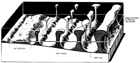
Figure 5: Diagram of different types of salt structure due to a dip at an angle of more than one degree in Northern Germany (From F. Trusheim, Bull. Amer. Assoc. Petroleum Geologists 44 (1960))

Such formation due to inclination of base rock was reported in permian salt complex of northern Germany as shown in the sketch (Fig. 5) by Trusheim [17]. Although our numerical simulation is only two-dimensional, the similarity of the formation of salt structure is rather striking. However, since the numerical data are of convenient choice only, the estimated time in million of years in numerical simulation may not be of any real significance.

Acknowledgement This work is supported by a research project from Petrobras/Brasil. The authors (ISL, MAR) also acknowledge the partial support from research fellowship of CNPq, Brazil.

References

- [1] Green, A.E.; Rivlin R.S.; Shield, R.T.: General theory of small elastic deformations superposed on finite deformations. Pro. Roy. Soc. London, Ser. A, 211, 128-154, (1952).
- [2] Liu, I-S.; Cipolatti, R.A.; Rincon, M.A.: Successive linear approximation for finite elasticity, Computational and Applied Mathematics vol. 29, no. 3, (2010).
- [3] Liu, I-S.: Successive linear approximation for boundary value problems of nonlinear elasticity in relative-descriptional formulation, Int. J. Eng Sci. (2011), doi: 10.1016/j.ijengsci.2011.02.006.
- [4] Ismail-Zadeh, A.T.; Huppert, H.E.; Lister, J.R.: Gravitational and buckling instabilities of rheologically layered structure: implications for salt diapirism, Geophys. J. Int., 148, 288-302 (2002).
- [5] van Keken, P.E.; Spiers, C.J.; van den Berg, A.P.; Muyzert, E.J.: The effective viscosity of rocksalt: implementation of steady-state creep laws in numerical models of salt diapirism, Tectonophysics, 225, 457-476 (1993).
- [6] Ciarlet, P.G.: Mathematical Elasticity, Volume. 1: Three-Dimensional Elasticity. North-Holland: Amsterdam, 1988.
- [7] Oden, J.T.: Finte Elements of Nonlinear Continua. McGraw-Hill: New York, 1972.
- [8] Ogden, R.W.: Non-Linear Elastic Deformations, Ellis Horwood: New York, 1984.
- [9] Belytschko, T.; Liu, W.K.; Moran, B.: Nonlinear Finite Elements for Continua and Structures, John Wiley & Sons: Chichester, (2000).
- [10] Simo, J.C.; Taylor, R.L.: Quasi-incompressible finite elasticity in principal stretches, continuum basis and numerical algorithms. Computer Methods in Applied Mechanics and Engineering (1991), 85: 273-310.
- [11] Simo, J.C.; Hughes, T.J.R.: Computational Inelasticity, Springer: 1998.
- [12] Zienkiewicz, O.C.; Taylor, R.L.: The Finite Element Method, Vol. 2: Solid Mechanics, Butterworth-Heinemann: Oxford, 2000.
- [13] Liu, I-S.: Continuum Mechanics, Springer: Berlin Heidelberg, 2002.
- [14] Truesdell, C.; Noll, W.: The Non-Linear Field Theories of Mechanics, 3rd edition. Springer: Berlin, 2004.
- [15] Hutter, K.; Jöhnk, K.: Continuum Methods of Physical Modeling: Continuum Mechanics, Dimensional Analysis, Turbulence, Springer, 2004.
- [16] Dixon, J.M.: Finite strain and progressive deformation in models of diapiric structures, Tectonophysics, 28, 89-124 (1975).
- [17] Trusheim, F.: Mechanism of salt migration in northern Germany, Bull. Amer. Assoc. Petroleum Geologists, 44, 1519-1540 (1960).