Inverse algorithm and M2-brane theories

Abstract

Recent paper arXiv:1103.0553 studied the quiver gauge theories on coincident $M2$ branes on a singular toric Calabi-Yau 4-folds which are complex cone over toric Fano 3-folds. There are 18 toric Fano manifolds but only 14 toric Fano were obtained from the forward algorithm. We attempt to systematize the inverse algorithm which helps in obtaining quiver gauge theories on $M2$-branes from the toric data of the Calabi-Yau 4-folds. In particular, we obtain quiver gauge theories on coincident $M2$-branes corresponding to the remaining 4 toric Fano 3-folds. We observe that these quiver gauge theories cannot be given a dimer tiling presentation.

1 Introduction

Starting with the works of Bagger-Lambert bag , Gustavsson gus , Raamsdonk ram and Aharony-Bergman-Jafferis-Maldacena (ABJM) abjm , we see interesting developments in the last three years between supersymmetric Chern-Simons gauge theory on coincident $M2$ branes at the tip of Calabi-Yau 4-folds and their string duals. For a nice review, see ref. kleb .

For a class of the supersymmetric Chern-Simons theories which can be represented by a quiver diagram, $AdS_{4}/CFT_{3}$ correspondence has been studied mar . The Calabi-Yau 4-fold toric data can be obtained for the quiver Chern-Simons theories by a procedure called forward algorithm. This approach was initially studied to obtain toric data of Calabi-Yau 3-folds from 3+1-dimensional quiver supersymmetric theories han1 . Further, if the quiver data can admit dimer tilings ken ; he1 , then the toric data can be obtained from the determinant of Kastelyne matrix. Generalising the forward algorithm/dimer tiling procedure to 2+1-dimensional quiver Chern-Simons theories resulted in obtaining toric data of many Calabi-Yau 4-folds han3 ; yama ; han4 ; han5 ; han6 ; han7a ; han7b ; han8 .

In the recent paper han8 , toric data, genus, second Betti number of 18 toric Fano 3-folds have been tabulated. We believe that there must be at least one quiver Chern-Simons theory corresponding to every toric Calabi-Yau 4-fold which are complex cones over these Fano 3-folds. Using the forward algorithm and tilings han8 , the toric data of 14 Fano 3-folds were obtained from the corresponding quiver Chern-Simons theories. Finding a quiver Chern-Simons corresponding to the remaining four toric Fanos ${\mbox{$\mathbb{P}$}}^{3},{\cal B}_{1},{\cal B}_{2},{\cal B}_{3}$ is a challenging problem which we try to attempt by systematizing the inverse algorithm.

Reversing the procedure of the forward algorithm, called inverse algorithm, should result in obtaining quiver gauge theories from the toric data. As already pointed out in the context of Calabi-Yau 3-folds han1 , the inverse algorithm has ambiguities which we will detail in section 2. Considering the toric Calabi-Yau 3-folds as embeddings inside the non-cyclic orbifolds ${\mbox{$\mathbb{C}$}}^{3}/({\mbox{$\mathbb{Z}$}}_{n}\times{\mbox{$\mathbb{Z}$}}_{m})$ and performing partial resolutions, the matter content and the superpotential $W$ of the 3+1 quiver theories were obtained han1 . However, the adjoint matter fields could not be explained by this method. The adjoint fields appear naturally in the algebraic approach tapo which involves matching matrix corresponding to dimer tiling.

Exhaustive works han3 -han8 show that all the studied quiver Chern-Simons theories corresponding to the Calabi-Yau 4-folds admit dimer tiling. Further, using higgsing han7b of matter fields on a known $G$-node quiver which admits tiling, ($G-1$) node quiver and their corresponding toric data were obtained. In fact, the approach tapo can be extended to $2+1$-dimensional quiver gauge theories giving the results in ref. han7b . All the quiver theories before or after higgsing can be represented as tiling. Unfortunately ${\mbox{$\mathbb{P}$}}^{3},{\cal B}_{1},{\cal B}_{2},{\cal B}_{3}$ toric data have not been obtained from the higgsing approach. So, we believe that these four Fano 3-folds may not give quivers admiting tiling description. It is also not clear whether we can perform partial resolution of an abelian orbifold of ${\mbox{$\mathbb{C}$}}^{4}$ han1 and obtain toric data of these Fano 3-folds.

One of the crucial step in the inverse algorithm is to fix the F-term and D-term charge assignments corresponding to the toric data. In this work, we try to understand the pattern of the F-term and the D-term charges for the 14 Fano 3-folds whose quivers are known. With this pattern identification, we propose (see ansatz in section 4.1) a form for these charges. Then, the rest of the sequence of the inverse algorithm can be performed to give the quiver data.

The plan of the paper is as follows: In section 2, we briefly review the forward and the inverse algorithm. In section 3, we first review the inverse algorithm of ${\mbox{$\mathbb{C}$}}^{4}/{\mbox{$\mathbb{Z}$}}_{2}$ which closely resembles Fano ${\mbox{$\mathbb{P}$}}^{3}$ and then derive the quiver and the mesonic moduli space Hilbert series for Fano ${\mbox{$\mathbb{P}$}}^{3}$. In section 4, we first review inverse algorithm for Fano ${\cal B}_{4}$ whose quiver is known from forward algorithm. This helps in understanding the charge assignments for the other three Fanos ${\cal B}_{1},{\cal B}_{2},{\cal B}_{3}$. We then present the details of quiver and Hilbert series for these three Fanos in later subsections. Finally, we summarize in section 5.

2 Toric data ${\cal G}\rightarrow$ quiver Chern-Simons

We will briefly discuss the inverse algorithm which is used to obtain quiver gauge theories from the toric data ${\cal G}_{4\times c}$ describing the Calabi-Yau (CY) 4-folds. Here $c$ denotes the number of points (including multiplity of points) in the toric diagram. Unlike the forward algorthim, which starts from the quiver data and superpotential $W$ giving a unique toric data, the inverse algorithm is non-unique. That is, there can be many quiver gauge theories possible from the inverse algorithm. Besides this non-uniqueness, there are many subtle ambiguities in choosing the toric data. They are:

1. Two toric data ${\cal G}$ and ${\cal G}^{\prime}$ are equivalent if they are related by any $GL(4,{\mbox{$\mathbb{Z}$}})$ transformation ${\cal T}$, that is, ${\cal G}={\cal T}.{\cal G}^{\prime}$. This leads to a huge pool of possible nullspace of ${\cal G}$ - namely, the charge matrix $Q_{(c-4)\times c}$ satisfying $Q.{\cal G}^{t}=0$ can be many.

2. The multiplicity of the toric points gives the toric data with repeated columns but they represent the same Calabi-Yau 4-folds. Usually, it is not clear which points with what multiplicity in the toric diagram to be taken. We could start with no multiplicity of all the toric points and if we end with exotic or insensible quivers, we could try putting multiplicity of some toric points. This is definitely very tedious.

We try to resolve some of these ambiquities by understanding the pattern of the matrix $Q_{(c-4)\times c}$ of the 14 toric Fano 3-folds derived from the forward algorithm han8 . We can obtain the steps of the inverse algorithm by reversing the sequence of steps in the forward algorthm.

2.1 Forward Algorithm

We will now recapitulate the essential aspects of the forward algorithm where one starts with a ${\cal N}=2$ Chern-Simons (CS) quiver gauge theory and superpotential $W$. For toric quivers, there are $N_{T}$ terms in $W$ with each matter field appearing only in two terms with opposite signs.

1. From the quiver data represented as a quiver diagram, we know the number of gauge groups $G$ (number of nodes), CS levels $k_{a}$ for each node and $m$ number of bi-fundamental matter fields and adjoints fields $X_{i}$’s. From this diagram, we can write the quiver charge matrix elements $d_{ai}$ where the index $a=1,2,\ldots G$ and $i=1,2,\ldots m$. In the CS quivers, besides $\sum_{a}d_{ai}=0$, we also require that the CS levels $k_{a}$’s have $GCD(\{k_{a}\})=1$ and $\sum_{a=1}^{G}k_{a}=0$ (Calabi-Yau requirement). Using the above conditions and the equation (moment map) of $U(1)^{G}$ abelian CS quiver gauge theories,

   $$\mu_{a}(X)=\sum_{i}d_{ai}|X_{i}|^{2}=k_{a}\sigma~{},$$ (2.1)

   where $\sigma$ is the scalar component of the vector superfield $V_{a}$, we can obtain only ($G-2$) $D$-term equations giving a projected charge matrix $\Delta_{(G-2)\times m}$ from the matrix elements $d_{ai}$. That is, the matrix elements of projected charge matrix satisfies

   $$\sum_{i}\Delta_{bi}|X_{i}|^{2}=0~{},$$ (2.2)

   where $b=1,2,\ldots(G-2)$. For example, take a $G=3$ node quiver with the the CS levels $k_{1},k_{2},-(k_{1}+k_{2})$ where $GCD(k_{1},k_{2})=1$. Further the eqns.(2.1, 2.2) suggests that the projected charge is a single row matrix whose elements are given by

   $$\Delta_{i}=k_{2}d_{1i}-k_{1}d_{2i}~{}.$$ (2.3)

2. From the F-term constraint equation $\partial W/\partial X_{i}=0$, we can obtain relations between matter fields. Introducing ($G+2$) fields $v_{r}$’s, we can incorporate the $F$-term constraints in the matrix $K_{ir}$ which relates the matter fields to $v_{i}$ in the following way:

   $$X_{i}=\prod_{r}v_{r}^{K_{ir}}$$ (2.4)

   The dual of the $K$-matrix satisfying $K.T\geq 0$ (all entries of the matrix $K.T$ are non-negative) will give a matrix $T_{(G+2)\times c}$ where $c$ gives the number of GLSM sigma model fields $p_{\alpha}$’s.

3. From the $K$ and $T$, we can write a matrix $P=K.T$. The entries of all these matrices $K$, $T$, $P$ are integers. For quiver theories which can admit tiling, one can read off $P$-matrix from $W$. The $P$-matrix relates the matter fields to GLSM $p_{\alpha}$ fields as

   $$X_{i}=\prod_{\alpha}p_{\alpha}^{P_{i\alpha}}~{}.$$ (2.5)

   The kernel of the $T$ as well as $P$ ($T.Q_{F}^{t}=P.Q_{F}^{t}=0$) will give the ${Q_{F}}_{(c-G-2)\times c}$ charge matrix.

4. From the relation (2.5), we can obtain the baryonic charge matrix ${Q_{D}}_{(G-2)\times c}$ elements from the projected charge (2.2) matrix elements as follows:

   $$\Delta_{bi}=\sum_{\alpha}P_{i\alpha}(Q_{D})_{b\alpha}~{}.$$ (2.6)

5. The total $Q$

   $$Q_{(c-4)\times c}=\left(\begin{matrix}{Q_{F}}_{(c-G-2)\times c}\cr{Q_{D}}_{(G-2)\times c}\end{matrix}\right)~{}~{},$$ (2.7)

   whose kernel $Q.{\cal G}^{t}=0$ gives the toric data ${\cal G}_{4\times c}$.

2.2 Inverse Algorithm

Now, we can reverse the sequence and try to obtain the quiver CS theory on $M2$ branes at the tip of singular CY 4-folds described by ${\cal G}$. There are additional data of toric Fano which are useful to handle some of the ambiguities we had enumerated.

1. For the toric Fano 3-folds, ${\cal G}$ can be written in a form where the symmetry of the corresponding CY 4-fold $SU(4)^{i_{1}}\times SU(3)^{i_{2}}\times SU(2)^{i_{3}}\times U(1)^{i_{4}}$ is seen as the simple roots along the rows of ${\cal G}$. As the rank of CY is 4, we require $3i_{1}+2i_{2}+i_{3}+i_{4}=4$.

2. The second betti number $b_{2}$ of the toric Fano 3-fold is related to the number of external points (E) in the toric diagram as: $b_{2}=E-3$. Further the number of baryonic symmetries for the Fano is: $b_{2}-1=E-4$. This fixes that the number of rows in the $Q_{D}$ matrix must be

   $$b_{2}-1=G-2~{}.$$ (2.8)

3. With the $GL(4,{\mbox{$\mathbb{Z}$}})$ freedom, it is not obvious as to what ${\cal G}^{\prime}$ we have to choose and find the nullspace $Q$ satisfying $Q.{\cal G}^{\prime t}=0$. However, from the eqn.(2.8), we know how many rows must represent $Q_{D}$ matrix. Equivalently, we must find a CS quiver with $G=b_{2}+1$.

4. We try to understand the pattern of $Q$ for a toric Fano with same $b_{2}$ obtained from forward algorithm and implement the same for the missing Fano 3-folds. Besides $b_{2}$, the symmetry of the Fano also suggests how to incorporate the charge assignments in the $Q$ matrix. Further, the multiplicity of points in the toric diagram is also suggested by this pattern identification. Following this methodology, we could guess a form for $Q_{F}$. Using $Q_{F}$, we determine $T$ and hence $K$.

5. The number of rows of the matrix $K$ gives the number of matter fields. From $K$, we find a relation between matter fields which are supposed to be $F$-term constraints. For the $G=(b_{2}+1)$ node quiver with the F-term constraints on the matter fields, we try to reconstruct all possible toric quiver superpotential $W$. Then we can draw the quiver diagram where the terms in $W$ must denote closed cycles in the quiver diagram.

6. Using the pattern for $Q_{D}$ from the forward algorithm for the known Fano, we can infer $Q_{D}$ charge assignment pattern for other Fano 3-folds. Further, the $Q_{D}$ must satisfy projected quiver charge (2.6). This is the non-trivial part but for small $G$, it is not difficult to find the choice of the CS levels which will give (2.3) satisfying eqn. (2.6).

In the following two sections, we will first work out the inverse algorithm for two Calabi-Yau 4-folds whose quivers are known from the tiling/forward algorithm. This will help to undersand the pattern in choosing the charge matrix $Q_{F}$ and $Q_{D}$ for the unknown Fanos ${\mbox{$\mathbb{P}$}}^{3},{\cal B}_{1},{\cal B}_{2},{\cal B}_{3}$. Using this pattern, we then perform the inverse algorithm for the missing Fano 3-folds and obtain the corresponding toric quiver CS theories. We also compute the Hilbert series and the R-charge assignments.

3 M2-brane theories from CY 4-folds with $b_{2}=1$

From the dimer tilings, we know that the number of gauge-groups is $G=2$ for the quiver gauge theory corresponding to orbifolds of ${\mbox{$\mathbb{C}$}}^{4}$ (${\mbox{$\mathbb{C}$}^{4}}/{\mbox{$\mathbb{Z}$}}_{k}$) which from eqn. (2.8) implies $b_{2}=1$. The toric Fano 3-fold ${\mbox{$\mathbb{P}$}}^{3}$ also has $b_{2}=1$. Both ${\mbox{$\mathbb{C}$}^{4}}/{\mbox{$\mathbb{Z}$}}_{k}$ and ${\mbox{$\mathbb{P}$}}^{3}$ have same number of external points in the toric diagram and hence zero baryonic symmetry: $b_{2}-1=0$. That is, $Q_{D}$ is zero. So, we expect to obtain a $G=2$ node quiver for the toric Fano ${\mbox{$\mathbb{P}$}}^{3}$ using inverse algorithm. For these Calabi-Yau 4-folds whose $Q_{D}=0$, we can directly take the matrix $T={\cal G}$ because $Q_{F}.T^{t}=Q_{F}.{\cal G}^{t}=0$. Adding multiplicity of points in the toric diagram will result in repetition of some columns of the $T$-matrix which will not alter the $K$-matrix. So, adding multiplicity of points in the toric diagram will not change the quiver data for $b_{2}=1$ CY 4-folds. We will first implement inverse algorithm for the orbifold ${\mbox{$\mathbb{C}$}}^{4}/{\mbox{$\mathbb{Z}$}}_{2}$ as a warm-up exercise and then obtain $2$-node quiver for ${\mbox{$\mathbb{P}$}}^{3}$ Fano 3-fold.

3.1 ${\mbox{$\mathbb{C}$}}^{4}/{\mbox{$\mathbb{Z}$}}_{2}$

Let us the take the toric data ${\cal G}$ for ${\mbox{$\mathbb{C}$}}^{4}/{\mbox{$\mathbb{Z}$}}_{2}$ obtained from the tiling approach (see eqn.(3.2) in ref.han7a ):

$${\cal G}=\begin{pmatrix}1&1&1&1\cr-1&0&-1&0\cr 0&-1&-1&0\cr 0&0&2&0\end{pmatrix}$$ (3.1)

As $Q_{D}=0$, we can take $T={\cal G}$. The matrix $K$ from $T$ will be

$$\begin{pmatrix}0&0&0&1\cr 0&0&-2&-1\cr 0&-2&0&-1\cr 2&2&2&1\end{pmatrix}$$ (3.2)

The row index of the $4\times 4$ square matrix $K$ indicates that the number of matter fields in the quiver theory is $4$ confirming the known data for ${\mbox{$\mathbb{C}$}}^{4}$ orbifolds. Also, being a square matrix, it is not possible to find $F$-term constraint equations. From the matter field content, one can try to construct all possible connected quiver diagrams and the loops in the quiver diagram will give gauge invariant terms in superpotential $W$. The information about the Chern-Simons level $k_{a}$ is inferred from the matrix $P=K.T$ which for this case is given as:

$$P=\begin{pmatrix}0&0&2&0\cr 0&2&0&0\cr 2&0&0&0\cr 0&0&0&2\end{pmatrix}$$ (3.3)

For ${\mbox{$\mathbb{C}$}}^{4}$, the $P$ matrix from inverse algorithm will turn out to have entries zero or 1. So, the entries for ${\mbox{$\mathbb{C}$}}^{4}/{\mbox{$\mathbb{Z}$}}_{2}$ which are $2$ or $0$ indicates that one of the nodes of the 2-node quiver diagram must have level $k_{1}=2$ and the other node by Calabi-Yau requirement has level $k_{2}=-k_{1}=-2$. Inferring the CS levels from $P$-matrix is only applicable for CY 4-folds whose $Q_{D}=0$. The $Q_{F}$ satisfying $P.Q_{F}^{t}=0$ is also trivial.

Hence from the inverse algorithm for ${\mbox{$\mathbb{C}$}}^{4}/{\mbox{$\mathbb{Z}$}}_{2}$, there can be three possible 2-node quivers with four matter fields and levels $k_{1}=-k_{2}=2$. They are:

1. ABJM theory with 4 bi-fundamental matter fields $X_{12}^{i}$ and $X_{21}^{i}$ where $i=1,2$ and $W=Tr[\epsilon_{ij}X_{12}^{1}X_{21}^{i}X_{12}^{2}X_{21}^{j}]$ whose abelian $W=0$.

2. 2-node quiver with two adjoints $\phi_{2}^{1},\phi_{2}^{2}$ at the same node (say node 2) and two bifundamentals $X_{12},X_{21}$. Here $W=Tr[X_{12}[\phi_{2}^{1},\phi_{2}^{2}]X_{21}]$ whose abelian $W$ is again zero.

3. 2-node quiver with two bifundamentals $X_{12}$,$X_{21}$ and adjoints $\phi_{1}$ and $\phi_{2}$ at two different nodes with trivial $W=0$.

It is important to realise that it is not possible to do forward algorithm for quivers whose abelian superpotential $W$ is zero. Particularly, we cannot obtain the matrix $K$ for these superpotentials. Fortunately, the first two quivers admit dimer tiling presentation han3 . So, we can obtain toric data ${\cal G}$ directly from the determinant of the Kastelyne matrix. We would also like to point out that the $P$ matrix obtained from $W$ is same for ${\mbox{$\mathbb{C}$}}^{4}$ and ${\mbox{$\mathbb{C}$}}^{4}/{\mbox{$\mathbb{Z}$}}_{2}$ indicating that the $P$ matrix does not give information about the Chern-Simon levels. From inverse algorithm, we actually find the $P$-matrix entries change with change in CS levels.

Comparing the tiling approach and the inverse algorithm, we infer that third quiver is not allowed for ${\mbox{$\mathbb{C}$}}^{4}/{\mbox{$\mathbb{Z}$}}_{2}$. We will see a similar situation arising in the following section on Fano ${\mbox{$\mathbb{P}$}}^{3}$.

3.2 Fano ${\mbox{$\mathbb{P}$}}^{3}$ theory

The symmetry group of the Calabi-Yau 4-folds constructed as complex cone over Fano ${\mbox{$\mathbb{P}$}}^{3}$ is $SU(4)\times U(1)$. Further $b_{2}=1$ implies $G=2$-node quiver and $Q_{D}=0$. Therefore, the matrix $T={\cal G}$ where the toric data ${\cal G}_{4\times c}$ respecting the symmetry is:

$$\begin{pmatrix}1&1&1&1&1\cr 1&-1&0&0&0\cr 0&1&-1&0&0\cr 0&0&1&-1&0\end{pmatrix}$$ (3.4)

Here the number of points in the toric diagram $c=5$ and hence $(Q_{F})_{(c-4)\times c}$ will be a single row with five entries. The first four columns in ${\cal G}$ are the external points and the last column denotes the internal point in the toric diagram.

For the given symmetry $SU(4)\times U(1)$, we can always choose the fermionic charge assignment $Q_{F}=(aaaab)$ where $a,b$ are integers. Further $Q_{F}.{\cal G}^{t}=0$ implies $4a+b=0$. Conversely, the charge $Q_{F}$ with four entries same reflects that the Calabi-Yau 4-fold has $SU(4)$ symmetry. The possible choice of $a,b$ in $Q_{F}$ is

$$Q_{F}=(1,1,1,1,-4)~{}.$$ (3.5)

The matrix $K$ such that $(K.T)\geq 0$ turns out be again a $4\times 4$ matrix.

$$\begin{pmatrix}1&-1&-2&-3\cr 1&-1&-2&1\cr 1&-1&2&1\cr 1&3&2&1\end{pmatrix}$$

So, for the toric data for ${\mbox{$\mathbb{P}$}}^{3}$, the $K$-matrix implies that the number of matter fields must be again 4 which is consistent with eqn. (2.8).

As the toric data ${\cal G}$ for ${\mbox{$\mathbb{P}$}}^{3}$ is not related to toric data of the orbifold ${\mbox{$\mathbb{C}$}}^{4}/{\mbox{$\mathbb{Z}$}}_{k}$ by $GL(4,{\mbox{$\mathbb{Z}$}})$, we would expect that the corresponding $K$-matrices are not related by the $GL(4,{\mbox{$\mathbb{Z}$}})$ and it is indeed true. Therefore, the quiver for ${\mbox{$\mathbb{P}$}}^{3}$ toric data has to be different from the quiver for ${\mbox{$\mathbb{C}$}}^{4}/{\mbox{$\mathbb{Z}$}}_{k}$ toric data.

The matching matrix $P=K.T$ is given by:

$$P=\begin{pmatrix}0&0&0&4&1\cr 0&0&4&0&1\cr 0&4&0&0&1\cr 4&0&0&0&1\end{pmatrix}$$ (3.6)

We see that the non-zero entries in the first four columns corresponding to the external points of ${\mbox{$\mathbb{P}$}}^{3}$ toric diagram is 4. Following our results on ${\mbox{$\mathbb{C}$}}^{4}/{\mbox{$\mathbb{Z}$}}_{2}$, it appears that the levels of the quiver CS theory with four matter fields will be $k_{1}=-k_{2}=4$.

The quiver corresponding to ${\mbox{$\mathbb{P}$}}^{3}$ must be a 2-node quiver with 4 matter fields with levels $k_{1}=-k_{2}=4$, which can again have three possibilities. Two of the quivers corresponds to ${\mbox{$\mathbb{C}$}}^{4}/{\mbox{$\mathbb{Z}$}}_{4}$ from the tiling approach han3 . By the elimination process, we claim that the quiver drawn in figure 1 represents the quiver gauge theory on the coincident $M2$ branes at the tip of the singular Calabi-Yau, which is complex cone over Fano ${\mbox{$\mathbb{P}$}}^{3}$ with superpotential $W=0$.

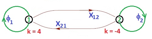
Figure 1: Quiver Diagram for Fano $P^{3}$

All the studied quivers with $N_{T}$ terms in $W$, $G$ nodes and $E$ edges satisfied $N_{T}-E+G=0$ and hence could be drawn as tiling on a two-torus han3 ; han4 ; han5 ; han6 ; han7a ; han7b . This quiver satisfies $N_{T}-E+G=-2$. It will be interesting to see whether this quiver could admit a $3d$ tiling which will help to obtain the Kastelyne matrix and the toric data sang ; sang1 . We also believe that this quiver must be obtainable by the Higgsing of some quiver gauge theory, which does not admit tiling presentation, with three gauge group nodes.

Taking the $Q_{F}$ (3.5) for the toric data ${\cal G}$, we will work out the Hilbert series of the mesonic moduli space. As this Fano has only one $U(1)$ charge, which can be taken as R-charge, the Hilbert series must have the following expected form:

$$g^{\rm mes}(t;X)=\frac{1+(g-2)t+(g-2)t^{2}+t^{3}}{(1-t)^{4}}~{}.$$ (3.7)

where $X$ denotes Fano 3-fold of genus $g$. Following Ref. han8 , we will take the $R$-charge fugacity of the four external points as $s_{1}$ and for the internal point as 1. Then the Hilbert series (3.7) for this case will come out to be:

$$g^{mes}(s_{1},{\mbox{$\mathbb{P}$}}^{3}) = \oint_{|z|=1}\frac{dz}{2\pi iz}\frac{1}{(1-s_{1}z)^{4}(1-z^{-4})}$$

$$= \frac{(1+31z^{4}+31z^{8}+z^{12})}{(z^{4}-1)^{4}}|_{z=1/s_{1}}$$ (3.8)

Excluding the poles on the boundary of the contour, we indeed get the expected form (3.7) with the correct genus $g=33$ confirming that the charge assignment and the toric data we considered (with no multiplicity) is correct.

We will now try to understand the inverse algorithm for other Fano 3-folds whose $b_{2}=2$ in the following section.

4 M2-brane theories from CY 4-folds with $b_{2}=2$

There are four toric Fano 3-folds ${\cal B}_{i}$ whose second Betti number $b_{2}=2$. They have $E=5$ external points and one internal point in the toric diagram. From the tiling/forward algorithm, Fano ${\cal B}_{4}$ toric data and hilbert series were derived from a $G=3$ node quiver gauge theory. As ($b_{2}-1)=(E-4)=(G-2)=1$ for all these Fano ${\cal B}_{i}$’s, we expect to obtain $G=3$ node quivers from the inverse algorithm. Further, the number of baryonic symmetries is $(b_{2}-1)=1$ for these Fano 3-folds. So, $Q_{D}$ matrix will be a single row matrix.

In order to understand the pattern of $Q_{F}$ and $Q_{D}$ matrix, we will first do the inverse algorithm for the Fano ${\cal B}_{4}$ and obtain the same $3$-node quiver known from the tiling/forward algorithm. Then, we will repeat the similar $Q$-charge pattern for the other three Fano 3-folds and obtain their corresponding 3-node quiver gauge theories.

4.1 Fano $\mathcal{B}_{4}$ theory

The CY 4-fold obtained from the complex cone over ${\cal B}_{4}$ has $SU(3)\times SU(2)\times U(1)$ symmetry. The toric data ${\cal G}$ which reflects this symmetry is

$$G=\begin{pmatrix}1&1&1&1&1&1\cr 1&-1&0&0&0&0\cr 0&1&-1&0&0&0\cr 0&0&0&1&-1&0\end{pmatrix}~{}.$$ (4.1)

For the Fano with the given symmetry, the $Q$ matrix must have first three columns are identical, fourth and fifth column to be identical. Observing the $Q$-charge pattern for the 14-toric Fano from the tiling/forward algorithm, we propose the following:
Ansatz: $Q_{F}$ matrix columns must possess non-abelian symmetry whose rank is one higher than that of the $Q_{D}$ matrix. Further, the ranks of the non-abelian subgroups in $Q_{F}$ must be atmost the maximal rank of the subgroups representing the symmetry of the toric CY 4-folds.
This proposal helps in fixing the multiplicity of the points in the toric diagram as well. For ${\cal B}_{4}$, $Q_{F}$ matrix must have $SU(3)\times SU(3)$ symmetry. That is, the integer entries of the $Q_{F}$ matrix must be:

$${Q_{F}}_{(c-G-2)\times c}=\begin{pmatrix}a_{1}&a_{1}&a_{1}&b_{1}&b_{1}&b_{1}&c_{1}&d_{1}\ldots\cr a_{2}&a_{2}&a_{2}&b_{2}&b_{2}&b_{2}&c_{2}&d_{2}\ldots\cr.&.&.&&&&&\ldots\cr.&.&.&&&&&\ldots\cr a_{c-5}&a_{c-5}&a_{c-5}&b_{c-5}&b_{c-5}&b_{c-5}&c_{c-5}&d_{c-5}\ldots\end{pmatrix}~{},$$ (4.2)

where the $\ldots$ denotes possible multiplicities of the points in the toric diagram. The single row $Q_{D}$ entries must have $SU(3)\times SU(2)\times U(1)$:

$${Q_{D}}_{1\times c}=\left(\begin{matrix}x&x&x&y&y&l&m\ldots\end{matrix}\right)$$ (4.3)

so that the total $Q$ possesses the symmetry of the Fano ${\cal B}_{4}$.

For the given ${\cal G}$ with no multiplicity, we are able to find a $Q_{F}$ and $Q_{D}$ obeying the above pattern:

$$Q=\begin{pmatrix}Q_{F}\cr Q_{D}\end{pmatrix}=\begin{pmatrix}1&1&1&-1&-1&-1\cr 0&0&0&1&1&-2\end{pmatrix}$$ (4.4)

The $T$ and $K$ matrix for this choice of $Q_{F}$ is:

$$T=\begin{pmatrix}1&0&0&0&0&1\cr 1&0&0&0&1&0\cr 1&0&0&1&0&0\cr-1&0&1&0&0&0\cr-1&1&0&0&0&0\end{pmatrix}~{};~{}K=\left(\begin{array}[]{c|ccccc}{}\hfil&v_{1}&v_{2}&v_{3}&v_{4}&v_{5}\\ \hline\cr X_{12}^{(1)}&0&0&1&0&0\\ X_{12}^{(2)}&0&0&1&0&1\\ X_{12}^{(3)}&0&0&1&1&0\\ X_{23}^{(1)}&0&1&0&0&0\\ X_{23}^{(2)}&0&1&0&0&1\\ X_{23}^{(3)}&0&1&0&1&0\\ X_{31}^{(1)}&1&0&0&0&0\\ X_{31}^{(2)}&1&0&0&0&1\\ X_{31}^{(3)}&1&0&0&1&0\end{array}\right)$$ (4.5)

From the $K$-matrix, we know that the number of matter fields is $9$. We can also reconstruct toric superpotential $W$ using the $F$-term constraints given by the $K$-matrix:

$$W={\rm Tr}\left(\epsilon_{ijk}X_{12}^{(i)}X_{23}^{(j)}X_{31}^{(k)}\right)~{}$$ (4.6)

and draw the $3$-node cyclic quiver where the matter fields $X_{ij}^{(l)}$’s are bifundamental fields from the node $i$ to the node $j$ which will determine the quiver charge matrix:

$$d=\left(\begin{array}[]{c|c c c}&X_{12}^{(i)}&X_{23}^{(j)}&X_{31}^{(k)}\\ \hline\cr a=1&1&0&-1\\ a=2&-1&1&0\\ a=3&0&-1&1\end{array}\right)$$ (4.7)

In order to determine the CS levels $k_{a}$’s, we have to write the $P=K.T$ matrix:

$$P=\left(\begin{array}[]{c|cccccc}&p_{1}&p_{2}&p_{3}&p_{4}&p_{5}&p_{6}\\ \hline\cr X_{12}^{(1)}&1&0&0&1&0&0\\ X_{12}^{(2)}&0&1&0&1&0&0\\ X_{12}^{(3)}&0&0&1&1&0&0\\ X_{23}^{(1)}&1&0&0&0&1&0\\ X_{23}^{(2)}&0&1&0&0&1&0\\ X_{23}^{(3)}&0&0&1&0&1&0\\ X_{31}^{(1)}&1&0&0&0&0&1\\ X_{31}^{(2)}&0&1&0&0&0&1\\ X_{31}^{(3)}&0&0&1&0&0&1\end{array}\right)~{},$$ (4.8)

where we have again indicated the matter fields which represent the row index and the GLSM $p_{\alpha}$ denoting the column index which will help to write these matter fields as products of GLSM $p_{\alpha}$ fields. Using the $Q_{D}$ charge (4.4) and the $P$-matrix elements, we can obtain the projected charge $\Delta$ of the matter fields (2.6):

$$\Delta=\left(\begin{array}[]{ccc}X_{12}^{(1,2,3)}&X_{23}^{(1,2,3)}&X_{31}^{(1,2,3)}\\ \hline\cr 1&1&-2\end{array}\right)$$ (4.9)

Substituting the projected charge and the $d$-matrix elements (4.7) in eqn.(2.3), we find that the CS levels have to be

$$k_{1}=1~{},~{}k_{2}=-2~{},k_{3}=1~{}.$$ (4.10)

Thus, using inverse algorithm with a possible choice of $Q$ matrix respecting the ansatz on the $Q_{F},Q_{D}$ pattern, we have obtained the same $3$-node quiver CS theory with $W$, CS levels and $\Delta$ charge han8 confirming that the inverse algorithm is agreeing with the forward algorithm for the Fano ${\cal B}_{4}$. Now, we are in a position to extend this pattern approach for other ${\cal B}_{i}$ Fano 3-folds and obtain the corresponding quiver CS theories. The Hilbert series of the mesonic moduli space worked out in ref. han8 involves taking a simple pole or irrational pole in each of the two integration variables to the boundary of the contour by scaling the variables. Evaluating the contour in the scaled variables and excluding the poles at the boundary gives the form (3.7) agreeing with the genus $g=28$.

4.2 Fano ${\cal B}_{1}$ theory

The symmetry possessed by this ${\cal B}_{1}$ Fano is $SU(3)\times U(1)^{2}$. Using our ansatz, we need to choose $Q_{F}$ to have $SU(3)\times SU(2)\times U(1)$ symmetry. This could not be achieved without taking multiplicity of the points in the toric diagram. Hence, we start with the following toric data:

$${\cal G}=\left(\begin{array}[]{ccccccc}1&1&1&1&1&1&1\\ 1&-1&0&0&0&0&0\\ 0&1&-1&0&0&0&0\\ 0&0&2&-1&1&1&0\end{array}\right)$$ (4.11)

where we have taken multiplicity of an external point which is shown as repeated columns 5 and 6 in ${\cal G}$. The last column represents the internal point in the toric diagram. The $Q_{F}$ matrix will have now 2 rows and can be taken, following ansatz, as:

$$Q_{F}=\left(\begin{array}[]{ccccccc}1&1&1&-2&-2&-2&3\\ 0&0&0&2&1&1&-4\end{array}\right)$$ (4.12)

We can take a possible choice for the single row $Q_{D}$ imposing its entries so that the $Q$ matrix respect $SU(3)\times U(1)^{2}$ symmetry:

$$Q_{D}=\left(\begin{array}[]{ccccccc}0,&0,&0,&1,&0,&1,&-2\end{array}\right)$$ (4.13)

With this $Q_{F}$, we can find $T$ and hence the $K$ matrix as:

$$T=\begin{pmatrix}1&0&0&2&0&0&1\cr 2&0&0&-1&0&2&0\cr 2&0&0&-1&2&0&0\cr-1&0&1&0&0&0&0\cr-1&1&0&0&0&0&0\end{pmatrix}~{};~{}K=\left(\begin{array}[]{c|ccccc}{}\hfil&v_{1}&v_{2}&v_{3}&v_{4}&v_{5}\\ \hline\cr X_{1}&1&0&0&0&0\\ X_{2}&1&0&0&0&1\\ X_{3}&1&0&0&1&0\\ X_{4}&1&0&2&0&0\\ X_{5}&1&0&2&0&5\\ X_{6}&1&0&2&5&0\\ X_{7}&1&2&0&0&0\\ X_{8}&1&2&0&0&5\\ X_{9}&1&2&0&5&0\end{array}\right)$$ (4.14)

The $K$-matrix indicates that there are $9$ matter fields $X_{i}$’s. From the $K$-matrix, we do find the following relations: $X_{9}X_{4}=X_{6}X_{7},~{}X_{5}X_{9}=X_{6}X_{8},~{}X_{5}X_{7}=X_{4}X_{8},$ and we could construct a toric superpotential $W$ respecting the above equation as $W={\rm Tr}\left[X_{1}(X_{5}X_{9}-X_{6}X_{8})-X_{2}(X_{5}X_{7}-X_{4}X_{8})+X_{3}(X_{6}X_{7}-X_{9}X_{4})\right]~{}.$
However, the F-term constraint $\partial W\over\partial X_{i}$ for $X_{4},X_{5},\ldots X_{9}$ is not respected by the $K$-matrix. Hence the only possible toric superpotential $W$ will be a two-term superpotential with each term involving all the $9$ matter fields:

$$W={\rm Tr}\left[X_{2}X_{5}X_{8}\{X_{1}X_{4}X_{9}X_{3}X_{6}X_{7}-X_{1}X_{6}X_{7}X_{3}X_{4}X_{9}\}\right]~{}.$$ (4.15)

Clearly, abelian $W=0$ and hence we cannot perform forward algorithm for this $3$-node quiver. Further $N_{T}-E+G=2-9+3=-4$ and hence cannot admit tiling presentation.

The $W$ suggests the 3-node quiver must be as shown in figure 2. From the quiver diagram, we can obtain the $d$-matrix elements:

$$d_{ai}=\left(\begin{array}[]{c|ccc}&X_{i}(i=1,2,3)&X_{i}(i=4,5,6)&X_{i}(i=7,8,9)\\ \hline\cr a=1&-1&1&0\\ a=2&0&-1&1\\ a=3&1&0&-1\end{array}\right)$$ (4.16)

To determine the CS levels of the three nodes, we need the $P=K.T$ matrix:

$$P=\left(\begin{array}[]{ccccccc}1&0&0&2&0&0&1\\ 0&1&0&2&0&0&1\\ 0&0&1&2&0&0&1\\ 5&0&0&0&4&0&1\\ 0&5&0&0&4&0&1\\ 0&0&5&0&4&0&1\\ 5&0&0&0&0&4&1\\ 0&5&0&0&0&4&1\\ 0&0&5&0&0&4&1\end{array}\right)$$ (4.17)

Using the above matrix elements and the $Q_{D}$ (4.13), we obtain the following $\Delta$ charge for the nine-matter fields in the $G=3$ node quiver:

$$\Delta=\left(\begin{array}[]{ccc}X_{1,2,3}&X_{4,5,6}&X_{7,8,9}\\ \hline\cr 0&-2&2\end{array}\right)$$ (4.18)

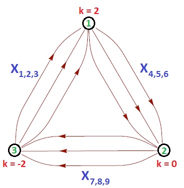
Figure 2: ${\cal B}_{1}$ Quiver Diagram

Substituting $\Delta$ charge (4.18) and $d$ charge (4.16) in eqn.(2.3), we find that the CS levels of the three nodes must be

$$k_{1}=2~{},k_{2}=0~{},k_{3}=-2~{}.$$ (4.19)

As a further consistent check with our charge assignment (4.12, 4.13), we will work out the Hilbert series for the mesonic moduli space in the following subsection.

4.2.1 Hilbert series for ${\cal B}_{1}$ Theory

The total charge matrix for the ${\cal B}_{1}$ theory (4.12, 4.13) is

$$Q=\left(\begin{array}[]{c}Q_{F}\\ Q_{D}\end{array}\right)=\left(\begin{array}[]{ccccccc}p_{1}&p_{2}&p_{3}&p_{4}&p_{5}&\tilde{p}_{5}&p_{6}\\ \hline\cr 1&1&1&-2&-2&-2&3\\ 0&0&0&2&1&1&-4\\ 0&0&0&1&0&1&-2\end{array}\right)$$ (4.20)

Here, we have $c=7$ $p_{\alpha}$ fields. Let us denote the R-charge fugacity associated with the first three $p_{\alpha}$’s ($p_{1},p_{2},p_{3}$) respecting $SU(3)$ symmetry as $s_{1}$ and fugacities associated with $p_{4}$, $p_{5}$ and ${\tilde{p}}_{5}$ as $s_{2}$, $s_{3}$ and $s_{4}$ respectively. Since the R-charge of the internal point $p_{6}$ is 0, the corresponding fugacity is set to unity. Using the $Q$ matrix, the Hilbert series of the mesonic moduli space can be written as:

$$g^{mes}(s_{1},s_{2},s_{3},s_{4};{\cal B}_{1}) = \oint_{|z_{1}|=1}\left(\frac{\text{$dz_{1}$}}{2\pi\text{$\mathit{i}$$z_{1}$}}\right)\oint_{|z_{2}|=1}\left(\frac{\text{$dz_{2}$}}{2\pi\text{$\mathit{i}$$z_{2}$}}\right)\oint_{|b|=1}\left(\frac{db}{2\pi\text{$\mathit{i}$$b$}}\right)$$

$$\left\{\frac{1}{\left(1-s_{1}z_{1}\right)^{3}\left(1-s_{2}\frac{bz_{2}^{2}}{z_{1}^{2}}\right)\left(1-s_{3}\frac{z_{2}}{z_{1}^{2}}\right)\left(1-s_{4}\frac{z_{2}b}{z_{1}^{2}}\right)\left(1-\frac{z_{1}^{3}}{b^{2}z_{2}^{4}}\right)}\right\}$$

Similar to the ${\cal B}_{4}$ integration, we have scaled each integration variable so that the simple pole (preferably irrational pole) is on the boundary. Evaluating the integration with the above scaling, we obtain

$$g^{mes}(s_{1},s_{2},s_{3},s_{4};{\cal B}_{1}) = \frac{s_{3}s_{4}}{\left(s_{1}^{5}s_{3}^{2}s_{4}^{2}-1\right)^{3}\left(s_{2}^{5}-s_{3}s_{4}\right)}\left\{1+3s_{1}s_{2}^{2}+6s_{1}^{2}s_{2}^{4}\right.$$

$$~{}~{}~{}\left.+10s_{1}^{3}s_{2}s_{3}s_{4}+15s_{1}^{4}s_{2}^{3}s_{3}s_{4}+18s_{1}^{5}s_{3}^{2}s_{4}^{2}+19s_{1}^{6}s_{2}^{2}s_{3}^{2}s_{4}^{2}\right.$$

$$~{}~{}\left.+18s_{1}^{7}s_{2}^{4}s_{3}^{2}s_{4}^{2}+15s_{1}^{8}s_{2}s_{3}^{3}s_{4}^{3}+10s_{1}^{9}s_{2}^{3}s_{3}^{3}s_{4}^{3}+6s_{1}^{10}s_{3}^{4}s_{4}^{4}\right.$$

$$\quad\left.+3s_{1}^{11}s_{2}^{2}s_{3}^{4}s_{4}^{4}+s_{1}^{12}s_{2}^{4}s_{3}^{4}s_{4}^{4}\right\}$$ (4.21)

Let us define two new fugacities, $t_{1}\equiv s_{1}^{1/2}s_{3}^{1/5}s_{4}^{1/5}$ and $t_{2}\equiv s_{2}s_{3}^{-1/5}s_{4}^{-1/5}$. So, the Hilbert series for mesonic moduli space will be given as:

$$g^{mes}(t_{1},t_{2};{\cal B}_{1}) = \frac{1}{\left(1-t_{2}^{5}\right)\left(1-t_{1}^{10}\right)^{3}}\left\{1+10t_{2}t_{1}^{6}+15t_{2}t_{1}^{16}+3t_{2}^{2}t_{1}^{2}+6t_{2}^{4}t_{1}^{4}\right.$$

$$~{}~{}\left.+15t_{2}^{3}t_{1}^{8}+18t_{1}^{10}+19t_{2}^{2}t_{1}^{12}+18t_{2}^{4}t_{1}^{14}+10t_{2}^{3}t_{1}^{18}+6t_{1}^{20}\right.$$

$$\left.+3t_{2}^{2}t_{1}^{22}+t_{2}^{4}t_{1}^{24}\right\}~{}.$$ (4.22)

This is the expected polynomial form for the Calabi-Yau 4-folds with $U(1)^{2}$ symmetry. This indirectly confirms that our charge assignment (4.20) is correct. We can determine the $R$-charge assignment of the $p_{\alpha}$ fields following the steps in ref. han8 . Suppose, $R_{1}$ and $R_{2}$ be the R-charges corresponding to the fugacities $t_{1}$ and $t_{2}$. That is, $t_{1}=e^{-\mu R_{1}}$ and $t_{2}=e^{-\mu R_{2}}$, where $\mu$ is the chemical potential for the R-charge. So, the volume of ${\cal B}_{1}$ will be given as:

$$V({\cal B}_{1})=\lim_{\mu\to 0}\mu^{4}g^{mes}(e^{-\mu R_{1}},e^{-\mu R_{2}};{\cal B}_{1})~{}.$$ (4.23)

However, $R_{1}$ and $R_{2}$ are not independent. Using the terms in the superpotential (4.15) to have $R$-charge 2 implies that the product of all the matter fields which in terms of $p_{\alpha}$ fields from $P$ matrix (4.17) ($\prod\limits_{i=1}^{9}X_{i}=p_{1}^{11}p_{2}^{11}p_{3}^{11}p_{4}^{6}p_{5}^{12}p_{6}^{12}p_{7}^{9}$) must have $R$-charge 2 which implies that:

$$33R_{1}+3R_{2}=1$$ (4.24)

Putting it in volume of ${\cal B}_{1}$ (4.23) and minimising it, we get $\hat{R}_{1}=0.02272$ and $\hat{R}_{2}=0.08333$. The R-charge of the $p_{\alpha}$ field can be found by using:

$$R(p_{\alpha})=\lim_{\mu\to 0}\frac{1}{\mu}\left[\frac{g(e^{-\mu\hat{R}_{i}};D_{\alpha})}{g^{mes}(e^{-\mu\hat{R}_{i}};{\cal B}_{1})}-1\right]$$ (4.25)

where $D_{\alpha}$ is the divisor corresponding to the field $p_{\alpha}$ and $g(e^{-\mu\hat{R}_{i}};D_{\alpha})$ gives the associated Hilbert series evaluated at the $\hat{R}_{i}$ which minimises $V({\cal B}_{1})$. For the given charge assignment (4.20), the associated Hilbert series for the divisor $D_{1}$ corresponding to the field $p_{1}$ is

$$g(s_{1},s_{2},s_{3},s_{4};D_{1}) = \oint_{|z_{1}|=1}\left(\frac{\text{$dz_{1}$}}{2\pi\text{$\mathit{i}$$z_{1}$}}\right)\oint_{|z_{2}|=1}\left(\frac{\text{$dz_{2}$}}{2\pi\text{$\mathit{i}$$z_{2}$}}\right)\oint_{|b|=1}\left(\frac{db}{2\pi\text{$\mathit{i}$$b$}}\right)$$

$$\left\{\frac{{(s_{1}z_{1})}^{-1}}{\left(1-s_{1}z_{1}\right)^{3}\left(1-s_{2}\frac{bz_{2}^{2}}{z_{1}^{2}}\right)\left(1-s_{3}\frac{z_{2}}{z_{1}^{2}}\right)\left(1-s_{4}\frac{z_{2}b}{z_{1}^{2}}\right)\left(1-\frac{z_{1}^{3}}{b^{2}z_{2}^{4}}\right)}\right\}$$

The $SU(3)$ symmetry of the ${\cal B}_{1}$ requires $R(p_{1})=R(p_{2})=R(p_{3})$. Substituting the fugacities $s_{1},s_{2},s_{3},s_{4}$ and rewriting in terms of $t_{1},t_{2}$, the $R$-charge of $p_{1}$ field turns out to be $R(p_{1})=2\hat{R}_{1}$. Similarly, computation of associated Hilbert series for divisor $D_{4}$ corresponding to field $p_{4}$ gives $R(p_{4})=\hat{R}_{2}$. This method enables evaluation of $R$-charges of all the $p_{\alpha}$ fields. In fact, $R(p_{5})=R(p_{6})=0$.

We know that ${\cal B}_{1}$ has two $U(1)$ symmetries. We have found $R$-charge corresponding to one $U(1)$ symmetry. The $q$-charge assignment, corresponding to the other abelian mesonic symmetry $U(1)$, must be such that the superpotential terms (4.15) are uncharged. Further the $q$-charge vector must be linearly independent to $Q_{F},Q_{D}$ (4.20). We have tabulated all these results in Table 1.

	$SU(3)$	$U(1)_{R}$	$U(1)_{B}$	$U(1)_{q}$	fugacity
$p_{1}$	(1,0)	0.04545	0	1	$s_{1}y_{1}q$
$p_{2}$	(1-,1)	0.04545	0	1	$s_{1}y_{2}q/y_{1}$
$p_{3}$	(0,-1)	0.04545	0	1	$s_{1}q/y_{2}$
$p_{4}$	(0,0)	0.08333	1	-1	$s_{2}b/q$
$p_{5}$	(0,0)	0	0	-3	$1/q^{3}$
${\tilde{p}}_{5}$	(0,0)	0	1	0	$b$
$p_{6}$	(0,0)	0	-2	1	$q/b^{2}$

Table 1: Various charges of $p_{\alpha}$ fields under global symmetry of ${\cal B}_{1}$ theory. In this table, $s_{i}$ are the fugacities of R-charges, $y_{1}$ and $y_{2}$ are weights of $SU(3)$ symmetry, $b$ and $q$ are fugacities of $U(1)_{B}$ and $U(1)_{q}$ symmetries respectively.

4.3 Fano ${\cal B}_{2}$ theory

The symmetry of ${\cal B}_{2}$ is also $SU(3)\times U(1)^{2}$. So, we expect, from anatz, $Q_{F}$ charge assignmnet to respect $SU(3)\times SU(2)\times U(1)$. In order to achieve this symmetry, we take multiplicity of two external points $p_{4},p_{5}$ in the toric diagram giving the following toric data:

$${\cal G}=\left(\begin{array}[]{ccccccccc}&p_{1}&p_{2}&p_{3}&p_{4}&{\tilde{p}}_{4}&p_{5}&{\tilde{p}}_{5}&p_{6}\\ \hline\cr&1&1&1&1&1&1&1&1\\ &1&-1&0&0&0&0&0&0\\ &0&1&-1&0&0&0&0&0\\ &0&0&1&-1&-1&1&1&0\end{array}\right)$$ (4.27)

and we choose the following $Q_{F}$ charge matrix with first three columns identical, fourth and sixth column identical so that the non-abelian symmetry $SU(3)\times SU(2)$ is obeyed:

$$Q_{F}=\left(\begin{array}[]{cccccccc}1&1&1&-1&-1&-1&-2&2\\ 0&0&0&1&-1&1&-1&0\\ 0&0&0&0&1&0&1&-2\end{array}\right)$$ (4.28)

A possible choice for the baryonic charge $Q_{D}$ matrix with breaks the symmetry to $SU(3)\times U(1)^{2}$ is:

$$Q_{D}=\left(\begin{array}[]{cccccccc}0,&0,&0,&1,&1,&2,&0,&-4\end{array}\right)$$ (4.29)

From $Q_{F}$ charge assignment (4.28), we can find the $T$ and hence the $K$ matrix as:

$$T=\begin{pmatrix}2&0&0&2&2&0&0&1\cr 1&0&0&0&-1&0&1&0\cr 0&0&0&-1&0&1&0&0\cr-1&0&1&0&0&0&0&0\cr-1&1&0&0&0&0&0&0\end{pmatrix}~{};~{}K=\left(\begin{array}[]{ccccc}1&0&0&0&0\\ 1&0&0&0&2\\ 1&0&0&2&0\\ 1&0&2&0&0\\ 1&0&2&0&2\\ 1&0&2&2&0\\ 1&2&0&0&0\\ 1&2&0&0&4\\ 1&2&0&4&0\\ 1&2&2&0&0\\ 1&2&2&0&4\\ 1&2&2&4&0\end{array}\right)$$ (4.30)

Here, the rows denote the matter fields $X_{i}$, ($i=1,2,...,12$). From the $K$ matrix elements, we can construct a toric superpotential $W$ as

$$W = {\rm Tr}\left(X_{1}X_{4}X_{8}X_{12}-X_{1}X_{4}X_{9}X_{11}-X_{2}X_{5}X_{7}X_{12}\right.$$

$$\left.+X_{2}X_{5}X_{9}X_{10}+X_{3}X_{6}X_{7}X_{11}-X_{3}X_{6}X_{8}X_{10}\right)~{}.$$ (4.31)

           

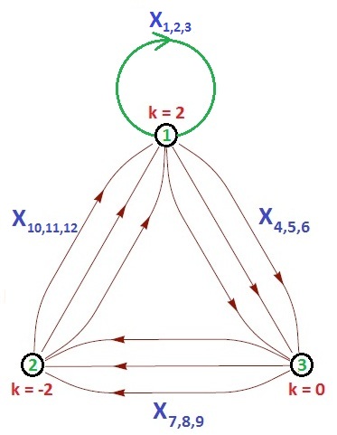
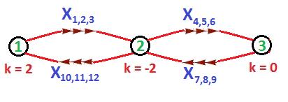
Figure 3: Two quivers (1) and (2) for the ${\cal B}_{2}$ toric data

There are $N_{T}=6$ terms in $W$ for the $G=3$ node quiver with $E=12$ matter fields. Clearly, $N_{T}-E+G=-3$ and cannot admit tiling presentation. However, the abelian $W$ is non-zero. So, it must be possible to do the forward algorithm after deducing the quiver diagram with CS levels from the inverse algorithm. This suggests two possible quivers as shown in figure 3.

To obtain the CS levels on the three nodes of the quiver, we need the matrix $P=K.T$:

$$P=\left(\begin{array}[]{cccccccc}2&0&0&2&2&0&0&1\\ 0&2&0&2&2&0&0&1\\ 0&0&2&2&2&0&0&1\\ 2&0&0&0&2&2&0&1\\ 0&2&0&0&2&2&0&1\\ 0&0&2&0&2&2&0&1\\ 4&0&0&2&0&0&2&1\\ 0&4&0&2&0&0&2&1\\ 0&0&4&2&0&0&2&1\\ 4&0&0&0&0&2&2&1\\ 0&4&0&0&0&2&2&1\\ 0&0&4&0&0&2&2&1\end{array}\right)$$

Using the $Q_{D}$ charge (4.29) and the $P$-matrix elements, we can obtain the projected charge $\Delta$ of the matter fields (2.6):

$$\Delta=\left(\begin{array}[]{cccc}X_{1,2,3}&X_{4,5,6}&X_{7,8,9}&X_{10,11,12}\\ \hline\cr 0&2&-2&0\end{array}\right)~{}.$$ (4.33)

Substituting (4.33) in the charge matrix $d_{1}$ for the cyclic quiver in figure 3,

$$d_{1}=\left(\begin{array}[]{c|cccc}&X_{i}(i=1,2,3)&X_{i}(i=4,5,6)&X_{i}(i=7,8,9)&X_{i}(i=10,11,12)\\ \hline\cr a=1&0&1&0&-1\\ a=2&0&0&-1&1\\ a=3&0&-1&1&0\end{array}\right)~{},$$ (4.34)

or in the charge matrix $d_{2}$ of the linear quiver in figure 3

$$d_{2}=\left(\begin{array}[]{c|cccc}&X_{i}(i=1,2,3)&X_{i}(i=4,5,6)&X_{i}(i=7,8,9)&X_{i}(i=10,11,12)\\ \hline\cr a=1&1&0&0&-1\\ a=2&-1&1&-1&1\\ a=3&0&-1&1&0\end{array}\right)~{},$$ (4.35)

in eqn.(2.3), the CS levels of the 3-nodes are

$$k_{1}=2,k_{2}=-2,k_{3}=0~{}.$$ (4.36)

Incidentally, the linear and the cyclic quivers can be considered as Seiberg duals which correspond to the same ${\cal B}_{2}$ toric data . To further reinforce that the charge assignments we have chosen is consistent, we will now do the Hilbert series of the mesonic moduli space for ${\cal B}_{2}$ toric data.

4.3.1 Hilbert series evaluation for ${\cal B}_{2}$ Theory

The total charge matrix for the $B_{2}$ theory is given by:

$$Q=\left(\begin{array}[]{c}Q_{F}\\ Q_{D}\end{array}\right)=\left(\begin{array}[]{cccccccc}1&1&1&-1&-1&-1&-2&2\\ 0&0&0&1&-1&1&-1&0\\ 0&0&0&0&1&0&1&-2\\ 0&0&0&1&1&2&0&-4\end{array}\right)$$ (4.37)

The symmetry group for this theory is $SU(3)\times{U(1)}^{2}$. Here, we have 8 $p_{\alpha}$ fields. Let us denote the R-charge fugacity associated with the $p_{1}$, $p_{2}$ and $p_{3}$ to be $s_{1}$ and fugacities associated with $p_{4}$, $\tilde{p}_{4}$, $p_{5}$, $\tilde{p}_{5}$ to be $s_{2}$, $s_{3}$, $s_{4}$ and $s_{5}$ respectively. Since the R-charge of the internal perfect matching $p_{6}$ is 0, the corresponding fugacity is set to unity. Using the $Q$ matrix, the Hilbert series of the mesonic moduli space can be written as:

$$g^{mes}(s_{1},s_{2},s_{3},s_{4},s_{5};{\cal B}_{2}) = \oint_{|z_{1}|=1}\left(\frac{\text{$dz_{1}$}}{2\pi\text{$\mathit{i}$$z_{1}$}}\right)\oint_{|b|=1}\left(\frac{\text{$db$}}{2\pi\text{$\mathit{i}$$b$}}\right)\oint_{|z_{3}|=1}\left(\frac{\text{$dz_{3}$}}{2\pi\text{$\mathit{i}$$z_{3}$}}\right)$$

$$\oint_{|z_{2}|=1}\left(\frac{dz_{2}}{2\pi\text{$\mathit{i}$$z_{2}$}}\right)\left\{\frac{1}{{\left(1-s_{1}z_{1}\right)^{3}}\left(1-s_{2}\frac{bz_{2}}{z_{1}}\right)\left(1-s_{3}\frac{bz_{3}}{z_{1}z_{2}}\right)}\right.$$ (4.38)

$$\left.\frac{1}{\left(1-s_{4}\frac{b^{2}z_{2}}{z_{1}}\right)\left(1-s_{5}\frac{z_{3}}{z_{1}^{2}z_{2}}\right)\left(1-\frac{z_{1}^{2}}{b^{4}z_{3}^{2}}\right)}\right\}$$

The Hilbert series for mesonic moduli space with the change of variables as $t_{1}=s_{1}\sqrt{s_{4}s_{5}}$ and $t_{2}=s_{2}s_{3}/\sqrt{s_{4}s_{5}}$ turns out to be

$$\frac{{t_{2}}^{3}\,{t_{1}}^{9}+3\,{t_{1}}^{8}+6\,t_{2}\,{t_{1}}^{7}+10\,{t_{2}}^{2}\,{t_{1}}^{6}+12\,{t_{2}}^{3}\,{t_{1}}^{5}+12\,{t_{1}}^{4}+10\,t_{2}\,{t_{1}}^{3}+6\,{t_{2}}^{2}\,{t_{1}}^{2}+3\,{t_{2}}^{3}\,t_{1}+1}{\left(t_{2}-1\right)\,\left(t_{2}+1\right)\,\left({t_{2}}^{2}+1\right)\,{\left({t_{1}}^{2}-1\right)}^{3}\,{\left({t_{1}}^{2}+1\right)}^{3}}$$

which is the form expected for toric CY 4-folds with two $U(1)$ symmetries. Suppose, $R_{1}$ and $R_{2}$ be the R-charges corresponding to the fugacities $t_{1}$ and $t_{2}$. That is, $t_{1}=e^{-\mu R_{1}}$ and $t_{2}=e^{-\mu R_{2}}$, where $\mu$ is the chemical potential for the R-charge. Similar to the volume minimisation done for ${\cal B}_{1}$, we can find the value $\hat{R}_{1},\hat{R}_{2}$ which minimises the volume $V({\cal B}_{2})$. For the given $W$ (4.31), we find that $3R_{1}+R_{2}=1/2$. Substituting this relation in the volume of ${\cal B}_{2}$ and minimising it, we get $R_{1}=R_{2}=1/8$. Following the methods of ${\cal B}_{1}$, using the eqn. (4.37), the R-charges of each $p_{\alpha}$ can be similarly determined which we tabulate in Table 2.

	$SU(3)$	$U(1)_{R}$	$U(1)_{B}$	$U(1)_{q}$	fugacity
$p_{1}$	(1,0)	1/8	0	0	$ty_{1}$
$p_{2}$	(-1,1)	1/8	0	0	$ty_{2}/y_{1}$
$p_{3}$	(0 ,-1)	1/8	0	0	$t/y_{2}$
$p_{4}$	(0,0)	0	1	0	$b$
${\tilde{p}}_{4}$	(0,0)	1/8	1	0	$tb$
$p_{5}$	(0,0)	0	2	1	$b^{2}q$
${\tilde{p}}_{5}$	(0,0)	0	0	-1	$1/q$
$p_{6}$	(0,0)	0	-4	0	$1/b^{4}$

Table 2: Various charges of perfect matchings under global symmetry of ${\cal B}_{2}$ theory. In this table, $t$ is the fugacity of R-charges, $y_{1}$ and $y_{2}$ are weights of $SU(3)$ symmetry, $b$ and $q$ are fugacities of $U(1)_{B}$ and $U(1)_{q}$ symmetries respectively.

4.3.2 Genus for ${\cal B}_{2}$ Theory

From the fugacities of the 8 perfect matchings listed in the Table 2, the Hilbert series of the mesonic moduli space can be obtained by integrating over the fugacities $z_{1}$, $z_{2}$, $z_{3}$ and $b$ associated with the three rows of $Q_{F}$ and one row of $Q_{D}$ respectively, which is given below:

$$g^{mes}(t,q,y_{1},y_{2};{\cal B}_{2}) = \oint_{|z_{1}|=1}\left(\frac{\text{$dz_{1}$}}{2\pi\text{$\mathit{i}$$z_{1}$}}\right)\oint_{|b|=1}\left(\frac{\text{$db$}}{2\pi\text{$\mathit{i}$$b$}}\right)\oint_{|z_{3}|=1}\left(\frac{\text{$dz_{3}$}}{2\pi\text{$\mathit{i}$$z_{3}$}}\right)$$

$$\oint_{|z_{2}|=1}\left(\frac{dz_{2}}{2\pi\text{$\mathit{i}$$z_{2}$}}\right)\left\{\frac{1}{{\left(1-ty_{1}z_{1}\right)}\left(1-\frac{ty_{2}z_{1}}{y_{1}}\right)\left(1-\frac{tz_{1}}{y_{2}}\right)\left(1-\frac{bz_{2}}{z_{1}}\right)}\right.$$ (4.39)

$$\left.\frac{1}{\left(1-\frac{btz_{3}}{z_{1}z_{2}}\right)\left(1-\frac{b^{2}qz_{2}}{z_{1}}\right)\left(1-\frac{z_{3}}{qz_{1}^{2}z_{2}}\right)\left(1-\frac{z_{1}^{2}}{b^{4}z_{3}^{2}}\right)}\right\}$$

After doing the integration and setting the fugacities other than that of $U(1)_{R}$ charges as 1, we get the Hilbert series as:

$$g^{mes}(t,y_{1}=1,y_{2}=1,q=1;{\cal B}_{2})=\frac{1+31t^{4}+31t^{8}+t^{12}}{\left(1-t^{4}\right)^{4}}$$ (4.40)

This result is in the form expected for the Calabi-Yau 4-folds (3.7) but it is not clear why it is not giving the genus $g=29$ han8 .

4.4 Fano ${\cal B}_{3}$ theory

The symmetry of ${\cal B}_{3}$ is $SU(2)^{2}\times U(1)^{2}$. We take multiplicity of internal point $p_{5}$ as two in the toric diagram giving the following toric data:

$${\cal G}=\left(\begin{array}[]{ccccccc}p_{1}&p_{2}&p_{3}&p_{4}&p_{5}&{\tilde{p}}_{5}&p_{6}\\ \hline\cr 1&1&1&1&1&1&1\\ 1&-1&0&0&0&0&0\\ 0&0&1&-1&0&0&0\\ 0&1&0&-1&-1&-1&0\end{array}\right)$$ (4.41)

Following ansatz, we choose the $Q_{F}$ charge matrix with two rows respecting non-abelian $SU(2)^{3}$ symmetry:

$$Q_{F}=\left(\begin{array}[]{ccccccc}1&1&3&3&-1&-1&-6\\ 1&1&1&1&0&0&-4\end{array}\right)$$ (4.42)

A possible choice for the baryonic charge $Q_{D}$ matrix which breaks the symmetry to $SU(2)^{2}\times U(1)^{2}$ is

$$Q_{D}=\left(\begin{array}[]{ccccccc}0,&0,&0,&0,&1,&-1,&0\end{array}\right)$$ (4.43)

From $Q_{F}$ charge assignment (4.42), we can find the $T$ and hence the $K$ matrix as:

$$T=\begin{pmatrix}3&0&1&0&0&0&1\cr-1&0&1&0&0&2&0\cr-1&0&1&0&2&0&0\cr 0&0&-1&1&0&0&0\cr-1&1&0&0&0&0&0\end{pmatrix}~{};~{}K=\left(\begin{array}[]{ccccc}1&0&0&0&0\\ 1&0&0&0&3\\ 1&0&0&1&0\\ 1&0&0&1&3\\ 1&0&3&0&0\\ 1&0&3&4&0\\ 1&3&0&0&0\\ 1&3&0&4&0\end{array}\right)$$ (4.44)

Here, the rows denote the matter fields $X_{i}$, ($i=1,2,...,8$). From the $K$ matrix elements, we can construct a toric superpotential $W$ as

$$W=(X_{1}X_{4}-X_{2}X_{3})(X_{5}X_{8}-X_{6}X_{7})$$ (4.45)

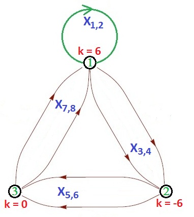
Figure 4: Quiver Diagram for Fano ${\cal B}_{3}$

There are $N_{T}=4$ terms in $W$ for the $G=3$ node quiver with $E=8$ matter fields. The quiver diagram can be constructed as shown in figure 4. Clearly, $N_{T}-E+G=-1$ and cannot admit tiling presentation. However, the abelian $W$ is non-zero. So, it must be possible to do the forward algorithm after deducing the quiver diagram with CS levels from the inverse algorithm.

To obtain the CS levels on the three nodes of the quiver, we need the matrix $P=K.T$:

$$P=\left(\begin{array}[]{ccccccc}3&0&1&0&0&0&1\\ 0&3&1&0&0&0&1\\ 3&0&0&1&0&0&1\\ 0&3&0&1&0&0&1\\ 0&0&4&0&6&0&1\\ 0&0&0&4&6&0&1\\ 0&0&4&0&0&6&1\\ 0&0&0&4&0&6&1\\ \end{array}\right)$$

Using the $Q_{D}$ charge (4.43) and the $P$-matrix elements, we can obtain the projected charge $\Delta$ of the matter fields and find the possible quiver as shown in figure 4 whose charge matrix $d$ is given below:

$$d=\left(\begin{array}[]{c|cccc}&X_{i}(i=1,2)&X_{i}(i=3,4)&X_{i}(i=5,6)&X_{i}(i=7,8)\\ \hline\cr a=1&0&1&0&-1\\ a=2&0&-1&1&0\\ a=3&0&0&-1&1\end{array}\right)~{},$$ (4.47)

The CS levels of the 3-nodes are

$$k_{1}=6,k_{2}=-6,k_{3}=0~{}.$$ (4.48)

4.4.1 Hilbert series evaluation for ${\cal B}_{3}$ Theory

The total charge matrix for the $B_{3}$ theory is given by:

$$Q=\left(\begin{array}[]{ccccccc}1&1&3&3&-1&-1&-6\\ 1&1&1&1&0&0&-4\\ 0&0&0&0&1&-1&0\end{array}\right)$$ (4.49)

The symmetry group for this theory is $SU(2)^{2}\times{U(1)}^{2}$. Here, we have 7 $p_{\alpha}$ fields. Let us denote the R-charge fugacity associated with the $p_{1}$, $p_{2}$ be $s_{1}$, with $p_{3}$, $p_{4}$ be $s_{2}$ and with $p_{5}$, ${\tilde{p}}_{5}$ to be $s_{3}$ and $s_{4}$ respectively. Since the R-charge of the internal point $p_{6}$ is 0, the corresponding fugacity is set to unity. Using the $Q$ matrix, the Hilbert series of the mesonic moduli space can be written as:

$$g^{mes}(s_{1},s_{2},s_{3},s_{4};{\cal B}_{3}) = \oint_{|z_{1}|=1}\left(\frac{\text{$dz_{1}$}}{2\pi\text{$\mathit{i}$$z_{1}$}}\right)\oint_{|b|=1}\left(\frac{\text{$db$}}{2\pi\text{$\mathit{i}$$b$}}\right)\oint_{|z_{2}|=1}\left(\frac{\text{$dz_{2}$}}{2\pi\text{$\mathit{i}$$z_{2}$}}\right)$$

$$\left\{\frac{1}{{\left(1-s_{1}z_{1}z_{2}\right)^{2}}\left(1-s_{2}z_{1}^{3}z_{2}\right)^{2}\left(1-s_{3}\frac{b}{z_{1}}\right)}\right.$$ (4.50)

$$\left.\frac{1}{\left(1-s_{4}\frac{1}{bz_{1}}\right)\left(1-\frac{1}{z_{1}^{6}z_{2}^{4}}\right)}\right\}$$

	$SU(2)_{1}$	$SU(2)_{2}$	$U(1)_{R}$	$U(1)_{B}$	$U(1)_{q}$	fugacity
$p_{1}$	1	0	0.164	0	1	$s_{1}x_{1}q$
$p_{2}$	-1	0	0.164	0	1	$s_{1}q/x_{1}$
$p_{3}$	0	1	0.782	0	-3	$s_{2}x_{2}/q^{3}$
$p_{4}$	0	-1	0.782	0	-3	$s_{2}/(x_{2}q^{3})$
$p_{5}$	0	0	0.039	1	0	$s_{3}b$
${\tilde{p}}_{5}$	0	0	0	-1	4	$s_{4}q^{4}/b$
$p_{6}$	0	0	0	0	0	$1$

Table 3: Various charges of perfect matchings under global symmetry of ${\cal B}_{3}$ theory. In this table, $s_{i}$ is the fugacity of R-charges, $x_{1}$ and $x_{2}$ are weights of two $SU(2)$ symmetries, $b$ and $q$ are fugacities of $U(1)_{B}$ and $U(1)_{q}$ symmetries respectively.

The Hilbert series for mesonic moduli space with the change of variables as $t_{1}=\left(s_{1}s_{2}^{1/3}\right)$ and $t_{2}=\left(s_{2}^{4/3}s_{3}s_{4}\right)$ turns out to be

$$g^{mes}(t_{1},t_{2};{\cal B}_{3}) = \frac{1}{\left(1-t_{2}^{3}\right)^{2}\left(1-t_{1}^{3}\right)^{3}}\left\{1+5t_{1}^{3}+9t_{1}^{2}t_{2}-3t_{1}^{5}t_{2}+8t_{1}t_{2}^{2}+t_{1}^{4}t_{2}^{2}-3t_{1}^{7}t_{2}^{2}\right.$$

$$~{}~{}\left.+3t_{2}^{3}-t_{1}^{3}t_{2}^{3}-8t_{1}^{6}t_{2}^{3}+3t_{1}^{2}t_{2}^{4}-9t_{1}^{5}t_{2}^{4}-5t_{1}^{4}t_{2}^{5}-t_{1}^{7}t_{2}^{5}\right\}~{}.$$ (4.51)

which is the form expected for toric CY 4-folds with two $U(1)$ symmetries. Suppose, $R_{1}$ and $R_{2}$ be the R-charges corresponding to the fugacities $t_{1}$ and $t_{2}$. That is, $t_{1}=e^{-\mu R_{1}}$ and $t_{2}=e^{-\mu R_{2}}$, where $\mu$ is the chemical potential for the R-charge. Similar to the volume minimisation done for earlier cases, we can find the value $\hat{R}_{1},\hat{R}_{2}$ which minimises the volume $V({\cal B}_{3})$. For the given $W$ (4.45), we find that $R_{1}+R_{2}=1/3$. Substituting this relation in the volume of ${\cal B}_{3}$ and minimising it, we get $R_{1}=\frac{1}{24}\left(-3+\sqrt{57}\right)=0.189$ and $R_{2}=\frac{1}{24}\left(11-\sqrt{57}\right)=0.144$. The R-charges of each $p_{\alpha}$ can be determined which we tabulate in Table 3.

5 Summary and open problems

In this paper, we have systematized inverse algorithm by understanding the pattern of the charge assignments $Q_{F},Q_{D}$ obtained for 14 Fano 3-folds from forward/tiling algorithm han8 . Particularly, we used the second Betti number, symmetry of the CY 4-folds to fix the number of rows of $Q_{D}$ charge matrix and the entries of both $Q_{F}$ and $Q_{D}$ matrix. Our ansatz in section 4.1, which states that the rank of the non-abelian symmetry of $Q_{F}$ is one higher than that of $Q_{D}$, indicates the multiplicity of which points in the toric data could be taken. Using the ansatz, we took a possible choice of $Q_{F},Q_{D}$ and performed the sequence of steps to obtain the quiver diagram, superpotential and the Chern-Simons levels.

The quivers for Fano ${\mbox{$\mathbb{P}$}}^{3},{\cal B}_{1},{\cal B}_{2}$ and ${\cal B}_{3}$ as shown in figures 1–4 with the appropriate $W$ constructed from $K$-matrix showed that they cannot admit tiling presentation. It appears that forward algorithm from the quiver data for ${\cal B}_{2}$ and ${\cal B}_{3}$ can be done to confirm the toric data.

Our charge assignments $Q_{F},Q_{D}$ for the four Fano 3-folds gives the expected form for the Hilbert series of the mesonic moduli space. So, we believe that our ansatz must be correct. Using the volume minimisation, we have tabulated the $R$-charge of the fields $p_{\alpha}$’s. We obtained the correct genus $g=33$ for ${\mbox{$\mathbb{P}$}}^{3}$ Fano. However, it is not clear why the genus computation for ${\cal B}_{2}$ is giving $g=33$ instead of $g=29$ han8 .

It will be interesting to do the higgsing approach tapo for CS quivers which does not admit tiling presentation. We hope to report on the higgsing procedure in a future publication. In ref. jpark , the tiling rules for $SO/Sp$ quivers corresponding to the orientifolds of the CY 3-folds were proposed. It is a challenging problem to generalise the tiling for orientifolds of the CY 4-folds forc corresponding to $SO/Sp$ CS quivers.

Acknowledgments: We would like to thank Tapobrata Sarkar and Prabwal Phukon for discussions during the initial stages of this project. P.R would like to thank the hospitality of Center for Quantum spacetime, Sogang University where this work was done during the sabbatical visit. This work was supported by the National Research Foundation of Korea(NRF) grant funded by the Korea government(MEST) through the Center for Quantum Spacetime(CQUeST) of Sogang University with grant number 2005-0049409.

References

- (1) J.Bagger and N.Lambert, “Modeling multiple M2’s,” Phys. Rev. D75, 045020 (2007) [arXiv:hep-th/0611108]. “Gauge symmetry and Supersymmetry of Multiple M2-Branes,” Phys. Rev. D77,065008 (2008) [arXiv:0711.0955[hep-th]]. “Comments on Multiple M2-branes,” JHEP0802, 105 (2008) [arXiv:0712.3738[hep-th]].
- (2) A.Gustavsson, “Algebraic structures on parallel M2-branes,” Nucl.Phys. B811, 66 (2009) [arXiv:0709.1260[hep-th]]. “Selfdual strings and loop space Nahm equations,” JHEP 0804, 083 (2008) [arXiv:0802.3456[hep-th]].
- (3) M.Van Raamsdonk, “Comments on the Bagger-Lambert theory and multiple M2-branes,” JHEP 0805, 105 (2008) [arXiv:0803.3803].
- (4) O.Aharony, O. Bergman, D.L. Jafferis and J. Maldacena, “N=6 superconformal Chern-Simons-matter theories, M2-branes and their gravity duals, ”JHEP 0810,091 (2008) [arXiv:0806.1218[hep-th]].
- (5) I.R.Klebanov and G.Torri, “M2-branes and AdS/CFT,” Int.J.Mod.Phys. A25 332 (2010) [arXiv:0909.1580[hep-th]].
- (6) D.Martelli and J. Sparks, “Moduli spaces of Chern-Simons quiver gauge theories and AdS4/CFT3,” Phys.Rev. D78, 126005 (2008) [arXiv:0808.0912[hep-th]].
- (7) B.Feng, A.Hanany and Y.H.He, “D-brane gauge theories from toric singularities and toric duality,” Nucl. Phys. B595, 165 (2001) [arXiv:hep-th/0003085].
- (8) A. Hanany and K.D. Kennaway, “Dimer models and toric diagrams,” [arXiv:hep-th/0503149].
- (9) S.Franco, A.Hanany, K.D. Kennaway,D.Vegh and B.Wecht, “Brane dimers and quiver gauge theories,” JHEP 0601, 096 (2006) [arXiv:hep-th/ 0504110].
- (10) A.Hanany and A.Zaffaroni, “Tilings, Chern-Simons Theories and M2 branes,” JHEP 0810, 111 (2008) [arXiv:0808.1244[hep-th]].
- (11) K.Ueda and M.Yamazaki, “Toric Calabi-Yau four-folds dual to Chern-Simons-matter theories,” JHEP 0812, 045 (2008) [arXiv:0808.3768[hep-th]].
- (12) A.Hanany, D.Vegh, A.Zaffaroni, “Brane Tilings and M2 branes,” JHEP 0903, 012 (2009) [arXiv:0809.1440].
- (13) S.Franco, A.Hanany, J.Park and D.Rodriguez-Gomez,“Towards M2-brane Theories for Generic Toric Singularities,”JHEP 0812, 110 (2008) [arXiv:0809.3237 [hep-th]].
- (14) A.Hanany and Y.H.He, “M2-branes and Quiver Chern-Simons: A Taxonomic Study,” arXiv:0811.4044[hep-th].
- (15) J.Davey, A.Hanany, N.Mekareeya and G.Torri, “Phases of M2-brane Theories,” JHEP 0906, 025 (2009) [arXiv:0903.3234[hep-th]].
- (16) J.Davey, A.Hanany, N.Mekareeya and G.Torri, “Higgsing M2-brane Theories,” arXiv:0908.4033[hep-th].
- (17) J.Davey, A.Hanany, N.Mekareeya and G.Torri, “M2-Branes and Fano 3-folds,” arXiv:1103.0553[hep-th].
- (18) P. Agarwal, P. Ramadevi, T. Sarkar, “A note on dimer models and D-brane gauge theories,” JHEP 0806 054 (2008) [arXiv:0804.1902].
- (19) Sangmin Lee,“Superconformal field theories from crystal lattices,” Phys.Rev.D75 101901 (2007)[arXiv:hep-th/0610204].
- (20) Sangmin Lee, Sungjay Lee and Jaemo Park, “Toric AdS4/CFT3 duals and M-theory Crystals,” JHEP 0705 004 (2007) [arXiv:hep-th/0702120].
- (21) Sebastian Franco, Amihay Hanany, Daniel Krefl, Jaemo Park, Angel M. Uranga and David Vegh, “ Dimers and Orientifolds”, JHEP 0709, 075 (2007) [arXiv:0707.0298[hep-th]].
- (22) Davide Forcella, Alberto Zaffaroni, “ N=1 Chern-Simons theories, orientifolds and Spin(7) cones”, JHEP 1005, 045 (2010) [arXiv:0911.2595[hep-th]].