1 Introduction

Application domains such as molecular biology and fMRI (e.g., Lu2005Hotelling, ; Goeman2007Analyzing, ; fMRI1, ; fMRI2, ) have stimulated considerable interest in two-sample hypothesis testing problems in the high-dimensional setting, where two samples of data $\{X_{1},\dots,X_{n_{1}}\}$ and $\{Y_{1},\dots,Y_{n_{2}}\}$ are subsets of $\mathbb{R}^{p}$, and $n_{1},n_{2}\ll p$. The problem of discriminating between two data-generating distributions becomes difficult in this context as the cumulative effect of variance in many variables can “explain away” the correct hypothesis. In transcriptomics, for instance, $p$ gene expression measures on the order of hundreds or thousands may be used to investigate differences between two biological conditions, and it is often difficult to obtain sample sizes $n_{1}$ and $n_{2}$ larger than several dozen in each condition. For problems such as these, classical methods may be ineffective, or not applicable at all. Likewise, there has been growing interest in developing testing procedures that are better suited to deal with the effects of dimension (e.g., BS96, ; SD2008, ; Srivastava2009, ; CQ2010, ; AUCopt, ).

A fundamental instance of the general two-sample problem is the two-sample test of means with Gaussian data. In this case, two independent sets of samples $\{X_{1},\dots,X_{n_{1}}\}$ and $\{Y_{1},\dots,Y_{n_{2}}\}\subset\mathbb{R}^{p}$ are generated in an i.i.d. manner from $p$-dimensional multivariate normal distributions $N(\mu_{1},\Sigma)$ and $N(\mu_{2},\Sigma)$ respectively, where the mean vectors $\mu_{1}$ and $\mu_{2}$, and positive-definite covariance matrix $\Sigma\succ 0$, are all fixed and unknown. The hypothesis testing problem of interest is

$${\bf{H}}_{0}:\mu_{1}=\mu_{2}\text{ \ versus \ }{\bf{H}}_{1}:\mu_{1}\neq\mu_{2}.$$ (1)

The most well-known test statistic for this problem is the Hotelling $T^{2}$ statistic, defined by

$$T^{2}:=\frac{n_{1}\,n_{2}}{n_{1}+n_{2}}\,(\bar{X}-\bar{Y})^{\top}\widehat{\Sigma}^{-1}\,(\bar{X}-\bar{Y}),$$ (2)

where $\bar{X}:=\frac{1}{n_{1}}\textstyle\sum_{j=1}^{n_{1}}X_{j}$ and $\bar{Y}:=\frac{1}{n_{2}}\textstyle\sum_{j=1}^{n_{2}}Y_{j}$ are the sample means, and $\widehat{\Sigma}$ is the pooled sample covariance matrix, given by $\widehat{\Sigma}:\,=\textstyle{\frac{1}{n}\,\textstyle\sum_{j=1}^{n_{1}}(X_{j}-\bar{X})(X_{j}-\bar{X})^{\top}+\ \frac{1}{n}\textstyle\sum_{j=1}^{n_{2}}(Y_{j}-\bar{Y})(Y_{j}-\bar{Y})^{\top}}$, where we define $n:=n_{1}+n_{2}-2$ for convenience.

When $p>n$, the matrix $\widehat{\Sigma}$ is singular, and the Hotelling test is not well-defined. Even when $p\leq n$, the Hotelling test is known to perform poorly if $p$ is nearly as large as $n$. This was shown in an important paper of Bai and Saranadasa (abbreviated BS) BS96 , who studied the performance of the Hotelling test under $(p,n)\to\infty$ with $p/n\to 1-\epsilon$, and showed that the asymptotic power of the test suffers for small values of $\epsilon>0$. Consequently, several improvements on the Hotelling test have been proposed in the high-dimensional setting in past years (e.g., BS96, ; SD2008, ; Srivastava2009, ; CQ2010, ).

Due to the well-known degradation of $\widehat{\Sigma}$ as an estimate of $\Sigma$ in high dimensions, the line of research on extensions of Hotelling test for problem (1) has focused on replacing $\widehat{\Sigma}$ in the definition of $T^{2}$ with other estimators of $\Sigma$. In the paper BS96 , BS proposed a test statistic based on the quantity $(\bar{X}-\bar{Y})^{\top}(\bar{X}-\bar{Y})$, which can be viewed as replacing $\widehat{\Sigma}$ with $I_{p\times p}$. It was shown by BS that this statistic achieves non-trivial asymptotic power whenever the ratio $p/n$ converges to a constant $c\in(0,\infty)$. This statistic was later refined by Chen and Qin CQ2010 (CQ for short) who showed that the same asymptotic power can be achieved without imposing any explicit restriction on the limit of $p/n$. Another direction was considered by Srivastava and Du SD2008 ; Srivastava2009 (SD for short), who proposed a test statistic based on $(\bar{X}-\bar{Y})^{\top}\widehat{D}^{-1}(\bar{X}-\bar{Y})$, where $\widehat{D}$ is the diagonal matrix associated with $\widehat{\Sigma}$, i.e. $\widehat{D}_{ii}=\widehat{\Sigma}_{ii}$. This choice ensures that $\widehat{D}$ is invertible for all dimensions $p$ with probability 1. Srivastava and Du demonstrated that their test has superior asymptotic power to the tests of BS and CQ under a certain parameter setting and local alternative when $n=\mathcal{O}(p)$. To the best of our knowledge, the procedures of CQ and SD represent the state-of-the-art among tests for problem (1) with a known asymptotic power function under the scaling $(p,n)\to\infty$.

In this paper, we propose a new testing procedure for problem (1) in the high-dimensional setting, which involves randomly projecting the $p$-dimensional samples into a space of lower dimension $k\leq\min\{n,p\}$, and then working with the Hotelling test in $\mathbb{R}^{k}$. Allowing $(p,n)\to\infty$, we derive an asymptotic power function for our test and show that it outperforms the tests of BS, CQ, and SD in terms of asymptotic relative efficiency under certain conditions. Our comparison results are valid with $p/n$ tending to a constant or infinity. Furthermore, whereas the mentioned testing procedures can only offer approximate level-$\alpha$ critical values, our procedure specifies exact level-$\alpha$ critical values for general multivariate normal data. Our test is also very easy to implement, and has a computational cost of order $\mathcal{O}(n^{2}p)$ operations when $k$ scales linearly with $n$, which is modest in the high-dimensional setting.

From a conceptual point of view, the procedure studied here is most distinct from past approaches in the way that covariance structure is incorporated into the test statistic. As stated above, the test statistics of BS, CQ, and SD are essentially based on versions of the Hotelling $T^{2}$ with diagonal estimators of $\Sigma$. Our analysis and simulations show that this limited estimation of $\Sigma$ sacrifices power when the data variables are correlated, or when most of the variance can be captured in a small number of variables. In this regard, our procedure is motivated by the idea that covariance structure may be used more effectively by testing with projected samples in a space of lower dimension. The use of projection-based test statistics has also been considered previously in Jacob et al. Jacob2010Gains and Clémençon et al. AUCopt .

The remainder of this paper is organized as follows. In Section 2, we discuss the intuition for our testing procedure, and then formally define the test statistic. Section 3 is devoted to a number of theoretical results about the performance of the test. Theorem 1 in Section 3.1 provides an asymptotic power function, and Theorems 2 and 3 in Sections 3.4 and 3.5 give sufficient conditions for achieving greater power than the tests of CQ and SD in the sense of asymptotic relative efficiency. In Sections 4.1 and 4.2, we use synthetic data to make performance comparisons with ROC and calibration curves against the mentioned tests, as well as some recent non-parametric procedures such as maximum mean discrepancy (MMD) (Gretton2007A, ), kernel Fisher discriminant analysis (KFDA) (Harchaoui2008Testing, ), and a test based on area-under-curve maximization, denoted TreeRank (AUCopt, ). These simulations show that our test outperforms competing tests in the parameter regimes anticipated by our theoretical results. Lastly, in Section 4.3 we study an example involving high-dimensional gene expression data, and demonstrate an advantage of our test in terms of its false positive rate when discriminating between different types of cancer.

Notation.

We use $\delta:=\mu_{1}-\mu_{2}$ to denote the shift vector between the distributions $N(\mu_{1},\Sigma)$ and $N(\mu_{2},\Sigma)$. For a positive-definite covariance matrix $\Sigma$, let $D_{\sigma}$ be the diagonal matrix obtained by setting the off-diagonal entries of $\Sigma$ to 0, and also define the associated correlation matrix $R:=D_{\sigma}^{-1/2}\Sigma D_{\sigma}^{-1/2}$. Let $z_{1-\alpha}$ denote the $1-\alpha$ quantile of the standard normal distribution, and let $\Phi$ be its cumulative distribution function. If $A$ is a matrix in $\mathbb{R}^{p\times p}$, let $\left|\kern-1.5pt\left|\kern-1.5pt\left|A\right|\kern-1.5pt\right|\kern-1.5pt\right|_{2}$ denote its spectral norm (maximum singular value), and define the Frobenius norm $\left|\kern-1.5pt\left|\kern-1.5pt\left|A\right|\kern-1.5pt\right|\kern-1.5pt\right|_{F}:=\sqrt{\sum_{i,j}A_{ij}^{2}}$. When all the eigenvalues of $A$ are real, we denote them by $\lambda_{\min}(A)=\lambda_{p}(A)\leq\cdots\leq\lambda_{1}(A)=\lambda_{\max}(A)$. If $A$ is positive-definite, we write $A\succ 0$, and $A\succeq 0$ if $A$ is positive semidefinite. We use the notation $f(n)\lesssim g(n)$ if there is some absolute constant $c\in(0,\infty)$ such that the inequality $f(n)\leq c\,n$ holds for all large $n$. If both $f(n)\lesssim g(n)$ and $g(n)\lesssim f(n)$ hold, then we write $f(n)\asymp g(n)$. The notation $f(n)=o(g(n))$ means $f(n)/g(n)\to 0$ as $n\to\infty$. For two random variables $X$ and $Y$, equality in distribution is written as $X\stackrel{{\scriptstyle d}}{{=}}Y$.

2 Random projection method

For the remainder of the paper, we retain the setup for the two-sample test of means (1) with Gaussian data given in Section 1. In particular, our procedure can be implemented with $p>n$ or $p\leq n$, as long as $k$ is chosen such that $k\leq\min\{n,p\}$. In Section 3.3, we demonstrate an optimality property of the choice $k=\lfloor n/2\rfloor$, which is valid in moderate or high-dimensions, i.e., $p\geq\lfloor n/2\rfloor$, and we restrict our attention to this case in Theorems 2 and 3.

2.1 Intuition for random projection method

At a high level, our method can be viewed as a two-step procedure. First, a single random projection $P_{k}^{\top}\in\mathbb{R}^{k\times p}$ is drawn, and is used to map the samples from the high-dimensional space $\mathbb{R}^{p}$ to a low-dimensional space $\mathbb{R}^{k}$. Second, the Hotelling $T^{2}$ test is applied to a new hypothesis testing problem, denoted ${\bf{H}}_{0,\text{proj}}$ versus ${\bf{H}}_{1,\text{proj}}$, in the projected space. A decision is then pulled back to the high-dimensional problem (1) by simply rejecting the original null hypothesis ${\bf{H}}_{0}$ whenever the Hotelling test rejects ${\bf{H}}_{0,\text{proj}}$ in the projected space.

To provide some intuition for our method, it is possible to consider the problem (1) in terms of a competition between the dimension $p$, and the “statistical distance” separating ${\bf{H}}_{0}$ and ${\bf{H}}_{1}$. On one hand, the accumulation of variance from a large number of variables makes it difficult to discriminate between the hypotheses, and thus, it is desirable to reduce the dimension of the data. On the other hand, methods for reducing dimension also tend to bring ${\bf{H}}_{0}$ and ${\bf{H}}_{1}$ “closer together,” making them harder to distinguish. Mindful of the fact that the Hotelling $T^{2}$ measures the separation of ${\bf{H}}_{0}$ and ${\bf{H}}_{1}$ in terms of the Kullback-Leibler divergence $D_{\text{KL}}(N(\mu_{1},\Sigma)\|N(\mu_{2},\Sigma))=\frac{1}{2}\delta^{\top}\Sigma^{-1}\delta$, with $\delta=\mu_{1}-\mu_{2}$, we see that the relevant statistical distance is driven by the length of $\delta$. Consequently, we seek to transform the data in a way that reduces dimension and preserves most of the length of $\delta$ upon passing to the transformed distributions. From this geometric point of view, it is natural to exploit the fact that random projections can simultaneously reduce dimension and approximately preserve length with high probability randProj .

In addition to reducing dimension in a way that tends to preserve statistical distance between ${\bf{H}}_{0}$ and ${\bf{H}}_{1}$, random projections have two other interesting properties with regard to the design of test statistics. Note that when the Hotelling test statistic is constructed from the projected samples in a space of dimension $k\leq\min\{n,p\}$, it is proportional to $[P_{k}^{\top}(\bar{X}-\bar{Y})]^{\top}(P_{k}^{\top}\widehat{\Sigma}P_{k})^{-1}[P_{k}^{\top}(\bar{X}-\bar{Y})]$. Thus, whereas the tests of BS, CQ, and SD replace $\widehat{\Sigma}$ in the definition of $T^{2}$ with a diagonal estimator, our procedure uses $P_{k}^{\top}\widehat{\Sigma}P_{k}$ as a $k\times k$ surrogate for $\widehat{\Sigma}$. The key advantage is that $P_{k}^{\top}\widehat{\Sigma}P_{k}$ retains some information about the off-diagonal entries of $\Sigma$. Another benefit offered by random projection concerns the robustness of critical values. In the classical setting where $p\leq n$, the critical values of the Hotelling test are exact in the presence of Gaussian data. It is also well-known from the projection pursuit literature that the empirical distribution of randomly projected data tends to be approximately Gaussian FreedmanDiaconis . Our procedure leverages these two facts by first “inducing Gaussianity” and then applying a test that has exact critical values for Gaussian data. Consequently, we expect that the critical values of our procedure may be accurate even when the $p$-dimensional data are not Gaussian, and this idea is illustrated by a simulation with data generated from a mixture model, as well as an example with real transcriptomic data in Section 4.3.

2.2 Formal testing procedure

For an integer $k\in\{1,\dots,\min\{n,p\}\}$, let $P_{k}^{\top}\in\mathbb{R}^{k\times p}$ denote a random matrix with i.i.d. $N(0,1)$ entries, drawn independently of the data. Conditioning on a given draw of $P_{k}^{\top}$, the projected samples $\{P_{k}^{\top}X_{1},\dots,P_{k}^{\top}X_{n_{1}}\}$ and $\{P_{k}^{\top}Y_{1},\dots,P_{k}^{\top}Y_{n_{2}}\}$ are distributed i.i.d. according to $N(P_{k}^{\top}\mu_{i},P_{k}^{\top}\Sigma P_{k})$ respectively, with $i=1,2$. Since the projected data are Gaussian and lie in a space of dimension no larger than $n$, it is natural to consider applying the Hotelling test to the following two-sample problem in the projected space $\mathbb{R}^{k}$:

$${\bf{H}}_{0,\text{proj}}:P_{k}^{\top}\mu_{1}=P_{k}^{\top}\mu_{2}\text{ \ versus \ }{\bf{H}}_{1,\text{proj}}:P_{k}^{\top}\mu_{1}\neq P_{k}^{\top}\mu_{2}.$$ (3)

For this projected problem, the Hotelling test statistic takes the form

$$T_{k}^{2}:=\frac{n_{1}n_{2}}{n_{1}+n_{2}}[P_{k}^{\top}(\bar{X}-\bar{Y})]^{\top}(P_{k}^{\top}\widehat{\Sigma}P_{k})^{-1}[P_{k}^{\top}(\bar{X}-\bar{Y})],$$

where $\bar{X}$, $\bar{Y}$, and $\widehat{\Sigma}$ are as stated in the introduction. Note that $P_{k}^{\top}\widehat{\Sigma}P_{k}$ is invertible with probability 1 when $P_{k}^{\top}$ has i.i.d. $N(0,1)$ entries, which ensures that $T_{k}^{2}$ is well-defined, even when $p>n$.

When conditioned on a draw of $P_{k}^{\top}$, the $T_{k}^{2}$ statistic has an $\frac{k\,n}{n-k+1}F_{k,n-k+1}$ distribution under ${\bf{H}}_{0,\text{proj}}$, since it is an instance of the Hotelling test statistic (Muirhead, , p. 216). Inspection of the formula for $T_{k}^{2}$ also shows that its distribution is the same under both ${\bf{H}}_{0}$ and ${\bf{H}}_{0,\text{proj}}$. Consequently, if we let $t_{\alpha}:=\frac{k\,n}{n-k+1}F^{1-\alpha}_{k,n-k+1}$, where $F^{1-\alpha}_{k,n-k+1}$ is the $1-\alpha$ quantile of the $F_{k,n-k+1}$ distribution, then the condition $T_{k}^{2}\geq t_{\alpha}$ is a level-$\alpha$ decision rule for rejecting the null hypothesis in both the projected problem (3) and the original problem (1). Accordingly, we define this as the condition for rejecting ${\bf{H}}_{0}$ at level $\alpha$ in our procedure for (1). We summarize the implementation of our procedure below.

Implementation of random projection-based test at level $\alpha$ for problem (1).

$$\boxed{\begin{split}&\text{1. Generate a single random matrix $P_{k}^{\top}\in\mathbb{R}^{k\times p}$ with i.i.d. $N(0,1)$ entries.}\\ &\text{2. Compute $T_{k}^{2}$, using $P_{k}^{\top}$ and the two sets of samples.}\\ &\text{3. If $T_{k}^{2}\geq t_{\alpha}$, reject ${\bf{H}}_{0}$; otherwise accept ${\bf{H}}_{0}$.}\\ \end{split}} \star$$ ()

3 Main results and their consequences

This section is devoted to the statement and discussion of our main theoretical results, including an asymptotic power function for our test (Theorem 1), and comparisons of asymptotic relative efficiency with state-of-the-art tests proposed in past work (Theorems 2 and 3).

3.1 Asymptotic power function

Our first main result characterizes the asymptotic power of the $T_{k}^{2}$ test statistic in the high-dimensional setting. As is standard in high-dimensional asymptotics, we consider a sequence of hypothesis testing problems indexed by $n$, allowing the dimension $p$, sample sizes $n_{1}$ and $n_{2}$, mean vectors $\mu_{1}$ and $\mu_{2}$ and covariance matrix $\Sigma$ to implicitly vary as functions of $n$, with $n$ tending to infinity. We also make another type of asymptotic assumption, known as a local alternative, which is commonplace in hypothesis testing (e.g., see van der Vaart (vdv, , §14.1)). The idea lying behind a local alternative assumption is that if the difficulty of discriminating between ${\bf{H}}_{0}$ and ${\bf{H}}_{1}$ is “held fixed” with respect to $n$, then it is often the case that most testing procedures have power tending to 1 under ${\bf{H}}_{1}$ as $n\to\infty$. In such a situation, it is not possible to tell if one test has greater asymptotic power than another. Consequently, it is standard to derive asymptotic power results under the extra condition that ${\bf{H}}_{0}$ and ${\bf{H}}_{1}$ become harder to distinguish as $n$ grows. This theoretical device aids in identifying the conditions under which one test is more powerful than another. The following local alternative (A0), and balancing assumption (A1), are the same as those used by Bai and Saranadasa BS96 to study the asymptotic power of the classical Hotelling test under $(n,p)\to\infty$. In particular, the local alternative (A0) means that the Kullback-Leibler divergence between the $p$-dimensional sampling distributions, $D_{\text{KL}}(N(\mu_{1},\Sigma)\,\|\,N(\mu_{2},\Sigma))=\frac{1}{2}\delta^{\top}\Sigma^{-1}\delta$, tends to $0$ as $n\to\infty$.

(A0) (Local alternative.) The shift vector and covariance matrix satisfy $\delta^{\top}\Sigma^{-1}\delta=o(1)$.

(A1) There is a constant $b\in(0,1)$ such that $n_{1}/n\to b$.

(A2) There is a constant $y\in(0,1)$ such that $k/n\to y$.

To set some notation for our asymptotic power result in Theorem 1, let $\theta:=(\delta,\Sigma)$ be an ordered pair containing the relevant parameters for problem (1), and define $\Delta_{k}^{2}$ as twice the Kullback-Leibler divergence between the projected sampling distributions,

$$\Delta_{k}^{2} :=2\,D_{\text{KL}}\left(N(P_{k}^{\top}\mu_{1},P_{k}^{\top}\Sigma P_{k})\,\big{\|}\,N(P_{k}^{\top}\mu_{2},P_{k}^{\top}\Sigma P_{k})\right)\;=\;\delta^{\top}P_{k}(P_{k}^{\top}\Sigma P_{k})^{-1}P_{k}^{\top}\delta.$$ (4)

When interpreting the statement of Theorem 1 below, it is important to notice that each time the procedure ($\star$ ‣ 2.2) is implemented, a draw of $P_{k}^{\top}$ induces a new test statistic $T_{k}^{2}$. Making this dependence on $P_{k}^{\top}$ explicit, let $\beta(\theta;P_{k}^{\top})$ denote the exact (non-asymptotic) power function of the $T_{k}^{2}$ statistic at level $\alpha$ for problem (1), conditioned on a given draw of $P_{k}^{\top}$, as in procedure ($\star$).

Theorem 1.

Assume conditions (A0), (A1), and (A2). Then, for almost all sequences of projections $P_{k}^{\top}$, the power function $\beta(\theta;P_{k}^{\top})$ satisfies

$$\beta(\theta;P_{k}^{\top})-\Phi\left(-z_{1-\alpha}+b(1-b)\sqrt{\frac{1-y}{2y}}\,\Delta_{k}^{2}\,\sqrt{n}\,\right) \to 0\quad\mbox{ as $n\to\infty$.}$$ (5)

Remarks. Notice that if $\Delta_{k}^{2}=0$ (e.g. under ${\bf{H}}_{0}$), then $\Phi(-z_{1-\alpha}+0)=\alpha$, which corresponds to blind guessing at level $\alpha$. Consequently, the second term $b(1-b)\sqrt{\frac{1-y}{2y}}\,\Delta_{k}^{2}\,\sqrt{n}$ determines the advantage of our procedure over blind guessing. Since $\Delta_{k}^{2}$ is twice the KL-divergence between the projected sampling distributions, these observations conform to the intuition from Section 2 that the KL-divergence measures the discrepancy between ${\bf{H}}_{0}$ and ${\bf{H}}_{1}$.

Proof of Theorem 1. Let $\beta_{\text{H}}(\theta;P_{k}^{\top})$ denote the exact power of the Hotelling test for the projected problem (3) at level $\alpha$. As a preliminary step, we verify that

$$\beta(\theta;P_{k}^{\top})=\beta_{\text{H}}(\theta;P_{k}^{\top}),$$ (6)

for almost all $P_{k}^{\top}$. To see this, first recall from Section 2 that the condition $T_{k}^{2}\geq t_{\alpha}$ is a level-$\alpha$ rejection criterion in both the procedure ($\star$ ‣ 2.2) for the original problem (1), and the Hotelling test for the projected problem (3). Next, note that if ${\bf{H}}_{1}:\delta\neq 0$ holds, then ${\bf{H}}_{1,\text{proj}}:P_{k}^{\top}\delta\neq 0$ holds with probability 1, since $P_{k}^{\top}\delta$ is distributed as $N(0,\|\delta\|_{2}^{2}\,I_{k\times k})$. Consequently, for almost all $P_{k}^{\top}$, the level-$\alpha$ decision rule $T_{k}^{2}\geq t_{\alpha}$ has the same power against the alternative in both the original and the projected problems, which verifies (6). This establishes a technical link that allows results on the power of the classical Hotelling test to be transferred to the high-dimensional problem (1).

In order to complete the proof, we use a result of Bai and Saranadasa (BS96, , Theorem 2.1), which asserts that if $\Delta_{k}^{2}=o(1)$ holds for a fixed sequence of projections $P_{k}^{\top}$, and assumptions (A1) and (A2) hold, then $\beta_{\text{H}}(\theta;P_{k}^{\top})$ satisifes

$$\beta_{\text{H}}(\theta;P_{k}^{\top})-\Phi\left(-z_{1-\alpha}+b(1-b)\sqrt{\frac{1-y}{2y}}\,\Delta_{k}^{2}\,\sqrt{n}\,\right)\to 0\text{ \ as \ }n\to\infty.$$ (7)

To ensure $\Delta_{k}^{2}=o(1)$, we appeal to a deterministic matrix inequality that follows from the proof of Lemma 3 in Jacob et al. Jacob2010Gains . Namely, for any full rank matrix $M^{\top}\in\mathbb{R}^{k\times p}$, and any $\delta\in\mathbb{R}^{p}$,

$$\delta^{\top}M(M^{\top}\Sigma M)^{-1}M^{\top}\delta\,\leq\,\delta^{\top}\Sigma^{-1}\delta.$$

Since $P_{k}^{\top}$ is full rank with probability 1, we see that $\Delta_{k}^{2}\leq\delta^{\top}\Sigma^{-1}\delta\to 0$ for almost all sequences of $P_{k}^{\top}$ under the local alternative (A0), as needed. Thus, the proof of Theorem 1 is completed by combining equation (6) with the limit (7).∎

3.2 Asymptotic relative efficiency (ARE)

Having derived an asymptotic power function in Theorem 1, we are now in position to provide a detailed comparison with the tests of CQ CQ2010 and SD SD2008 ; Srivastava2009 . We denote the asymptotic power function of our level-$\alpha$ random projection-based test (RP) by

$$\beta_{\text{RP}}(\theta;P_{k}^{\top}):=\Phi\left(-z_{1-\alpha}+b(1-b)\sqrt{\frac{1-y}{2y}}\,\Delta_{k}^{2}\,\sqrt{n}\,\right),$$ (8)

where we recall $\theta:=(\delta,\Sigma)$. The asymptotic power functions for the level-$\alpha$ testing procedures of CQ CQ2010 and SD SD2008 ; Srivastava2009 are given by

$$\beta_{\text{CQ}}(\theta) :=\ \Phi\left(-z_{1-\alpha}+{\frac{b(1-b)}{\sqrt{2}}\,\frac{\|\delta\|_{2}^{2}\,n}{\left|\kern-1.5pt\left|\kern-1.5pt\left|\Sigma\right|\kern-1.5pt\right|\kern-1.5pt\right|_{F}}}\right),\quad\mbox{and}$$ (9a)

$$\beta_{\text{SD}}(\theta) :=\ \Phi\left(-z_{1-\alpha}+{\frac{b(1-b)}{\sqrt{2}}\,\frac{\delta^{\top}D_{\sigma}^{-1}\delta\,n}{\left|\kern-1.5pt\left|\kern-1.5pt\left|R\right|\kern-1.5pt\right|\kern-1.5pt\right|_{F}}}\right),$$ (9b)

where $D_{\sigma}$ denotes the matrix formed by setting the off-diagonal entries of $\Sigma$ to 0, and $R$ denotes the correlation matrix associated to $\Sigma$. The functions $\beta_{\text{CQ}}$ and $\beta_{\text{SD}}$ are derived under local alternatives and asymptotic assumptions that are similar to the ones used here to obtain $\beta_{\text{RP}}$. In particular, all three functions can be obtained allowing $p/n$ to tend to an arbitrary positive constant, or to infinity.

A standard method of comparing asymptotic power functions is through the concept of asymptotic relative efficiency, or ARE for short (e.g., see van der Vaart (vdv, , ch. 14-15)). Since the term added to $-z_{1-\alpha}$ inside the $\Phi$ function is what controls power, the relative efficiency of tests is defined by the ratio of such terms. More explicitly, we define

$$\text{ARE}\left(\beta_{\text{CQ}};\beta_{\text{RP}}\right) :=\Big{(}\textstyle{{\frac{\|\delta\|_{2}^{2}\,n}{\left|\kern-1.5pt\left|\kern-1.5pt\left|\Sigma\right|\kern-1.5pt\right|\kern-1.5pt\right|_{F}}}\Big{/}\sqrt{\frac{1-y}{y}}\,\Delta_{k}^{2}\,\sqrt{n}}\Big{)}^{2},\quad\mbox{and}$$ (10a)

$$\text{ARE}\left(\beta_{\text{SD}};\beta_{\text{RP}}\right) :=\Big{(}\textstyle{{\frac{\delta^{\top}D_{\sigma}^{-1}\delta\,n}{\left|\kern-1.5pt\left|\kern-1.5pt\left|R\right|\kern-1.5pt\right|\kern-1.5pt\right|_{F}}}\Big{/}\sqrt{\frac{1-y}{y}}\,\Delta_{k}^{2}\,\sqrt{n}}\Big{)}^{2}.$$ (10b)

Whenever the ARE is less than 1, our procedure is considered to have greater asymptotic power than the competing test—with our advantage being greater for smaller values of the ARE. Consequently, we seek sufficient conditions in Theorems 2 and 3 below for ensuring that the ARE is small.

In classical analyses of asymptotic relative efficiency, the ARE is usually a deterministic quantity that does not depend on $n$. However, in the current context, our use of high-dimensional asymptotics, as well as a randomly constructed test statistic, lead to an ARE that varies with $n$ and is random. (In other words, the ARE specifies a sequence of random variables indexed by $n$.) Moreover, the dependence of the ARE on $\Delta_{k}^{2}$ implies that the ARE is affected by the orientation of the shift vector $\delta$. To consider an average-case scenario, where no single orientation of $\delta$ is of particular importance, we place a prior on $\delta$, and assume that it follows a spherical distribution with $\mathbb{P}(\delta=0)=0$. This implies that the orientation $\delta/\|\delta\|_{2}$ of the shift follows the uniform (Haar) distribution on the unit sphere. We emphasize that our procedure ($\star$ ‣ 2.2) does not rely on this choice of prior, and that it is only a device for making an average-case comparison against CQ and SD in Theorems 2 and 3. Lastly, we point out that a similar assumption was considered by Srivastava and Du SD2008 , who let $\delta$ be a deterministic vector with all coordinates equal to the same value, in order to compare with the results of BS BS96 .

To be clear about the meaning of Proposition 1 and Theorems 2 and 3 below, we henceforth regard the ARE as a function of two random objects, $P_{k}^{\top}$ and $\delta$, and our probability statements are made with this understanding. We complete the preparation for our comparison theorems by stating Proposition 1 and several limiting assumptions with $n\to\infty$.

(A3) The shift $\delta$ has a spherical distribution with $\mathbb{P}(\delta=0)=0$, and is independent of $P_{k}^{\top}$.

(A4) There is a constant $a\in[0,1)$ such that $k/p\to a$.

(A5) Assume $\frac{1}{\sqrt{k}}\,\frac{\operatorname{tr}(\Sigma)}{p\,\lambda_{\text{min}}(\Sigma)}=o(1)$.

(A6) Assume $\frac{\left|\kern-1.5pt\left|\kern-1.5pt\left|D_{\sigma}^{-1}\right|\kern-1.5pt\right|\kern-1.5pt\right|_{2}}{\operatorname{tr}(D_{\sigma}^{-1})}=o(1)$.

As can be seen from the formulas for $\beta_{\text{RP}}$ and the ARE, the performance of the $T_{k}^{2}$ statistic is determined by the random quantity $\Delta_{k}^{2}$. The following proposition provides interpretable upper and lower bounds on $\Delta_{k}^{2}$ that hold with high-probability. This proposition is the main technical tool needed for our comparison results in Theorems 2 and 3. A proof is given in Appendix B.

Proposition 1.

Under conditions (A3), (A4), and (A5), let $c$ be any positive constant strictly less than $(1-\sqrt{a})^{2}$, and let $C$ be any constant strictly greater than $\frac{(1+\sqrt{a})^{2}}{(1-\sqrt{a})^{2}}$. Then, as $n\to\infty$, we have

$$\mathbb{P}\left(\frac{\Delta_{k}^{2}}{\|\delta\|_{2}^{2}}\geq\frac{c\,k}{\operatorname{tr}(\Sigma)}\right) \to 1,\quad\mbox{and}$$ (11a)

$$\vskip 12.0pt plus 4.0pt minus 4.0pt\mathbb{P}\left(\frac{\Delta_{k}^{2}}{\|\delta\|_{2}^{2}}\leq\frac{C\,k}{p\,\lambda_{\min}(\Sigma)}\right) \to 1.$$ (11b)

Remarks. Although we have presented upper and lower bounds in an asymptotic manner, our proof specifies non-asymptotic bounds on $\Delta_{k}^{2}/\|\delta\|_{2}^{2}$. Due to the fact that Proposition 1 is a tool for making asymptotic comparisons of power in Theorems 2 and 3, it is sufficient and simpler to state the bounds in this asymptotic form. Note that if the condition $\operatorname{tr}(\Sigma)\asymp p\,\lambda_{\min}(\Sigma)$ holds, then Proposition 1 is sharp in the sense the upper and lower bounds (11a) and (11b) match up to constants.

3.3 Choice of projection dimension $k=\lfloor n/2\rfloor$

We now demonstrate an optimality property of the choice of projected dimension $k=\lfloor n/2\rfloor$. Note that this choice implicitly assumes $p\geq\lfloor n/2\rfloor$, but this does not affect the applicability of procedure ($\star$ ‣ 2.2) in moderate or high-dimensions. Letting $k/n\to y\in(0,1)$ as in assumption (A2), recall that the asymptotic power function from Theorem 1 is

$$\Phi\left(-z_{1-\alpha}+b(1-b)\sqrt{\frac{1-y}{2y}}\,\Delta_{k}^{2}\,\sqrt{n}\,\right).$$

Since Proposition 1 indicates that $\Delta_{k}^{2}$ scales linearly in $k$ up to random fluctuations, we see that formally replacing $k$ with $y\,n$ leads to maximizing the function $f(y):=\sqrt{\frac{1-y}{2y}}\,y$. The fact that $f$ is maximized at $y=1/2$ suggests that in certain cases, $k=\lfloor n/2\rfloor$ may be asymptotically optimal in a suitable sense. Considering a simple case where $\Sigma=\sigma^{2}\,I_{p\times p}$ for some absolute constant $\sigma^{2}>0$, it can be shown that under assumptions (A2), (A3), and integrability of $\|\delta\|_{2}^{2}$,

$$\frac{p}{n}\,\frac{\mathbb{E}(\Delta_{k}^{2})}{\mathbb{E}(\|\delta\|_{2}^{2})}\to y/\sigma^{2},$$ (12)

for all  $y\in(0,1)$, as $n\to\infty$. The following proposition is an immediate extension of this observation, and shows that $k=\lfloor n/2\rfloor$ is optimal in a precise sense for parameter settings that include $\Sigma=\sigma^{2}\,I_{p\times p}$ as a special case. Namely, as $n\to\infty$, the quantity $\sqrt{\frac{1-y}{2y}}\,\Delta_{k}^{2}$ is largest on average for $k=\lfloor n/2\rfloor$ among all choices of $k$, under the conditions stated below.

Proposition 2.

In addition to assumptions (A2) and (A3), suppose that $\|\delta\|_{2}^{2}$ is integrable. Also assume that for some absolute constant $\sigma^{2}>0$, the limit (12) holds for any $y\in(0,1)$. Let  $y^{*}=1/2$, and $k^{*}=\lfloor n/2\rfloor$. Then, for any  $y\in(0,1)$,

$$\lim_{n\to\infty}\frac{\sqrt{\frac{1-y^{*}}{2y^{*}}}\,\mathbb{E}(\Delta_{k^{*}}^{2})}{\sqrt{\frac{1-y}{2y}}\,\mathbb{E}(\Delta_{k}^{2})}=\frac{1}{2\sqrt{y(1-y)}}\geq 1.$$ (13)

(a) Setting (1)

(b) Setting (2)

Figure 1: Setting (1) corresponds to $\Sigma=\sigma^{2}\,I_{p\times p}$ with $\sigma^{2}=50$, and Setting (2) involves a covariance matrix $\Sigma$ with randomly selected eigenvectors and a rapidly decaying spectrum. The ROC curves indicate that $k=\lfloor n/2\rfloor$ is optimal, or nearly optimal, among the five choices of $y$ in the two settings.

Remarks. The ROC curves in Figure 1 illustrate several choices of projection dimension, with $k=\lfloor yn\rfloor$ and $y=0.1,\,0.3,\,0.5,\,0.7,\,0.9$, under two different parameter settings. In Setting (1), $\Sigma=\sigma^{2}\,I_{p\times p}$ with $\sigma^{2}=50$, and in Setting (2), the matrix $\Sigma$ was constructed with a rapidly decaying spectrum, and a matrix of eigenvectors drawn from the uniform (Haar) distribution on the orthogonal group, as in panel (d) of Figure 3 (see Section 4.1 for additional details). The curves in both settings were generated by sampling $n_{1}=n_{2}=50$ data at points from each of the distributions $N(\mu_{1},\Sigma)$ and $N(\mu_{2},\Sigma)$ in $p=200$ dimensions, and repeating the process 2000 times under both ${\bf{H}}_{0}$ and ${\bf{H}}_{1}$. For the experiments under ${\bf{H}}_{1}$, the shift $\delta$ was drawn uniformly from a sphere of radius 3 for Setting (1), and radius 1 for Setting (2)—in accordance with assumption (A3) in Proposition 2. Note that $k=\lfloor n/2\rfloor$ gives the best ROC curve for Setting (1) in Figure 1, which agrees with the fact that $\Sigma=\sigma^{2}\,I_{p\times p}$ satisfies the conditions of Proposition 2. In Setting (2), we see that the choice $k=\lfloor n/2\rfloor$ is not far from optimal, even when $\Sigma$ is very different from $\sigma^{2}I_{p\times p}$.

3.4 Power comparison with CQ

The next result provides a sufficient condition for the $T_{k}^{2}$ statistic to be asymptotically more powerful than the test of CQ. A proof is given at the end of this section (3.4).

Theorem 2.

Under the conditions of Proposition 1, suppose that we use a projection dimension $k=\lfloor n/2\rfloor$, where we assume $p\geq\lfloor n/2\rfloor$. Fix a number $\epsilon_{1}>0$, and let $c_{1}(\epsilon_{1})$ be any constant strictly greater than $\frac{4}{\epsilon_{1}(1-\sqrt{a})^{4}}$. If the condition

$$n\geq c_{1}(\epsilon_{1})\,\frac{\operatorname{tr}(\Sigma)^{2}}{\left|\kern-1.5pt\left|\kern-1.5pt\left|\Sigma\right|\kern-1.5pt\right|\kern-1.5pt\right|_{F}^{2}},$$ (14)

holds for all large $n$, then $\mathbb{P}\left[{\text{ARE}}\left(\beta_{\text{CQ}};\beta_{\text{RP}}\right)\leq\epsilon_{1}\right]\to 1$ as $n\to\infty$.

Remarks. The case of $\epsilon_{1}=1$ serves as the reference for equal asymptotic performance, with values $\epsilon_{1}<1$ corresponding to the $T_{k}^{2}$ statistic being asymptotically more powerful than the test of CQ. To interpret the result, note that Jensen’s inequality implies that the ratio $\operatorname{tr}(\Sigma)^{2}/\left|\kern-1.5pt\left|\kern-1.5pt\left|\Sigma\right|\kern-1.5pt\right|\kern-1.5pt\right|_{F}^{2}$ lies between $1$ and $p$, for any choice of $\Sigma$. As such, it is reasonable to interpret this ratio as a measure of the effective dimension of the covariance structure. The message of Theorem 2 is that as long as the sample size $n$ grows faster than the effective dimension, then our projection-based test is asymptotically superior to the test of CQ.

The ratio $\operatorname{tr}(\Sigma)^{2}/\left|\kern-1.5pt\left|\kern-1.5pt\left|\Sigma\right|\kern-1.5pt\right|\kern-1.5pt\right|_{F}^{2}$ can also be viewed as measuring the decay rate of the spectrum of $\Sigma$, with the condition $\operatorname{tr}(\Sigma)^{2}\big{/}\left|\kern-1.5pt\left|\kern-1.5pt\left|\Sigma\right|\kern-1.5pt\right|\kern-1.5pt\right|_{F}^{2}\ll p$ indicating rapid decay. This condition means that the data has low variance in “most” directions in $\mathbb{R}^{p}$, and so projecting onto a random set of $k$ directions will likely map the data into a low-variance subspace in which it is harder for chance variation to explain away the correct hypothesis, thereby resulting in greater power.

Example 1.

One instance of spectrum decay occurs when the top $s$ eigenvalues of $\Sigma$ contain most of the mass in the spectrum. When $\Sigma$ is diagonal, this has the interpretation that $s$ variables capture most of the total variance in the data. For simplicity, assume $\lambda_{1}=\cdots=\lambda_{s}>1$ and $\lambda_{s+1}=\cdots=\lambda_{p}=1$, which is similar to the spiked covariance model introduced by Johnstone Johnstone . If the top $s$ eigenvalues contain half of the total mass of the spectrum, then $s\,\lambda_{1}=(p-s)$, and a simple calculation shows that

$$\begin{split}\frac{\operatorname{tr}(\Sigma)^{2}}{\left|\kern-1.5pt\left|\kern-1.5pt\left|\Sigma\right|\kern-1.5pt\right|\kern-1.5pt\right|_{F}^{2}}&=\frac{4\,\lambda_{1}^{2}}{\lambda_{1}^{2}+\lambda_{1}}\,s\leq 4s.\\ \end{split}$$ (15)

This again illustrates the idea that condition (14) is satisfied as long as $n$ grows at a faster rate than the effective number of variables $s$. It is straightforward to check that this example satisfies assumption (A5) of Theorem 2 when, for instance, $\lambda_{1}=o(\sqrt{k})$.

Example 2.

Another example of spectrum decay can be specified by $\lambda_{i}(\Sigma)\propto i^{-\nu}$, for some absolute proportionality constant, a rate parameter $\nu\in(0,\infty)$, and $i=1,\dots,p$. This type of decay arises in connection with the Fourier coefficients of functions in Sobolev ellipsoids (Was06, , §7.2). Noting that $\operatorname{tr}(\Sigma)\asymp\int_{1}^{p}x^{-\nu}dx$ and $\left|\kern-1.5pt\left|\kern-1.5pt\left|\Sigma\right|\kern-1.5pt\right|\kern-1.5pt\right|_{F}^{2}\asymp\int_{1}^{p}x^{-2\nu}dx,$ direct computation of the integrals shows that

$$\frac{\operatorname{tr}(\Sigma)^{2}}{\left|\kern-1.5pt\left|\kern-1.5pt\left|\Sigma\right|\kern-1.5pt\right|\kern-1.5pt\right|_{F}^{2}}\asymp\begin{cases}1&\text{ if }\nu>1\\ \log^{2}p&\text{ if }\nu=1\\ p^{2(1-\nu)}&\text{ if }\nu\in(\frac{1}{2},1)\\ p/\log p&\text{ if }\nu=\frac{1}{2}\\ p&\text{ if }\nu\in(0,\frac{1}{2})\\ \end{cases}.$$

Thus, a decay rate given by $\nu\geq 1$ is easily sufficient for condition (14) to hold unless the dimension grows exponentially with $n$. On the other hand, decay rates associated to $\nu\leq 1/2$ are too slow for condition (14) to hold when $n\ll p$, and rates corresponding to $\nu\in(\frac{1}{2},1)$ lead to a more nuanced competition between $p$ and $n$. Assumption (A5) of Theorem 2 holds for all $\nu\in(0,1)$, but when $\nu=1$ or $\nu>1$, the dimension $p$ must satisfy the extra conditions $\log p=o(\sqrt{k})$ or $p^{\nu-1}=o(\sqrt{k})$ respectively.

The proof of Theorem 2  is a direct application of Proposition 1.

Proof of Theorem 2. Recalling $\text{ARE}\left(\beta_{\text{CQ}};\beta_{\text{RP}}\right)=\Big{(}{\frac{n\|\delta\|_{2}^{2}}{\left|\kern-1.5pt\left|\kern-1.5pt\left|\Sigma\right|\kern-1.5pt\right|\kern-1.5pt\right|_{F}}}\Big{/}\sqrt{n}\Delta_{k}^{2}\Big{)}^{2}$, with $k=\lfloor n/2\rfloor$ and $y=1/2$, the event of interest,

$$\text{ARE}\left(\beta_{\text{CQ}};\beta_{\text{RP}}\right)\leq\epsilon_{1},$$ (16)

is the same as

$$\frac{n}{\left|\kern-1.5pt\left|\kern-1.5pt\left|\Sigma\right|\kern-1.5pt\right|\kern-1.5pt\right|_{F}^{2}}\frac{1}{\epsilon_{1}}\leq\left(\frac{\Delta_{k}^{2}}{\|\delta\|_{2}^{2}}\right)^{2}.$$

By Proposition 1, we know that for any positive constant $c$ strictly less than $(1-\sqrt{a})^{2}$, the probability of the event

$$\frac{c\,k}{\operatorname{tr}(\Sigma)}\leq\frac{\Delta_{k}^{2}}{\|\delta\|_{2}^{2}}.$$ (17)

tends to 1 as $n\to\infty$. Consequently, as long as the inequality

$$\frac{n}{\left|\kern-1.5pt\left|\kern-1.5pt\left|\Sigma\right|\kern-1.5pt\right|\kern-1.5pt\right|_{F}^{2}}\frac{1}{\epsilon_{1}}\leq\left(\frac{c\,k}{\operatorname{tr}(\Sigma)}\right)^{2},$$ (18)

holds for all large $n$, then the event (16) of interest will also have probability tending to 1. Replacing $k$ with $\frac{n}{2}\cdot[1-o(1)]$, the last condition is the same as

$$n\geq\frac{\operatorname{tr}(\Sigma)^{2}}{\left|\kern-1.5pt\left|\kern-1.5pt\left|\Sigma\right|\kern-1.5pt\right|\kern-1.5pt\right|_{F}^{2}}\cdot\frac{4}{\epsilon_{1}\,c^{2}\,[1-o(1)]^{2}}.$$ (19)

Thus, for a given choice of $c_{1}(\epsilon_{1})$ in the statement of the theorem, it is possible to choose a positive $c<(1-\sqrt{a})^{2}$ so that inequality (18) is implied by the claimed sufficient condition (14) for all large $n$.∎

3.5 Power comparison with SD

We now give a sufficient condition for our procedure to be asymptotically more powerful than SD.

Theorem 3.

In addition to the conditions of Theorem 2, assume that (A6) holds. Fix a number $\epsilon_{1}>0$, and let $c_{1}(\epsilon_{1})$ be any constant strictly greater than $\frac{4}{\epsilon_{1}(1-\sqrt{a})^{4}}$. If the condition

$$n\geq c_{1}(\epsilon_{1})\left(\frac{\operatorname{tr}(\Sigma)}{p}\right)^{2}\left(\frac{\operatorname{tr}(D_{\sigma}^{-1})}{\left|\kern-1.5pt\left|\kern-1.5pt\left|R\right|\kern-1.5pt\right|\kern-1.5pt\right|_{F}}\right)^{2}$$ (20)

holds for all large $n$, then $\mathbb{P}\left[\text{ARE}\left(\beta_{\text{SD}};\beta_{\text{RP}}\right)\leq\epsilon_{1}\right]\to 1$ as $n\to\infty$.

Remarks. Unlike the comparison against CQ, the correlation matrix $R$ plays a large role in determining relative performance of our test against SD. Correlation enters in two different ways. First, the Frobenius norm $\left|\kern-1.5pt\left|\kern-1.5pt\left|R\right|\kern-1.5pt\right|\kern-1.5pt\right|_{F}$ is larger when the data variables are more correlated. Second, if $\Sigma$ has a large number of small eigenvalues, then $\operatorname{tr}(D_{\sigma}^{-1})$ is very large when the variables are uncorrelated, i.e. when $\Sigma$ is diagonal. Letting $U\Lambda U^{\top}$ be a spectral decomposition of $\Sigma$, with $u_{i}$ being the $i$th column of $U^{\top}$, note that $(D_{\sigma})_{ii}=u_{i}^{\top}\Lambda u_{i}$. When the data variables are correlated, the vector $u_{i}$ will have many nonzero components, which will give $(D_{\sigma})_{ii}$ a contribution from some of the larger eigenvalues of $\Sigma$, and prevent $(D_{\sigma})_{ii}$ from being too small. For example, if $u_{i}$ is uniformly distributed on the unit sphere, as in Example 4 below, then on average $\mathbb{E}[(D_{\sigma})_{ii}]=\operatorname{tr}(\Sigma)/p$. Therefore, correlation has the effect of mitigating the growth of $\operatorname{tr}(D_{\sigma}^{-1})$. Since the SD test statistic SD2008 can be thought of as a version of the Hotelling $T^{2}$ with a diagonal estimator of $\Sigma$, the SD test statistic makes no essential use of correlation structure. By contrast, our $T_{k}^{2}$ statistic does take correlation into account, and so it is understandable that correlated data enhance the performance of our test relative to SD.

Example 3.

Suppose the correlation matrix $R\in\mathbb{R}^{p\times p}$ has a block-diagonal structure, with $m$ identical blocks $B\in\mathbb{R}^{d\times d}$ along the diagonal:

$$R=\left(\begin{array}[]{ccc}B&&\\ &\ddots&\\ &&B\end{array}\right).$$ (21)

Note that $p=m\cdot d$. Fix a number $\rho\in(0,1)$, and let $B$ have diagonal entries equal to 1, and off-diagonal entries equal to $\rho$, i.e. $B=(1-\rho)I_{d\times d}+\rho{\bf{1}}{\bf{1}}^{\top}$, where ${\bf{1}}\in\mathbb{R}^{d}$ is the all-ones vector. Consequently, $R$ is positive-definite, and we may consider $\Sigma=R$ for simplicity. Since $\left|\kern-1.5pt\left|\kern-1.5pt\left|B\right|\kern-1.5pt\right|\kern-1.5pt\right|_{F}^{2}=d+2\rho^{2}\binom{d}{2}$, and $\left|\kern-1.5pt\left|\kern-1.5pt\left|R\right|\kern-1.5pt\right|\kern-1.5pt\right|_{F}^{2}=m\left|\kern-1.5pt\left|\kern-1.5pt\left|B\right|\kern-1.5pt\right|\kern-1.5pt\right|_{F}^{2}$, it follows that

$$\left|\kern-1.5pt\left|\kern-1.5pt\left|R\right|\kern-1.5pt\right|\kern-1.5pt\right|_{F}^{2}=[1+\rho^{2}\,(d-1)]\,p.$$

Also, in this example we have $\operatorname{tr}(\Sigma)=\operatorname{tr}(D_{\sigma}^{-1})=p$ and $p/d=m$, which implies

$$\begin{split}\left(\frac{\operatorname{tr}(\Sigma)}{p}\right)^{2}\left(\frac{\operatorname{tr}(D_{\sigma}^{-1})}{\left|\kern-1.5pt\left|\kern-1.5pt\left|R\right|\kern-1.5pt\right|\kern-1.5pt\right|_{F}}\right)^{2}&=\frac{p}{1+\rho^{2}\,(d-1)}\leq\frac{m}{\rho^{2}}.\end{split}$$ (22)

Under these conditions, we conclude that the sufficient condition (20) in Theorem 3 is satisfied when $n$ grows at a faster rate than the number of blocks $m$. Note too that the spectrum of $\Sigma$ consists of $m$ copies of $\lambda_{\max}(\Sigma)=(1-\rho)+\rho\,d$ and $(p-m)$ copies of $\lambda_{\min}(\Sigma)=1-\rho$, which means when $\rho$ is not too small, the number of blocks is the same as the number of dominant eigenvalues—revealing a parallel with Example 1. From these observations, it is straightforward to check that this example satisfies assumptions (A5) and (A6) of Theorem 3. The simulations in Section 4.1 give an example where $R$ has the form in line (21) and the variables corresponding to each block are highly correlated.

Example 4.

To consider the performance of our test in a case where $\Sigma$ is not constructed deterministically, Section 4.1 illustrates simulations involving randomly selected matrices $\Sigma$ for which $T_{k}^{2}$ is more powerful than the tests of BS, CQ, and SD. Random correlation structure can be generated by sampling the matrix of eigenvectors of $\Sigma$ from the uniform (Haar) distribution on the orthogonal group, and then imposing various decay constraints on the eigenvalues of $\Sigma$. Additional details are provided in Section 4.1.

Example 5.

It is possible to show that the sufficient condition (20) requires non-trivial correlation in the high-dimensional setting. To see this, consider an example where the data are completely free of correlation, i.e., where $R=I_{p\times p}$. Then, $\left|\kern-1.5pt\left|\kern-1.5pt\left|R\right|\kern-1.5pt\right|\kern-1.5pt\right|_{F}=\sqrt{p}$, and Jensen’s inequality implies that $\operatorname{tr}(D_{\sigma}^{-1})\geq p^{2}/\operatorname{tr}(D_{\sigma})=p^{2}/\operatorname{tr}(\Sigma)$, giving ${\small{\left(\frac{\operatorname{tr}(\Sigma)}{p}\right)^{2}\left(\frac{\operatorname{tr}(D_{\sigma}^{-1})}{\left|\kern-1.5pt\left|\kern-1.5pt\left|R\right|\kern-1.5pt\right|\kern-1.5pt\right|_{F}}\right)^{2}}}\geq p$. Altogether, this shows if the data exhibits very low correlation, then (20) cannot hold when $p$ grows faster than $n$ (in the presence of a uniformly oriented shift $\delta$). This is confirmed by the simulations of Section 4.1. Similarly, it is shown in the paper SD2008 that the SD test statistic is asymptotically superior to the CQ test statistic when $\Sigma$ is diagonal and $\delta$ is a deterministic vector with all coordinates equal to the same value.

The proof of Theorem 3 makes use of concentration bounds for Gaussian quadratic forms, which are stated below in Lemma 1 (see Appendix A for proof). These bounds are similar to results in the papers of Bechar, and Laurent and Massart Bechar ; LaurentMassart (c.f. Lemma  3 in Appendix A), but have error terms involving the spectral norm as opposed to the Frobenius norm, and hence Lemma 1 may be of independent interest.

Lemma 1.

Let $A\in\mathbb{R}^{p\times p}$ be a positive semidefinite matrix with $\left|\kern-1.5pt\left|\kern-1.5pt\left|A\right|\kern-1.5pt\right|\kern-1.5pt\right|_{2}>0$, and let $Z\sim N(0,I_{p\times p})$. Then, for any $t>0$,

$$\mathbb{P}\left[Z^{\top}AZ\geq\operatorname{tr}(A)\textstyle{\left(1+t\sqrt{\frac{\left|\kern-1.5pt\left|\kern-1.5pt\left|A\right|\kern-1.5pt\right|\kern-1.5pt\right|_{2}}{\operatorname{tr}(A)}}\right)^{2}}\right]\leq\exp\left(-t^{2}/2\right),$$ (23)

and for any $t\in\big{(}0,\sqrt{\frac{\operatorname{tr}(A)}{\left|\kern-1.5pt\left|\kern-1.5pt\left|A\right|\kern-1.5pt\right|\kern-1.5pt\right|_{2}}-1}\big{)}$, we have

$$\mathbb{P}\left[Z^{\top}AZ\leq\operatorname{tr}(A)\textstyle{\left(\sqrt{1-\frac{\left|\kern-1.5pt\left|\kern-1.5pt\left|A\right|\kern-1.5pt\right|\kern-1.5pt\right|_{2}}{\operatorname{tr}(A)}}-t\sqrt{\frac{\left|\kern-1.5pt\left|\kern-1.5pt\left|A\right|\kern-1.5pt\right|\kern-1.5pt\right|_{2}}{\operatorname{tr}(A)}}\right)^{2}}\right]\leq\exp(-t^{2}/2).$$ (24)

Equipped with this lemma, we can now prove Theorem 3.

Proof of Theorem 3. We proceed along the lines of the proof of Theorem 2. Let us define the event of interest, $\mathscr{E}_{n}:\,=\big{\{}\text{ARE}\left(\beta_{\text{SD}};\beta_{\text{RP}}\right)\leq\epsilon_{1}\big{\}}$, where we recall $\text{ARE}\left(\beta_{\text{SD}};\beta_{\text{RP}}\right)=\Big{(}{\frac{n\delta^{\top}D_{\sigma}^{-1}\delta}{\left|\kern-1.5pt\left|\kern-1.5pt\left|R\right|\kern-1.5pt\right|\kern-1.5pt\right|_{F}}}\Big{/}\sqrt{n}\Delta_{k}^{2}\Big{)}^{2}$ with $k=\lfloor n/2\rfloor$ and $y=1/2$. The event $\mathscr{E}_{n}$ holds if and only if

$$\frac{n}{\left|\kern-1.5pt\left|\kern-1.5pt\left|R\right|\kern-1.5pt\right|\kern-1.5pt\right|_{F}^{2}}\frac{1}{\epsilon_{1}}\leq\left(\frac{\Delta_{k}^{2}}{\|\delta\|_{2}^{2}}\right)^{2}\left(\frac{\|\delta\|_{2}^{2}}{\delta^{\top}D_{\sigma}^{-1}\delta}\right)^{2}.$$ (25)

We consider the two factors on the right hand side of (25) separately. By Proposition 1, for any constant $c\in(0,(1-\sqrt{a})^{2})$, the first factor $\frac{\Delta_{k}^{2}}{\|\delta\|_{2}^{2}}$ satisfies

$$\mathbb{P}\left(\frac{c\,k}{\operatorname{tr}(\Sigma)}\leq\frac{\Delta_{k}^{2}}{\|\delta\|_{2}^{2}}\right) \to 1\quad\mbox{ as $n\rightarrow\infty$.}$$ (26)

Turning to the second factor $\frac{\|\delta\|_{2}^{2}}{\delta^{\top}D_{\sigma}^{-1}\delta}$ in line (25), we note that $\delta/\|\delta\|_{2}$ is uniformly distributed on the unit sphere of $\mathbb{R}^{p}$, and so $\delta/\|\delta\|_{2}\stackrel{{\scriptstyle d}}{{=}}Z/\|Z\|_{2}$, where $Z\sim N(0,I_{p\times p})$. Next, using Lemma 1, we see that assumption (A6) implies

$$\frac{Z^{\top}D_{\sigma}^{-1}Z}{\operatorname{tr}(D_{\sigma}^{-1})}\to 1\text{ \ in probability.}$$

Since $\|Z\|_{2}^{2}/p\to 1$ almost surely, we obtain the limit

$$\frac{\delta^{\top}D_{\sigma}^{-1}\delta}{\|\delta\|_{2}^{2}}\frac{p}{\operatorname{tr}(D_{\sigma}^{-1})}\stackrel{{\scriptstyle d}}{{=}}\frac{Z^{\top}D_{\sigma}^{-1}Z}{\operatorname{tr}(D_{\sigma}^{-1})}\frac{p}{\|Z\|_{2}^{2}}\to 1\text{ \ in probability.}$$ (27)

Consequently, for any $\tilde{c}\in(0,1)$, the random variable $\frac{\|\delta\|_{2}^{2}}{\delta^{\top}D_{\sigma}^{-1}\delta}$ is greater than $\frac{\tilde{c}\,p}{\operatorname{tr}(D_{\sigma}^{-1})}$ with probability tending to 1 as $n\to\infty$. Applying this observation to line (25), and using the limit (26), we conclude that $\mathbb{P}\left(\mathscr{E}_{n}\right)\to 1$ as long as the inequality

$$\frac{n}{\left|\kern-1.5pt\left|\kern-1.5pt\left|R\right|\kern-1.5pt\right|\kern-1.5pt\right|_{F}^{2}}\frac{1}{\epsilon_{1}}\leq\left(\frac{c\,k}{\operatorname{tr}(\Sigma)}\right)^{2}\left(\frac{\tilde{c}\,p}{\operatorname{tr}(D_{\sigma}^{-1})}\right)^{2}$$ (28)

holds for all large $n$. Replacing $k$ with $\frac{n}{2}\cdot\small{[1-o(1)]}$, the last condition is equivalent to

$$n\geq\left(\frac{\operatorname{tr}(\Sigma)}{p}\right)^{2}\left(\frac{\operatorname{tr}(D_{\sigma}^{-1})}{\left|\kern-1.5pt\left|\kern-1.5pt\left|R\right|\kern-1.5pt\right|\kern-1.5pt\right|_{F}}\right)^{2}\cdot\frac{4}{\epsilon_{1}\,c^{2}\,\tilde{c}^{\,2}\,[1-o(1)]^{2}}.$$ (29)

Thus, for a given choice of $c_{1}(\epsilon_{1})$ in the statement of the theorem, it is possible to choose $c<(1-\sqrt{a})^{2}$ and $\tilde{c}<1$ so that the claimed sufficient condition (20) implies the inequality (28) for all large $n$, which completes the proof. ∎

4 Performance comparisons on real and synthetic data

In this section, we compare our procedure to a broad collection of competing methods on synthetic data, illustrating the effects of the different factors involved in Theorems 2 and 3. Sections 4.1 and 4.2 consider ROC curves and calibration curves respectively. An example involving high-dimensional gene expression data is studied in Section 4.3.

4.1 ROC curves on synthetic data

Using multivariate normal data, we generated ROC curves (see Figure 3) in five distinct parameter settings. For each ROC curve, we sampled $n_{1}=n_{2}=50$ data points from each of the distributions $N(\mu_{1},\Sigma)$ and $N(\mu_{2},\Sigma)$ in $p=200$ dimensions, and repeated the process $500$ times with $\delta=\mu_{1}-\mu_{2}=0$ under ${\bf{H}}_{0}$, and $500$ times with $\|\delta\|_{2}=1$ under ${\bf{H}}_{1}$. For each simulation under ${\bf{H}}_{1}$, the shift $\delta$ was sampled as $Z/\|Z\|_{2}$ for $Z\sim N(0,I_{p\times p})$, so as to be drawn uniformly from the unit sphere, and satisfy assumption (A3) in Theorems 2 and 3. Letting $U\Lambda U^{\top}$ denote a spectral decomposition of $\Sigma$, we specified the first four parameter settings by choosing $\Lambda$ to have a spectrum with slow or fast decay, and choosing $U$ to be $I_{p\times p}$ or a randomly drawn matrix from the uniform (Haar) distribution on the orthogonal group Stewart1980Efficient . Note that $U=I_{p\times p}$ gives a diagonal covariance matrix $\Sigma$, whereas a randomly chosen $U$ induces correlation among the variables. To consider two rates of spectral decay, we selected $p$ equally spaced eigenvalues $\lambda_{1},\dots,\lambda_{p}$ between $10^{-2}$ and $1$, and raised them to the power $15$ for fast decay, and the power $6$ for slow decay. We then added $10^{-3}$ to each eigenvalue to control the condition number of $\Sigma$, and rescaled them so that $\left|\kern-1.5pt\left|\kern-1.5pt\left|\Sigma\right|\kern-1.5pt\right|\kern-1.5pt\right|_{F}=\sqrt{\lambda_{1}^{2}+\cdots+\lambda_{p}^{2}}=50$ in each of the first four settings (fixing a common amount of variance). Plots of the resulting spectra are shown in Figure 2. The fifth setting was specified by choosing the correlation matrix $R$ to have a block-diagonal structure, corresponding to 40 groups of highly correlated variables. Specifically, the matrix $R$ was constructed to have 40 identical blocks $B\in\mathbb{R}^{5\times 5}$ along its diagonal, with the diagonal entries of $B$ equal to 1, and the off-diagonal entries of $B$ equal to $\rho:=\frac{1}{1.01}$ (c.f. Example 3). The matrix $\Sigma$ was then formed by setting $D_{\sigma}=\frac{1}{\rho}\,I_{p\times p}$, and $\Sigma=D_{\sigma}^{1/2}RD_{\sigma}^{1/2}$.

Figure 2: Plots of two sets of eigenvalues $\lambda_{1},\dots,\lambda_{p}$, with slow and fast decay, both satisfying $\left|\kern-1.5pt\left|\kern-1.5pt\left|\Sigma\right|\kern-1.5pt\right|\kern-1.5pt\right|_{F}=\sqrt{\lambda_{1}^{2}+\cdots+\lambda_{p}^{2}}=50$. To interpret the number of non-negligible eigenvalues, there are 29 eigenvalues greater than $\frac{1}{10}\lambda_{\max}(\Sigma)$ in the case of fast decay, and there are 65 eigenvalues greater than $\frac{1}{10}\lambda_{\max}(\Sigma)$ in the case of slow decay.

In addition to our random projection (RP)-based test, we implemented the methods of BS (BS96, ), SD (SD2008, ), and CQ (CQ2010, ), which are all designed specifically for problem (1) in the high-dimensional setting. For the sake of completeness, we also show comparisons against two recent non-parametric procedures that are based on kernel methods: maximum mean discrepancy (MMD) (Gretton2007A, ), and kernel Fisher discriminant analysis (KFDA) (Harchaoui2008Testing, ), as well as a test based on area-under-curve maximization, denoted TreeRank (AUCopt, ). Overall, the ROC curves in Figure 3 show that in each of the five settings, either our test, or the test of SD, perform the best within this collection of procedures.

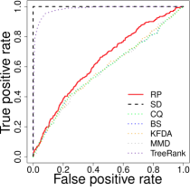
(a) font=Large

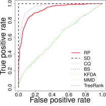
(b) diagonal $\Sigma$, fast decay

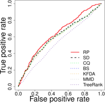
(c) random $\Sigma$, slow decay

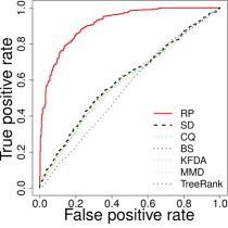
(d) random $\Sigma$, fast decay

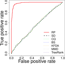
(e) block-diagonal correlation

Figure 3: ROC curves of several test statistics for five different settings of correlation structure and spectral decay of $\Sigma$: (a) Diagonal covariance / slow decay, (b) Diagonal covariance / fast decay, (c) Random covariance / slow decay, and (d) Random covariance / fast decay. (e) Block-diagonal correlation.

On a qualitative level, Figure 3 reveals some striking differences between our procedure and the competing tests. Comparing independent variables versus correlated variables, i.e. panels (a) and (b), with panels (c) and (d), we see that the tests of SD and TreeRank lose power in the presence of correlated data. Meanwhile, the ROC curve of our test is essentially unchanged when passing from independent variables to correlated variables. Similarly, our test also exhibits a large advantage when the correlation structure is prescribed in a block-diagonal manner in panel (e). The agreement of this effect with Theorem 3 is explained in the remarks and examples after that theorem. Comparing slow spectral decay versus fast spectral decay, i.e. panels (a) and (c), with panels (b) and (d), we see that the competing tests are essentially insensitive to the change in spectrum, whereas our test is able to take advantage of low-dimensional covariance structure. The remarks and examples of Theorem 2 give a theoretical justification for this observation.

It is also possible to offer a more quantitative assessment of the ROC curves in light of Theorems  2 and 3. Table 1 summarizes approximate values of $\operatorname{tr}(\Sigma)^{2}/\left|\kern-1.5pt\left|\kern-1.5pt\left|\Sigma\right|\kern-1.5pt\right|\kern-1.5pt\right|_{F}^{2}$ and $\left(\frac{\operatorname{tr}(\Sigma)}{p}\right)^{2}\left(\frac{\operatorname{tr}(D_{\sigma}^{-1})}{\left|\kern-1.5pt\left|\kern-1.5pt\left|R\right|\kern-1.5pt\right|\kern-1.5pt\right|_{F}}\right)^{2}$ from Theorems 2 and 3 in the five settings described above. The table shows that our theory is consistent with Figure 3  in the sense that the only settings for which our test yields an inferior ROC curve are those for which the quantity $\left(\frac{\operatorname{tr}(\Sigma)}{p}\right)^{2}\left(\frac{\operatorname{tr}(D_{\sigma}^{-1})}{\left|\kern-1.5pt\left|\kern-1.5pt\left|R\right|\kern-1.5pt\right|\kern-1.5pt\right|_{F}}\right)^{2}$ is drastically larger than $n=50+50-2=98$. (In all of the settings where $\operatorname{tr}(\Sigma)^{2}/\left|\kern-1.5pt\left|\kern-1.5pt\left|\Sigma\right|\kern-1.5pt\right|\kern-1.5pt\right|_{F}^{2}$ and $\left(\frac{\operatorname{tr}(\Sigma)}{p}\right)^{2}\left(\frac{\operatorname{tr}(D_{\sigma}^{-1})}{\left|\kern-1.5pt\left|\kern-1.5pt\left|R\right|\kern-1.5pt\right|\kern-1.5pt\right|_{F}}\right)^{2}$ are less than $n$, our test yields the best ROC curve against the competitors.) However, if the entries in the table are multiplied by a choice of the constant $c_{1}(\epsilon_{1})>\frac{4}{\epsilon_{1}(1-\sqrt{a})^{4}}$ from Theorems 2 and 3, we see that our asymptotic conditions (14) and (20) are somewhat conservative at the finite sample level. Considering $n=98$, the table shows that $c_{1}(\epsilon_{1})$ would need to be roughly equal to 1.5 so that the inequalities (14) and (20) hold in all the settings for which our method has a better ROC curve than the relevant competitor. In the basic case that $\epsilon_{1}=1$ and $a=0$, we have $\frac{4}{\epsilon_{1}(1-\sqrt{a})^{4}}=4$, which means that the constant $\frac{4}{\epsilon_{1}(1-\sqrt{a})^{4}}$ needs to be improved by roughly a factor of $4/1.5\simeq 3$ or better. We expect that such improvement is possible with a more refined analysis of the proof of Proposition 1.

Table 1: Approximate values of the quantities $\operatorname{tr}(\Sigma)^{2}/\left|\kern-1.5pt\left|\kern-1.5pt\left|\Sigma\right|\kern-1.5pt\right|\kern-1.5pt\right|_{F}^{2}$ and $\left(\frac{\operatorname{tr}(\Sigma)}{p}\right)^{2}\left(\frac{\operatorname{tr}(D_{\sigma}^{-1})}{\left|\kern-1.5pt\left|\kern-1.5pt\left|R\right|\kern-1.5pt\right|\kern-1.5pt\right|_{F}}\right)^{2}$ in the five parameter settings of the synthetic data experiments. Theorems 2 and 3 assert that these quantities determine the relative performance of our test against CQ and SD respectively.

	diagonal $\Sigma$,	diagonal $\Sigma$,	random $\Sigma$,	random $\Sigma$,	block-diagonal
	slow decay	fast decay	slow decay	fast decay	correlation
(Thm. 2 vs. CQ)   $\operatorname{tr}(\Sigma)^{2}/\left|\kern-1.5pt\left|\kern-1.5pt\left|\Sigma\right|\kern-1.5pt\right|\kern-1.5pt\right|_{F}^{2}$	54	25	54	25	41
(Thm. 3 vs. SD) $\left(\frac{\operatorname{tr}(\Sigma)}{p}\right)^{2}\left(\frac{\operatorname{tr}(D_{\sigma}^{-1})}{\left|\kern-1.5pt\left|\kern-1.5pt\left|R\right|\kern-1.5pt\right|\kern-1.5pt\right|_{F}}\right)^{2}$	$4.6\times 10^{5}$	$3.5\times 10^{5}$	58	30	41

4.2 Calibration curves on synthetic data

Figure 4 contains calibration plots resulting from the simulations described in Section 4.1—showing how well the observed false positive rates (FPR) of the various tests compare against the nominal level $\alpha$. (Note that these plots only reflect simulations under ${\bf{H}}_{0}$.) Ideally, when testing at level $\alpha$, the observed FPR should be as close to $\alpha$ as possible, and a thin diagonal grey line is used here as a reference for perfect calibration. Figures 4 (a) and (b) correspond respectively to the settings from Section 4.1 where $\Sigma$ is diagonal, with a slowly decaying spectrum, and where $\Sigma$ has random eigenvectors and a rapidly decaying spectrum. In these cases the tests of BS, CQ, and SD are reasonably well-calibrated, and our test is nearly on top of the optimal diagonal line. To consider robustness of calibration, we repeated the simulation from panel (a), but replaced the sampling distributions $N(\mu_{i},\Sigma)$, $i=1,2$, with the mixtures $0.2\,N(\mu_{i}+d_{1,i},\Sigma)+0.3\,N(\mu_{i}+d_{2,i},\Sigma)+0.5\,N(\mu_{i}+d_{3,i},\Sigma)$, where $0.2\,d_{1,i}+0.3\,d_{2,i}+0.5\,d_{3,i}=0$, and $d_{1,1},d_{2,1},d_{1,2},d_{2,2}$ were drawn independently and uniformly from a sphere of radius $\left|\kern-1.5pt\left|\kern-1.5pt\left|\Sigma\right|\kern-1.5pt\right|\kern-1.5pt\right|_{F}^{2}$. The resulting calibration plot in Figure 4 (c) shows that our test deviates slightly from the diagonal in this case, but the calibration of the other three tests degrades to a much more noticeable extent. Experiments on other non-Gaussian distributions (e.g. with heavy tails) gave similar results, suggesting that the critical values of our procedure may be generally more robust (see also the discussions of robustness in Sections 2.1 and 4.3).

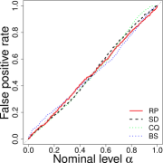
(a) font=Large

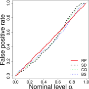
(b) font=Large

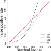
(c) font=Large

Figure 4: Calibration plots on synthetic data under three different data-generating distributions. The grey line is a reference for optimal calibration.

4.3 Comparison on high-dimensional gene expression data.

The ability to detect gene sets having different expression between two types of conditions, e.g., benign and malignant forms of a disease, is of great value in many areas of biomedical research. In this section, we study our testing procedure in the context of determining whether a set of $p$ genes is differentially expressed between two relatively small groups of patients of sizes $n_{1}$ and $n_{2}$. To compare the performance of our $T_{k}^{2}$ statistic against competitors CQ and SD in this type of application, we constructed a collection of 1680 distinct two-sample problems in the following manner, using data from three genomic studies of ovarian (Tothill2008Novel, ), myeloma (Moreaux2011high-risk, ) and colorectal (Jorissen2009Metastasis-Associated, ) cancers. First, we randomly split the 3 datasets respectively into $6$, $4$, and $6$ groups of approximately $50$ patients. Next, we considered all possible pairwise comparisons between all sets of patients on each of 14 biologically meaningful gene sets from the canonical pathways of the database MSigDB (Subramanian2005Gene, ). Each gene set contains between $75$ and $128$ genes (with an average of $98.5$). Since $n_{1}\simeq n_{2}\simeq 50$, our collection of two-sample problems is genuinely high-dimensional. Specifically, we have $14\times(\binom{6}{2}+\binom{4}{2}+\binom{6}{2})=504$ problems under ${\bf{H}}_{0}$, and $14\times(6\times 4+6\times 4+6\times 6)=1176$ problems under ${\bf{H}}_{1}$, where we assume that every gene set is differentially expressed between two sets of patients with two different cancers, and that no gene set is differentially expressed between two sets of patients with the same cancer. Although it is conceivable that this assumption could be violated by the existence of various cancer subtypes, or differences between original tissue samples, our initial step of randomly splitting the three cancer datasets into subsets guards against this possibility.

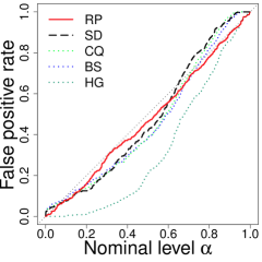
(a) FPR for genomic data

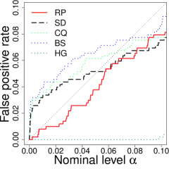
(b) FPR for genomic data (zoom)

Figure 5: (a) False positive rate against p-value threshold on the gene expression experiment of Section 4.3 for RP, BS, CQ, SD and the hypergeometric (HG) enrichment test. (b) Zoom on the $\textrm{p-value}<0.1$ region. The optimal diagonal line is plotted in light grey.

With consideration to ROC curves, the cancer datasets are dissimilar enough that BS, CQ, SD, and our method all produce perfect ROC curves from the collection of two-sample problems (no ${\bf{H}}_{1}$ case has a larger p-value than any ${\bf{H}}_{0}$ case). The hypergeometric test-based (HG) enrichment analysis (Beissbarth2004GOstat, ) often used by experimentalists on this problem gives a suboptimal area-under-curve of $0.989$.

Examining the quality of calibration reveals an important difference between our test and the competitors in this example. It is apparent in Figure 5 (a) that the curve for our procedure is closer to the optimal diagonal line (plotted in light grey) for most values of $\alpha$ than the competing curves. Furthermore, the lower-left corner of Figure  5 (a) is of particular importance, as practitioners are usually only interested in p-values lower than $10^{-1}$. Figure 5 (b) is a zoomed plot of the lower-left corner, which shows that the SD and CQ tests commit too many false positives at low thresholds. Again, in this regime, our procedure is closer to the diagonal and safely commits fewer than the allowed number of false positives. For example, when thresholding p-values at $0.01$, SD has an actual FPR of $0.03$, and an even more excessive FPR of $0.02$ when thresholding at $0.001$. The tests of CQ and BS do even worse. The same thresholds on the p-values of our test lead to false positive rates of $0.008$ and $0$ respectively.

As discussed in Section 2.1, there are two properties of our testing procedure that could account for the advantage of our FPR on the both the synthetic and real data. First, our test inherits exact critical values for Gaussian data from the classical Hotelling test, whereas the competing tests of SD, CQ, and BS use thresholds based on asymptotic approximations. Second, even if the $p$-dimensional data is poorly approximated by $N(\mu_{1},\Sigma)$ and $N(\mu_{1},\Sigma)$, it is well known that randomly projected data tends to be nearly Gaussian FreedmanDiaconis . Consequently, the use of a projection that induces Gaussianity, in conjunction with exact critical values for Gaussian data may explain the advantage of our test’s FPR.

5 Conclusion

We have proposed a novel testing procedure for the two-sample test of means in high dimensions. This procedure can be implemented in a simple manner by first projecting a dataset with a single randomly drawn matrix, and then applying the standard Hotelling $T^{2}$ test in the projected space. In addition to deriving an asymptotic power function for this test, we have provided interpretable conditions on the covariance and correlation matrices for achieving greater power than competing tests in the sense of asymptotic relative efficiency. Specifically, our theoretical comparisons show that our test is well-suited to interesting regimes where the data variables are correlated, or where most of the variance can be captured in a small number of variables. Furthermore, in the realistic case of $(n,p)=(100,200)$, these types of conditions were shown to correspond to favorable performance of our test against several competitors in ROC curve comparisons on synthetic data. Finally, we showed on real gene expression data that our procedure was more reliable than competitors in terms of its false positive rate. Extensions of this work may include more refined applications of random projection to other high-dimensional testing problems.

Acknowledgements.

The authors thank Sandrine Dudoit, Anne Biton, and Peter Bickel for helpful discussions. MEL gratefully acknowledges the support of the DOE CSGF Fellowship, under grant number DE-FG02-97ER25308, and LJJ the support of Stand Up to Cancer. MJW was partially supported by NSF grant DMS-0907632.

Appendix A Matrix and Concentration Inequalities

This appendix is devoted to a number of matrix and concentration inequalities used at various points in our analysis. We also prove Lemma 1, which is stated in the main text in Section 3.5.

Lemma 2.

If $A$ and $B$ are square real matrices of the same size with $A\succeq 0$ and $B=B^{\top}$, then

$$\lambda_{\min}(B)\operatorname{tr}(A)\leq\operatorname{tr}(AB)\leq\lambda_{\max}(B)\operatorname{tr}(A).$$ (30)

Proof. The upper bound is an immediate consequence of Fan’s inequality (BorweinLewis, , p.10), which states that any two symmetric matrices $A,B\in\mathbb{R}^{p\times p}$ satisfy $\operatorname{tr}(AB)\leq\sum_{i=1}^{p}\lambda_{i}(A)\lambda_{i}(B),$ where $\lambda_{i+1}(\cdot)\leq\lambda_{i}(\cdot)$. Replacing $A$ with $-A$ yields the lower bound. ∎

See the papers of Bechar Bechar , or Laurent and Massart LaurentMassart for proofs of the following concentration bounds for Gaussian quadratic forms.

Lemma 3.

Let $A\in\mathbb{R}^{p\times p}$ with $A\succeq 0$, and $Z\sim N(0,I_{p\times p})$. Then for any $t>0$, we have

$$\mathbb{P}\left[Z^{\top}AZ\geq\operatorname{tr}(A)+2\left|\kern-1.5pt\left|\kern-1.5pt\left|A\right|\kern-1.5pt\right|\kern-1.5pt\right|_{F}\sqrt{t}+2\left|\kern-1.5pt\left|\kern-1.5pt\left|A\right|\kern-1.5pt\right|\kern-1.5pt\right|_{2}t\right] \;\leq\;\exp(-t),\quad\mbox{and}$$ (31a)

$$\mathbb{P}\left[Z^{\top}AZ\leq\operatorname{tr}(A)-2\left|\kern-1.5pt\left|\kern-1.5pt\left|A\right|\kern-1.5pt\right|\kern-1.5pt\right|_{F}\sqrt{t}\right] \;\leq\;\exp(-t).$$ (31b)

The following result on the extreme eigenvalues of Wishart matrices is given in Davidson and Szarek (DavidsonSzarek, , Theorem II.13).

Lemma 4.

For $k\leq p$, let $P_{k}^{\top}\in\mathbb{R}^{k\times p}$ be a random matrix with i.i.d. $N(0,1)$ entries. Then, for all $t>0$, we have

$$\textstyle\mathbb{P}\left[\lambda_{\max}\big{(}\frac{1}{p}P_{k}^{\top}P_{k}\right)\geq\left(1+\sqrt{k/p}+t\big{)}^{2}\right] \leq\exp(-pt^{2}/2),\quad\mbox{and}$$ (32a)

$$\textstyle\mathbb{P}\left[\lambda_{\min}\big{(}\frac{1}{p}P_{k}^{\top}P_{k}\big{)}\leq\big{(}1-\sqrt{k/p}-t\big{)}^{2}\right] \leq\exp(-pt^{2}/2).$$ (32b)

Proof of Lemma 1. Note that the function $f(Z):=\sqrt{Z^{\top}AZ}=\|A^{1/2}Z\|_{2}$ has Lipschitz constant $\left|\kern-1.5pt\left|\kern-1.5pt\left|A^{1/2}\right|\kern-1.5pt\right|\kern-1.5pt\right|_{2}=\sqrt{\left|\kern-1.5pt\left|\kern-1.5pt\left|A\right|\kern-1.5pt\right|\kern-1.5pt\right|_{2}}$ with respect to the Euclidean norm on $\mathbb{R}^{p}$. By the Gaussian isoperimetric inequality Massart , we have for any $s>0$,

$$\mathbb{P}\left[f(Z)\leq\mathbb{E}[f(Z)]-s\right]\leq\exp\left(\textstyle{\frac{-s^{2}}{2\left|\kern-1.5pt\left|\kern-1.5pt\left|A\right|\kern-1.5pt\right|\kern-1.5pt\right|_{2}}}\right).$$ (33)

From the Poincaré inequality for Gaussian measures Beckner , the variance of $f(Z)$ is bounded above as $\operatorname{Var}[f(Z)]\leq\left|\kern-1.5pt\left|\kern-1.5pt\left|A\right|\kern-1.5pt\right|\kern-1.5pt\right|_{2}$. Noting that $\mathbb{E}[f(Z)^{2}]=\operatorname{tr}(A)$, we see that the expectation of $f(Z)$ is lower bounded as

$$\mathbb{E}[f(Z)]\geq\sqrt{\operatorname{tr}(A)-\left|\kern-1.5pt\left|\kern-1.5pt\left|A\right|\kern-1.5pt\right|\kern-1.5pt\right|_{2}}.$$

Substituting this lower bound into the concentration inequality (33) yields

$$\mathbb{P}\left[f(Z)\leq\sqrt{\operatorname{tr}(A)-\left|\kern-1.5pt\left|\kern-1.5pt\left|A\right|\kern-1.5pt\right|\kern-1.5pt\right|_{2}}-s\right]\leq\exp\left(\textstyle{\frac{-s^{2}}{2\left|\kern-1.5pt\left|\kern-1.5pt\left|A\right|\kern-1.5pt\right|\kern-1.5pt\right|_{2}}}\right).$$

Finally, letting $t\in\left(0,\sqrt{\frac{\operatorname{tr}(A)}{\left|\kern-1.5pt\left|\kern-1.5pt\left|A\right|\kern-1.5pt\right|\kern-1.5pt\right|_{2}}-1}\right)$, and choosing $s^{2}=t^{2}\left|\kern-1.5pt\left|\kern-1.5pt\left|A\right|\kern-1.5pt\right|\kern-1.5pt\right|_{2}$ yields the claim (24).

The Gaussian isoperimetric inequality also implies $\mathbb{P}\left[f(Z)\geq\mathbb{E}f(Z)+s\right]\leq\exp\left(\textstyle{\frac{-s^{2}}{2\left|\kern-1.5pt\left|\kern-1.5pt\left|A\right|\kern-1.5pt\right|\kern-1.5pt\right|_{2}}}\right)$. By Jensen’s inequality, we have

$$\mathbb{E}[f(Z)]=\mathbb{E}\sqrt{Z^{\top}AZ}\leq\sqrt{\mathbb{E}[Z^{\top}AZ]}=\sqrt{\operatorname{tr}(A)},$$

from which we obtain $\mathbb{P}\left[f(Z)\geq\sqrt{\operatorname{tr}(A)}+s\right]\leq\exp\left(\textstyle{\frac{-s^{2}}{2\left|\kern-1.5pt\left|\kern-1.5pt\left|A\right|\kern-1.5pt\right|\kern-1.5pt\right|_{2}}}\right)$, and setting $s^{2}=t^{2}\left|\kern-1.5pt\left|\kern-1.5pt\left|A\right|\kern-1.5pt\right|\kern-1.5pt\right|_{2}$ for $t>0$ yields the claim (23).

Appendix B Proof of Proposition 1

The proof of Proposition 1 is based on Lemmas 5 and 6, which we state and prove below in Section B.1. We then prove Proposition 1 in two parts, by first proving the lower bound (11a), and then the upper bound (11b) in sections B.2 and B.3 respectively.

B.1 Two auxiliary lemmas

Note that the following two lemmas only deal with the randomness in the $k\times p$ matrix $P_{k}^{\top}$, and they can be stated without reference to the sample size $n$.

Lemma 5.

Let $P_{k}^{\top}\in\mathbb{R}^{k\times p}$ have i.i.d. $N(0,1)$ entries, where $k\leq p$. Assume there is a constant $a\in[0,1)$ such that $k/p\to a$ as $(k,p)\to\infty$. Then, there is a sequence of numbers $c_{k}\to(1-\sqrt{a})^{2}$ such that

$$\mathbb{P}\left[\frac{1}{p}\operatorname{tr}(P_{k}(P_{k}^{\top}\Sigma P_{k})^{-1}P_{k}^{\top})\geq\frac{k}{\operatorname{tr}(\Sigma)}c_{k}\right]\to 1\text{ as }(k,p)\to\infty.$$

Proof. By the cyclic property of trace and Lemma 2, we have

$$\frac{1}{p}\operatorname{tr}\left(P_{k}(P_{k}^{\top}\Sigma P_{k})^{-1}P_{k}^{\top}\right) =\frac{1}{p}\operatorname{tr}\left((P_{k}^{\top}\Sigma P_{k})^{-1}P_{k}^{\top}P_{k}\right)$$ (34)

$$\geq\frac{1}{p}\operatorname{tr}\left((P_{k}^{\top}\Sigma P_{k})^{-1}\right)\lambda_{\min}\left(P_{k}^{\top}P_{k}\right).$$ (35)

For a general positive-definite matrix $A\in\mathbb{R}^{k\times k}$, Jensen’s inequality implies $\operatorname{tr}(A^{-1})\geq k^{2}/\operatorname{tr}(A)$. Combining this with the lower-bound on $\lambda_{\min}(P_{k}^{\top}P_{k})$ from Lemma (4) leads to

$$\frac{1}{p}\operatorname{tr}\left(P_{k}(P_{k}^{\top}\Sigma P_{k})^{-1}P_{k}^{\top}\right)\geq\frac{k^{2}}{\operatorname{tr}(P_{k}^{\top}\Sigma P_{k})}\cdot\underbrace{[1-\sqrt{k/p}-t_{2}]^{2}}_{=:1-r_{2}(t_{2})},$$ (36)

with probability at least $1-\exp(-pt_{2}^{2}/2)$.

We now obtain a high-probability upper bound on $\operatorname{tr}(P_{k}^{\top}\Sigma P_{k})$ that is of order $k\,\operatorname{tr}(\Sigma)$. First let $\Sigma=U\Lambda U^{\top}$ be a spectral decomposition of $\Sigma$. Writing $P_{k}^{\top}\Sigma P_{k}$ as $(P_{k}^{\top}U)\Lambda(U^{\top}P_{k})$, and recalling that the columns of $P_{k}$ are distributed as $N(0,I_{p\times p})$, we see that $P_{k}^{\top}\Sigma P_{k}$ is distributed as $P_{k}^{\top}\Lambda P_{k}$. Hence, we may work under the assumption that $\Sigma$ and $\Lambda$ are interchangeable. Let $0<\lambda_{1}\leq\cdots\leq\lambda_{p}$ be the eigenvalues of $\Sigma$, with $\lambda_{i}=\Lambda_{ii}$, and let ${\bf{Z}}\in\mathbb{R}^{(pk)\times 1}$ be a concatenated column vector of $k$ independent and identically distributed $N(0,I_{p\times p})$ vectors. Likewise, let ${\bf{\Lambda}}\in\mathbb{R}^{pk\times pk}$ be a diagonal matrix obtained by arranging $k$ copies of $\Lambda$ along the diagonal, i.e.

$$\bf{\Lambda} :\,=\left(\begin{array}[]{ccc}\Lambda&&\\ &\ddots&\\ &&\Lambda\end{array}\right).$$ (40)

By considering the diagonal entries of $P_{k}^{\top}\Lambda P_{k}$, it is straightforward to verify that $\operatorname{tr}(P_{k}^{\top}\Lambda P_{k})\stackrel{{\scriptstyle d}}{{=}}\bf{Z}^{\top}\bf{\Lambda}\bf{Z}.$ Applying Lemma 3 to the quadratic form $\bf{Z}^{\top}\bf{\Lambda}\bf{Z},$ and noting that $\left|\kern-1.5pt\left|\kern-1.5pt\left|\Lambda\right|\kern-1.5pt\right|\kern-1.5pt\right|_{F}/\operatorname{tr}(\Lambda)$ and $\left|\kern-1.5pt\left|\kern-1.5pt\left|\Lambda\right|\kern-1.5pt\right|\kern-1.5pt\right|_{2}/\operatorname{tr}(\Lambda)$ are at most 1, we have

$$\begin{split}\operatorname{tr}(P_{k}^{\top}\Lambda P_{k})&\leq\operatorname{tr}({\bf{\Lambda}})+2\sqrt{t_{3}}\small{\left|\kern-1.5pt\left|\kern-1.5pt\left|\bf{\Lambda}\right|\kern-1.5pt\right|\kern-1.5pt\right|_{F}}+2t_{3}\left|\kern-1.5pt\left|\kern-1.5pt\left|{\bf{\Lambda}}\right|\kern-1.5pt\right|\kern-1.5pt\right|_{2}\\ &=k\operatorname{tr}(\Lambda)+2\sqrt{t_{3}}\sqrt{k}\left|\kern-1.5pt\left|\kern-1.5pt\left|\Lambda\right|\kern-1.5pt\right|\kern-1.5pt\right|_{F}+2t_{3}\left|\kern-1.5pt\left|\kern-1.5pt\left|\Lambda\right|\kern-1.5pt\right|\kern-1.5pt\right|_{2}\\ &\footnotesize{\leq k\operatorname{tr}(\Lambda)\underbrace{\left(1+\frac{2\sqrt{t_{3}}}{\sqrt{k}}+\frac{2t_{3}}{k}\right)}_{=:1+r_{3}(t_{3})},}\\ \end{split}$$ (41)

with probability at least $1-\exp(-t_{3})$, giving the desired upper bound on $\operatorname{tr}(P_{k}^{\top}\Lambda P_{k})$. In order to combine the last bound with (36), define the event

$$E_{k} :\,=\left\{\frac{1}{p}\operatorname{tr}\left(P_{k}(P_{k}^{\top}\Sigma P_{k})^{-1}P_{k}^{\top}\right)\geq\frac{k}{\operatorname{tr}(\Sigma)}\frac{1-r_{2}(t_{2})}{1+r_{3}(t_{3})}\right\},$$

and then observe that $\mathbb{P}(E_{k})\geq 1-\exp(-pt_{2}^{2}/2)-\exp(-t_{3})$ by the union bound. Choosing $t_{2}=1/p^{1/4}$ and $t_{3}=\sqrt{k}$, we ensure that $\mathbb{P}(E_{k})\to 1$ as $(k,p)\to\infty$, and moreover, that

$$\frac{1-r_{2}(t_{2})}{1+r_{3}(t_{3})}\to(1-\sqrt{a})^{2},\\$$

which completes the proof. ∎

Lemma 6.

Assume the conditions of Lemma 5. Then for any $C>\frac{(1+\sqrt{a})^{2}}{(1-\sqrt{a})^{2}}$, we have

$$\mathbb{P}\left[\left|\kern-1.5pt\left|\kern-1.5pt\left|P_{k}(P_{k}^{\top}\Sigma P_{k})^{-1}P_{k}^{\top}\right|\kern-1.5pt\right|\kern-1.5pt\right|_{F}\leq\frac{C\sqrt{k}}{\lambda_{\min}(\Sigma)}\right] \to 1\quad\mbox{as $(k,p)\to\infty$.}$$ (42)

Proof. By the relation $\left|\kern-1.5pt\left|\kern-1.5pt\left|A\right|\kern-1.5pt\right|\kern-1.5pt\right|_{F}^{2}=\operatorname{tr}(A^{2})$ for symmetric matrices $A$, and the cyclic property of trace,

$$\left|\kern-1.5pt\left|\kern-1.5pt\left|P_{k}(P_{k}^{\top}\Sigma P_{k})^{-1}P_{k}^{\top}\right|\kern-1.5pt\right|\kern-1.5pt\right|_{F}^{2} =\operatorname{tr}\left(\left(P_{k}(P_{k}^{\top}\Sigma P_{k})^{-1}P_{k}^{\top}\right)^{2}\right)\;=\;\operatorname{tr}\left(\left((P_{k}^{\top}\Sigma P_{k})^{-1}P_{k}^{\top}P_{k}\right)^{2}\right).$$

Letting $\rho(\cdot)$ denote the spectral radius of a matrix, we use the fact that $|\operatorname{tr}(A)|\leq k\rho(A)\leq k\left|\kern-1.5pt\left|\kern-1.5pt\left|A\right|\kern-1.5pt\right|\kern-1.5pt\right|_{2}$ for all real $k\times k$ matrices $A$ (see (HornJohnson, , p. 297)) to obtain

$$\left|\kern-1.5pt\left|\kern-1.5pt\left|P_{k}(P_{k}^{\top}\Sigma P_{k})^{-1}P_{k}^{\top}\right|\kern-1.5pt\right|\kern-1.5pt\right|_{F}^{2}\leq k\left|\kern-1.5pt\left|\kern-1.5pt\left|\left((P_{k}^{\top}\Sigma P_{k})^{-1}P_{k}^{\top}P_{k}\right)^{2}\right|\kern-1.5pt\right|\kern-1.5pt\right|_{2}.$$

Using the submultiplicative property of $\left|\kern-1.5pt\left|\kern-1.5pt\left|\cdot\right|\kern-1.5pt\right|\kern-1.5pt\right|_{2}$ twice in succession,

$$\begin{split}\left|\kern-1.5pt\left|\kern-1.5pt\left|P_{k}(P_{k}^{\top}\Sigma P_{k})^{-1}P_{k}^{\top}\right|\kern-1.5pt\right|\kern-1.5pt\right|_{F}^{2}&\leq k\left|\kern-1.5pt\left|\kern-1.5pt\left|(P_{k}^{\top}\Sigma P_{k})^{-1}P_{k}^{\top}P_{k}\right|\kern-1.5pt\right|\kern-1.5pt\right|_{2}^{2}\\ &\leq k\left|\kern-1.5pt\left|\kern-1.5pt\left|(P_{k}^{\top}\Sigma P_{k})^{-1}\right|\kern-1.5pt\right|\kern-1.5pt\right|_{2}^{2}\cdot\left|\kern-1.5pt\left|\kern-1.5pt\left|P_{k}^{\top}P_{k}\right|\kern-1.5pt\right|\kern-1.5pt\right|_{2}^{2}\\ &=k\frac{1}{\lambda^{2}_{\min}(P_{k}^{\top}\Sigma P_{k})}\cdot\lambda_{\max}^{2}(P_{k}^{\top}P_{k}).\end{split}$$ (43)

Next, by Lemma 4, we have the bound

$$\lambda_{\max}(P_{k}^{\top}P_{k})\leq p\cdot\underbrace{[1+\sqrt{k/p}+t_{4}]^{2}}_{=:1+r_{4}(t_{4})},$$ (44)

with probability at least $1-\exp(-pt_{4}^{2}/2)$.

By the variational characterization of eigenvalues, followed by Lemma 4, we have

$$\begin{split}\lambda_{\min}(P_{k}^{\top}\Sigma P_{k})&=\inf_{\|x\|_{2}=1}\left(x^{\top}P_{k}^{\top}\Sigma P_{k}x\right)\\ &\geq\inf_{\|y\|_{2}=1}\left(y^{\top}\Sigma y\right)\inf_{\|x\|_{2}=1}\|P_{k}x\|_{2}^{2}\\ &=\lambda_{\min}(\Sigma)\cdot\lambda_{\min}(P_{k}^{\top}P_{k})\\ &\geq\lambda_{\min}(\Sigma)\cdot p\cdot(1-r_{2}(t_{2})),\\ \end{split}$$ (45)

with probability at least $1-\exp(-pt_{2}^{2}/2),$ and $r_{2}(t_{2})$ defined as in line (36).

Substituting the bounds (44) and (45) into line (43), we obtain

$$\begin{split}\left|\kern-1.5pt\left|\kern-1.5pt\left|P_{k}(P_{k}^{\top}\Sigma P_{k})^{-1}P_{k}^{\top}\right|\kern-1.5pt\right|\kern-1.5pt\right|_{F}^{2}\leq\frac{k}{\lambda^{2}_{\min}(\Sigma)}\frac{(1+r_{4}(t_{4}))^{2}}{(1-r_{2}(t_{2}))^{2}}.\\ \end{split}$$ (46)

with probability at least $1-\exp(-pt_{2}^{2}/2)-\exp(-pt_{4}^{2}/2)$, where we have used the union bound.

Setting $t_{2}=t_{4}=1/p^{1/4}$, the probability of the event (46) tends to 1 as $(k,p)\to\infty$. Furthermore,

$$\frac{(1+r_{4}(t_{4}))^{2}}{(1-r_{2}(t_{2}))^{2}}\to\frac{(1+\sqrt{a})^{4}}{(1-\sqrt{a})^{4}},$$

and so we may take $C$ in the statement of the lemma to be any constant strictly greater than $\frac{(1+\sqrt{a})^{2}}{(1-\sqrt{a})^{2}}$. ∎

B.2 Proof of lower bound (11a) in Proposition 1

By the assumption on the distribution of $\delta$, we may write $\delta/\|\delta\|_{2}$ as $Z/\|Z\|_{2}$ where $Z\sim N(0,I_{p\times p})$. Furthermore, because $\|Z\|_{2}/\sqrt{p}\to 1$ almost surely as $n\to\infty$, it is possible to replace $\delta/\|\delta\|_{2}$ with $Z/\sqrt{p}$, and work under the assumption that $\frac{\Delta_{k}^{2}}{\|\delta\|_{2}^{2}}=\frac{1}{p}Z^{\top}P_{k}(P_{k}^{\top}\Sigma P_{k})^{-1}P_{k}^{\top}Z$. Noting that we may take $Z$ to be independent of $P_{k}^{\top}$, the concentration inequality for Gaussian quadratic forms in Lemma 2 gives a lower bound on the conditional probability

$$\mathbb{P}\left[\textstyle\frac{\Delta_{k}^{2}}{\|\delta\|_{2}^{2}}\geq\frac{1}{p}\operatorname{tr}\left(P_{k}(P_{k}^{\top}\Sigma P_{k})^{-1}P_{k}^{\top}\right)-\psi(t_{1})\Big{\bracevert}P_{k}^{\top}\right]\geq 1-\exp(-t_{1}),$$ (47)

where $\psi(t_{1}):=\frac{2\sqrt{t_{1}}}{p}\left|\kern-1.5pt\left|\kern-1.5pt\left|P_{k}(P_{k}^{\top}\Sigma P_{k})^{-1}P_{k}^{\top}\right|\kern-1.5pt\right|\kern-1.5pt\right|_{F}$ is a random error term, and $t_{1}$ is a positive real number that may vary with $n$. Now that the randomness from $\delta$ has been separated out in (47), we study the randomness from $P_{k}^{\top}$ by defining the event

$$\textstyle\mathcal{E}_{n}:=\left\{\frac{1}{p}\operatorname{tr}\left(P_{k}(P_{k}^{\top}\Sigma P_{k})^{-1}P_{k}^{\top}\right)-\psi(t_{1})\geq L_{n}\right\},$$ (48)

where $L_{n}$ is a real number whose dependence on $n$ will be specified below. To see the main line of argument toward the statement of the proposition, we integrate the conditional probability in line (47) with respect to $P_{k}^{\top}$, and obtain

$$\mathbb{P}\left(\textstyle{\frac{\Delta_{k}^{2}}{\|\delta\|_{2}^{2}}\geq L_{n}}\right)\geq[1-\exp(-t_{1})]\,\mathbb{P}(\mathcal{E}_{n}).$$ (49)

The rest of the proof proceeds in two parts. First, we lower-bound $\operatorname{tr}\left(P_{k}(P_{k}^{\top}\Sigma P_{k})^{-1}P_{k}^{\top}\right)\big{/}p$ on an event $\mathcal{E}_{n}^{\prime}$ with $\mathbb{P}(\mathcal{E}_{n}^{\prime})\to 1$ as $n\to\infty$. Second, we upper-bound $\psi(t_{1})$ on an event $\mathcal{E}_{n}^{\prime\prime}$ with $\mathbb{P}(\mathcal{E}_{n}^{\prime\prime})\to 1$. Then we choose $L_{n}$ so that $\mathcal{E}_{n}\supset\mathcal{E}_{n}^{\prime}\cap\mathcal{E}_{n}^{\prime\prime}$, and take $t_{1}\to\infty$ so that (49) implies $\mathbb{P}(\Delta_{k}^{2}\big{/}\|\delta\|_{2}^{2}\geq L_{n})\to 1$ as $n\to\infty$.

For the first step of lower-bounding $\operatorname{tr}\left(P_{k}(P_{k}^{\top}\Sigma P_{k})^{-1}P_{k}^{\top}\right)\big{/}p$, Lemma 5 asserts that there is a sequence of numbers $c_{n}\to(1-\sqrt{a})^{2}$ such that the event

$$\textstyle\mathcal{E}_{n}^{\prime}:=\left\{\frac{1}{p}\operatorname{tr}\left(P_{k}(P_{k}^{\top}\Sigma P_{k})^{-1}P_{k}^{\top}\right)\geq\frac{k}{\operatorname{tr}(\Sigma)}c_{n}\right\}$$ (50)

satisfies $\mathbb{P}(\mathcal{E}_{n}^{\prime})\to 1$ as $n\to\infty$.

Next, for the second step of upper-bounding the error $\psi(t_{1})$, Lemma 6 guarantees that for any constant $C$ strictly greater than $\frac{(1+\sqrt{a})^{2}}{(1-\sqrt{a})^{2}}$, the event

$$\textstyle\mathcal{E}_{n}^{\prime\prime}:=\left\{\frac{2}{p}\left|\kern-1.5pt\left|\kern-1.5pt\left|P_{k}(P_{k}^{\top}\Sigma P_{k})^{-1}P_{k}^{\top}\right|\kern-1.5pt\right|\kern-1.5pt\right|_{F}\leq\frac{2\,C\sqrt{k}}{p\lambda_{\min}(\Sigma)}\right\}$$ (51)

satisfies $\mathbb{P}(\mathcal{E}_{n}^{\prime\prime})\to 1$ as $n\to\infty$.

Now, with consideration to $\mathcal{E}_{n}^{\prime}$ and $\mathcal{E}_{n}^{\prime\prime}$, define the deterministic quantity

$$\textstyle L_{n}:=\frac{k}{\operatorname{tr}(\Sigma)}\left[c_{n}-\sqrt{t_{1}}\frac{2\,C}{\sqrt{k}}\frac{\operatorname{tr}(\Sigma)}{p\lambda_{\min}(\Sigma)}\right],$$ (52)

which ensures $\mathcal{E}_{n}\supset\mathcal{E}_{n}^{\prime}\cap\mathcal{E}_{n}^{\prime\prime}$ for all choices of $t_{1}$. Consequently, $\mathbb{P}(\mathcal{E}_{n})\to 1$, and it remains to choose $t_{1}$ appropriately so that the probability in line (49) tends to 1. If we let $t_{1}=\sqrt{k}\,\frac{p\,\lambda_{\min}}{\operatorname{tr}(\Sigma)}$, then $t_{1}\to\infty$ by assumption (A5), and the second term inside the brackets in line (52) vanishes as $n\to\infty$. Altogether, we have shown that

$$L_{n}\frac{\operatorname{tr}(\Sigma)}{k}\to(1-\sqrt{a})^{2},\quad\mbox{ and }\quad\mathbb{P}\left(\textstyle{\frac{\Delta_{k}^{2}}{\|\delta\|_{2}^{2}}\geq L_{n}}\right)\to 1.$$

It follows that $\mathbb{P}\left(\frac{\Delta_{k}^{2}}{\|\delta\|_{2}^{2}}\geq\frac{c\,k}{\operatorname{tr}(\Sigma)}\right)\to 1$ for any positive constant $c<(1-\sqrt{a})^{2}$, which completes the proof of the lower bound (11a).∎

B.3 Proof of upper bound (11b) in Proposition 1

As in the proof of the lower bound 11a in Appendix B.2, we may reduce to the case that $\frac{\Delta_{k}^{2}}{\|\delta\|_{2}^{2}}=\frac{1}{p}Z^{\top}P_{k}(P_{k}^{\top}\Sigma P_{k})^{-1}P_{k}^{\top}Z$. Conditioning on $P_{k}^{\top}$, Lemma 3 gives a lower bound on the conditional probability

$$\mathbb{P}\left[\textstyle\frac{\Delta_{k}^{2}}{\|\delta\|_{2}^{2}}\leq\frac{1}{p}\operatorname{tr}\left(P_{k}(P_{k}^{\top}\Sigma P_{k})^{-1}P_{k}^{\top}\right)+\psi(s_{1})+\phi(s_{1})\Big{\bracevert}P_{k}^{\top}\right]\geq 1-\exp(-s_{1}),$$ (53)

where $s_{1}$ is a positive real number that may vary with $n$, and we define

$$\psi(s_{1}):=\frac{2\sqrt{s_{1}}}{p}\left|\kern-1.5pt\left|\kern-1.5pt\left|P_{k}(P_{k}^{\top}\Sigma P_{k})^{-1}P_{k}^{\top}\right|\kern-1.5pt\right|\kern-1.5pt\right|_{F},\quad\text{ }\quad\phi(s_{1}):=\frac{2s_{1}}{p}\left|\kern-1.5pt\left|\kern-1.5pt\left|P_{k}(P_{k}^{\top}\Sigma P_{k})^{-1}P_{k}^{\top}\right|\kern-1.5pt\right|\kern-1.5pt\right|_{2}.$$ (54)

Clearly, $\phi(s_{1})\leq\sqrt{s_{1}}\psi(s_{1})$. Again, as in the proof of the lower bound (11a), we let $U_{n}$ denote an upper bound whose dependence on $n$ will be specified below, and we define an event

$$\mathcal{D}_{n}:=\left\{\frac{1}{p}\operatorname{tr}\left(P_{k}(P_{k}^{\top}\Sigma P_{k})^{-1}P_{k}^{\top}\right)+(1+\sqrt{s_{1}})\,\psi(s_{1})\leq U_{n}\right\},$$ (55)

and integrate with respect to $P_{k}^{\top}$ to obtain

$$\mathbb{P}\left(\frac{\Delta_{k}^{2}}{\|\delta\|_{2}^{2}}\leq U_{n}\right)\geq[1-\exp(-s_{1})]\,\mathbb{P}(\mathcal{D}_{n}).$$ (56)

Continuing along the parallel line of reasoning, we upper-bound $\frac{1}{p}\operatorname{tr}\left(P_{k}(P_{k}^{\top}\Sigma P_{k})^{-1}P_{k}^{\top}\right)$ on an event $\mathcal{D}_{n}^{\prime}$ (defined below) with $\mathbb{P}(\mathcal{D}_{n}^{\prime})\to 1$, and re-use the upper bound of $\psi(s_{1})$ on the event $\mathcal{E}_{n}^{\prime\prime}$ (see line (51)), which was shown to satisfy $\mathbb{P}(\mathcal{E}_{n}^{\prime\prime})\to 1$. Then, we choose $U_{n}$ so that $\mathcal{D}_{n}\supset\mathcal{D}_{n}^{\prime}\cap\mathcal{E}_{n}^{\prime\prime}$, yielding $\mathbb{P}(\mathcal{D}_{n})\to 1$. Lastly, we take $s_{1}\to\infty$ at an appropriate rate so that the probability in line (56) tends to 1.

To define the event $\mathcal{D}_{n}^{\prime}$ for upper-bounding $\frac{1}{p}\operatorname{tr}\left(P_{k}(P_{k}^{\top}\Sigma P_{k})^{-1}P_{k}^{\top}\right)$, note that for a symmetric matrix $A$ with rank $k$, Jensen’s inequality implies $\operatorname{tr}(A)\leq\sqrt{k\operatorname{tr}(A^{2})}$, regardless of the size of $A$. Considering $A=P_{k}(P_{k}^{\top}\Sigma P_{k})^{-1}P_{k}^{\top}$, and $\sqrt{\operatorname{tr}(A^{2})}=\left|\kern-1.5pt\left|\kern-1.5pt\left|A\right|\kern-1.5pt\right|\kern-1.5pt\right|_{F}$, we see that we may choose $\mathcal{D}_{n}^{\prime}=\mathcal{E}_{n}^{\prime\prime}$ from line (51), and on this set we have the inequality,

$$\frac{1}{p}\operatorname{tr}(P_{k}(P_{k}^{\top}\Sigma P_{k})^{-1}P_{k}^{\top})\leq\sqrt{k}\,\frac{C\sqrt{k}}{p\,\lambda_{\min}(\Sigma)},$$ (57)

with probability tending to 1 as $n\to\infty$, as long as $C$ is strictly greater than $\frac{(1+\sqrt{a})^{2}}{(1-\sqrt{a})^{2}}$. In order to guarantee the inclusion $\mathcal{D}_{n}\supset\mathcal{D}_{n}^{\prime}\cap\mathcal{E}_{n}^{\prime\prime}$, we define

$$U_{n}:=\frac{C\,k}{p\,\lambda_{\min}(\Sigma)}\left[1+(s_{1}+\sqrt{s_{1}})\,\frac{2}{\sqrt{k}}\right].$$ (58)

Note that $k=\lfloor n/2\rfloor$ implies $k\to\infty$ as $n\to\infty$, so choosing $s_{1}=k^{1/4}$ ensures that $s_{1}\to\infty$ and the second term inside the brackets in line (58) vanishes. Combining lines (56) and (58), we have

$$\mathbb{P}\left(\frac{\Delta_{k}^{2}}{\|\delta\|_{2}^{2}}\leq U_{n}\right)\to 1,\quad\mbox{ and }\quad U_{n}\,\frac{p\,\lambda_{\min}(\Sigma)}{C\,k}\to 1.$$

It follows that $\mathbb{P}\left(\frac{\Delta_{k}^{2}}{\|\delta\|_{2}^{2}}\leq\frac{C\,k}{p\,\lambda_{\min}(\Sigma)}\right)\to 1$ for any constant $C$ strictly greater than $\frac{(1+\sqrt{a})^{2}}{(1-\sqrt{a})^{2}}$, which completes the proof of the upper bound (11b).∎

References

• [1] Y. Lu, P. Liu, P. Xiao, and H. Deng. Hotelling’s T2 multivariate profiling for detecting differential expression in microarrays. Bioinformatics, 21(14):3105–3113, Jul 2005.
• [2] J. J. Goeman and P. Bühlmann. Analyzing gene expression data in terms of gene sets: methodological issues. Bioinformatics, 23(8):980–987, Apr 2007.
• [3] D. V. D. Ville, T. Blue, and M. Unser. Integrated wavelet processing and spatial statistical testing of fmri data. Neuroimage, 23(4):1472–1485, 2004.
• [4] U. Ruttimann et al. Statistical analysis of functional mri data in the wavelet domain. IEEE Transactions on Medical Imaging, 17(2):142–154, 1998.
• [5] Z. Bai and H. Saranadasa. Effect of high dimension: by an example of a two sample problem. Statistica Sinica, 6:311,329, 1996.
• [6] M. S. Srivastava and M. Du. A test for the mean vector with fewer observations than the dimension. Journal of Multivariate Analysis, 99:386–402, 2008.
• [7] M. S. Srivastava. A test for the mean with fewer observations than the dimension under non-normality. Journal of Multivariate Analysis, 100:518–532, 2009.
• [8] S. X. Chen and Y. L. Qin. A two-sample test for high-dimensional data with applications to gene-set testing. Annals of Statistics, 38(2):808–835, Feb 2010.
• [9] S. Clémençon, M. Depecker, and Vayatis N. AUC optimization and the two-sample problem. In Advances in Neural Information Processing Systems (NIPS 2009), 2009.
• [10] L. Jacob, P. Neuvial, and S. Dudoit. Gains in power from structured two-sample tests of means on graphs. Technical Report arXiv:q-bio/1009.5173v1, arXiv, 2010.
• [11] A. Gretton, K. M. Borgwardt, M. Rasch, B. Schölkop, and A.J. Smola. A kernel method for the two-sample-problem. In B. Schölkopf, J. Platt, and T. Hoffman, editors, Advances in Neural Information Processing Systems 19, pages 513–520. MIT Press, Cambridge, MA, 2007.
• [12] Z. Harchaoui, F. Bach, and E. Moulines. Testing for homogeneity with kernel Fisher discriminant analysis. In John C. Platt, Daphne Koller, Yoram Singer, and Sam T. Roweis, editors, NIPS. MIT Press, 2007.
• [13] R. J. Muirhead. Aspects of Multivariate Statistical Theory. John Wiley & Sons, inc., 1982.
• [14] S. S. Vempala. The Random Projection Method. DIMACS Series in Discrete Mathematics and Theoretical Computer Science. American Mathematical Society, 2004.
• [15] P. Diaconis and D. Freedman. Asymptotics of graphical projection pursuit. Annals of Statistics, 12(3):793–815, 1984.
• [16] A. W. van der Vaart. Asymptotic Statistics. Cambridge, 2007.
• [17] G. Tang and A. Nehorai. The stability of low-rank matrix reconstruction: a constrained singular value view. arXiv:1006.4088, submitted to IEEE Trans. Information Theory, 2010.
• [18] I. Johnstone. On the distribution of the largest eigenvalue in principal components analysis. Annals of Statistics, 29(2):295–327, 2001.
• [19] L. Wasserman. All of Non-Parametric Statistics. Springer Series in Statistics. Springer-Verlag, New York, NY, 2006.
• [20] I. Bechar. A Bernstein-type inequality for stochastic processes of quadratic forms of Gaussian variables. Technical Report arXiv:0909.3595v1, arXiv, 2009.
• [21] B. Laurent and P. Massart. Adaptive estimation of a quadratic functional by model selection. Annals of Statistics, 28(5):1302–1338, 2000.
• [22] G. W. Stewart. The Efficient Generation of Random Orthogonal Matrices with an Application to Condition Estimators. SIAM Journal on Numerical Analysis, 17(3):403–409, 1980.
• [23] R. W. Tothill et al. Novel molecular subtypes of serous and endometrioid ovarian cancer linked to clinical outcome. Clin Cancer Res, 14(16):5198–5208, Aug 2008.
• [24] J. Moreaux et al. A high-risk signature for patients with multiple myeloma established from the molecular classification of human myeloma cell lines. Haematologica, 96(4):574–582, Apr 2011.
• [25] R. N. Jorissen et al. Metastasis-associated gene expression changes predict poor outcomes in patients with dukes stage b and c colorectal cancer. Clin Cancer Res, 15(24):7642–7651, Dec 2009.
• [26] A. Subramanian et al. Gene set enrichment analysis: a knowledge-based approach for interpreting genome-wide expression profiles. Proc. Natl. Acad. Sci. USA, 102(43):15545–15550, Oct 2005.
• [27] T. Beissbarth and T. P. Speed. Gostat: find statistically overrepresented gene ontologies within a group of genes. Bioinformatics, 20(9):1464–1465, Jun 2004.
• [28] A. S. Lewis J. M. Borwein. Convex Analysis and Nonlinear Optimization Theory and Examples. CMS Bookks in Mathematics. Canadian Mathematical Society, 2000.
• [29] K. R. Davidson and S. J. Szarek. Local operator theory, random matrices, and Banach spaces. in Handbook of Banach Spaces, 1, 2001.
• [30] P. Massart. Concentration Inequalities and Model Selection. Lecture Notes in Mathematics: Ecole d’Eté de Probabilités de Saint-Flour XXXIII-2003. Springer, Berlin, Heidelberg, 2007.
• [31] W. Beckner. A generalized Poincaré inequality for Gaussian measures. Proceedings of the American Mathematical Society, 105(2):397–400, 1989.
• [32] R. Horn and C. Johnson. Matrix Analysis. Cambridge University Press, 22nd printing edition, 2009.