A Monte Carlo study of surface critical phenomena: The special point

Abstract

We study the special point in the phase diagram of a semi-infinite system, where the bulk transition is in the three-dimensional Ising universality class. To this end we perform a finite size scaling study of the improved Blume-Capel model on the simple cubic lattice with two different types of surface interactions. In order to check for the effect of leading bulk corrections we have also simulated the spin-1/2 Ising model on the simple cubic lattice. We have accurately estimated the surface enhancement coupling at the special point of these models. We find $y_{t_{1}}=0.718(2)$ and $y_{h_{1}}=1.6465(6)$ for the surface renormalization group exponents of the special transition. These results are compared with previous ones obtained by using field theoretic methods and Monte Carlo simulations of the spin-1/2 Ising model. Furthermore we study the behavior of the surface transition near the special point and finally we discuss films with special boundary conditions at one surface and fixed ones at the other.

I Introduction

In this paper we shall study the special point in the phase diagram of a semi-infinite system. For reviews on surface critical phenomena see refs. BinderS ; Diehl86 ; Diehl97 . Let us briefly recall the basic features of this phase diagram at the example of the spin-1/2 Ising model on the simple cubic lattice and a semi-infinite geometry. It’s reduced Hamiltonian is given by

$$H=-\beta\sum_{<xy>}s_{x}s_{y}-h\sum_{x}s_{x}-\beta_{1}\sum_{<xy>\in S}s_{x}s_{y}-h_{1}\sum_{x\in S}s_{x}\;\;,$$ (1)

where $x$ and $y$ denote sites of the lattice, $<xy>$ is a pair of nearest neighbors and $S$ is the surface of the system. The spin $s_{x}$ at the site $x$ can take either the value $-1$ or $1$. The Boltzmann factor is given by $\exp(-H)$, since the reduced Hamiltonian incorporates the temperature. We define $\beta=J/k_{B}T$, $\beta_{1}=J_{1}/k_{B}T$, where $J$ is the coupling constant in the bulk, $J_{1}$ the excess coupling constant at the surface and $T$ is the temperature. Below we shall refer to $\beta$ and $\beta_{1}$ as the coupling in the bulk and the excess coupling at the surface, respectively. Below we shall consider vanishing external fields $h=h_{1}=0$ in the bulk as well as at the surface.

In figure 1 we have sketched the phase diagram of this system.

Figure 1: Sketch of the phase diagram of the semi-infinite system. On the $x$-axis we plot the coupling $\beta$ of the bulk and on the $y$-axis the excess coupling $\beta_{1}$ of the surface. The phase, where both the boundary spins and those of the bulk are disordered is labelled by A, while the one with disordered bulk and and ordered surface is labelled by B. The phase, where the bulk and the surface are ordered is labelled by C. The line of surface transitions is labelled by S, the line of ordinary transitions by O and the line of extraordinary transitions by E. These three lines meet in the so called special or surface-bulk point that we have labelled by SP. A discussion is given in the text.

For $\beta>\beta_{c}$, where $\beta_{c}$ is the critical coupling of the bulk system, the spins in the bulk are ordered. As a consequence, also the spins at the surface are ordered. At $\beta=0$ the spins at the surface decouple completely from those of the bulk. Hence a two dimensional Ising model remains that undergoes a phase transition at $\beta_{1}=\beta_{c,2D}$. Starting from the point $(0,\beta_{c,2D})$ there is the line of surface transitions, where the spins at the surface order, while those of the bulk remain disordered. This line hits the line $(\beta_{c},\beta_{1})$ in the so called special or surface-bulk point, which is a tri-critical point. The transitions from disordered surface and disordered bulk to ordered bulk and ordered surface are called ordinary transitions, while those from disordered bulk and ordered surface to ordered bulk and ordered surface are called extraordinary transitions.

Surface critical phenomena had been studied first by using the mean-field approximation BinderS . The application of field theoretic methods to surface critical phenomena is complicated by the fact that translational invariance is broken by the surface. As a consequence, surface critical exponents are only computed up to $O(\epsilon^{2})$ in the $\epsilon$-expansion Diehl86 ; Diehl97 . Furthermore surface critical phenomena have been studied by using high temperature series expansions, real space renormalization group methods and Monte Carlo simulations of lattice models.

The special point is characterized by the two relevant bulk renormalization group (RG)-exponents $y_{t}$ and $y_{h}$ and the two relevant surface RG-exponents $y_{t_{1}}$ and $y_{h_{1}}$. Similar to the pure bulk case, these RG-exponents can be related to a number of surface critical exponents that characterize the behavior of thermodynamic quantities related to the surface in the neighborhood of the special point BinderS ; Diehl86 ; Diehl97 .

In the present work we locate the special point of three different lattice models and determine the RG-exponents $y_{t_{1}}$ and $y_{h_{1}}$ by using finite size scaling (FSS) Barber methods. In the presence of a surface, typically corrections $\propto L^{-1}$ appear BinderS ; Diehl86 ; Diehl97 , where $L$ is the linear extent of the finite system. Analysing numerical data, it is difficult to disentangle these corrections from leading bulk corrections which are $\propto L^{-\omega}$, where $\omega=0.832(6)$ mycritical . Therefore, in addition to the Ising model we simulate the Blume-Capel model that is a generalization of the Ising model. In addition to $-1$ and $1$ the spin can take the value $0$. The parameter $D$ of the Blume-Capel model controls the density of spins with $s_{x}=0$. It has been shown that for a particular value $D^{*}$ of the parameter $D$ the amplitude of leading corrections to scaling vanishes. See mycritical and refs. therein. The precise definition of the model is given below in section II.

The outline of the paper is the following: First we define the models that we simulate. We summarize results for the critical coupling and the critical exponents of the bulk system. We define the quantities that we have measured and discuss their finite size scaling behavior. The scaling behavior is affected by corrections, which have to be taken into account when analysing Monte Carlo data. Then we report our numerical results: First we have simulated three different models on $L^{3}$ lattices, where $L$ is the linear extend of the lattice. Based on these simulations we determine $\beta_{1,sp}$ for these models and obtain estimates of $y_{t_{1}}$ and $y_{h_{1}}$. Next we study the surface transition in the neighborhood of the special point. Then we discuss the magnetisation profile of films with special boundary conditions at one surface and fixed boundary conditions at the other. Finally we summarize and compare our results for the RG-exponents with those obtained by field theoretic methods and previous simulations of the spin-1/2 Ising model.

II Models and observables

The Blume-Capel model on the simple cubic lattice is characterized by the reduced Hamiltonian

$$H=-\beta\sum_{<xy>}s_{x}s_{y}+D\sum_{x}s_{x}^{2}-h\sum_{x}s_{x}\;\;,$$ (2)

where $x=(x_{0},x_{1},x_{2})$ denotes a site of the lattice. The components $x_{0}$, $x_{1}$ and $x_{2}$ take integer values in the range $1\leq x_{i}\leq L_{i}$. The spin $s_{x}$ might take the values $-1$, $0$ or $1$. In the following we shall consider a vanishing external field $h=0$ throughout. The parameter $D$ controls the density of vacancies $s_{x}=0$. In the limit $D\rightarrow-\infty$, these vacancies are completely suppressed, and hence the spin-1/2 Ising model is recovered. For $-\infty\leq D<D_{tri}$ the model undergoes a second order phase transition in the three-dimensional Ising universality class. For $D>D_{tri}$ the transition is of first order. The most recent estimate for the tri-critical point is $D_{tri}=2.0313(4)$ DeBl04 . Numerically, using Monte Carlo simulations it has been shown that there is a point $(D^{*},\beta_{c}(D^{*}))$ on the line of second order phase transitions, where the amplitude of leading corrections to scaling vanishes. Our most recent estimate is $D^{*}=0.656(20)$ mycritical . In mycritical we have simulated the model at $D=0.655$ close to $\beta_{c}$ on lattices of a linear size up to $L=360$. From a standard finite size scaling analysis of renormalization group invariant quantities such as the Binder cumulant we found

$$\beta_{c}(0.655)=0.387721735(25)$$ (3)

for the critical coupling of the bulk at $D=0.655$. Recent estimates for the critical coupling of the bulk of the spin-1/2 Ising model are $\beta_{c}=0.22165455(3)$, table X of DeBl03X and $0.22165463(8)$ mycritical . In the following we assume $\beta_{c}=0.2216546$. The amplitude of leading corrections to scaling at $D=0.655$ is at least by a factor of $30$ smaller than for the spin-1/2 Ising model.

Our recent estimates for bulk critical exponents in the three-dimensional Ising universality class are mycritical

$$\nu = 0.63002(10)\;\;,$$ (4)

$$\eta = 0.03627(10)\;\;,$$ (5)

$$\omega = 0.832(6)\;\;.$$ (6)

II.1 Film geometry and boundary conditions

In Monte Carlo simulations we are restricted to finite lattices. Therefore a surface requires a counterpart. This means that we actually study systems with a film geometry. In the ideal case, film geometry means that the system has a finite thickness $L_{0}$, while in the other two directions the thermodynamic limit $L_{1},L_{2}\rightarrow\infty$ is taken. In order to approximate this limit in Monte Carlo simulations, one usually chooses $L_{0}\ll L_{1},L_{2}$ and applies periodic boundary conditions in the $1$ and $2$ directions. Note that we shall simulate lattices with $L_{1}=L_{2}=L$ throughout. As we shall see below, in order to compute surface critical exponents, the condition $L_{0}\ll L_{1},L_{2}$ is not mandatory. Our estimates for the surface critical exponents are actually obtained from simulations of lattices with $L_{0}=L_{1}=L_{2}=L$.

The reduced Hamiltonian of the Blume-Capel model with film geometry is

$$H = -\beta\sum_{<xy>}s_{x}s_{y}+D\sum_{x}s_{x}^{2}-h\sum_{x}s_{x}-\beta_{1}\sum_{<xy>,x_{0}=y_{0}=1}s_{x}s_{y}-\beta_{2}\sum_{<xy>,x_{0}=y_{0}=L_{0}}s_{x}s_{y}$$ (7)

$$+ D_{1}\sum_{x,x_{0}=1}s_{x}^{2}+D_{2}\sum_{x,x_{0}=L_{0}}s_{x}^{2}\;-\;h_{1}\sum_{x,x_{0}=1}s_{x}\;-\;h_{2}\sum_{x,x_{0}=L_{0}}s_{x}\;\;,$$

where we have put the surfaces at $x_{0}=1$ and $x_{0}=L_{0}$. In our convention $<xy>$ runs over all pairs of nearest neighbor sites with fluctuating spins. Note that here the sites $(1,x_{1},x_{2})$ and $(L_{0},x_{1},x_{2})$ are not nearest neighbors as it would be the case for periodic boundary conditions. For each bulk term there is a corresponding surface enhancement term. In our simulations and the analysis of the data we have used the surface couplings

$$\bar{\beta}_{1}=\beta_{1}+\beta\;\;\mbox{and}\;\;\bar{\beta}_{2}=\beta_{2}+\beta$$ (8)

as parameters instead of the excess surface couplings $\beta_{1}$ and $\beta_{2}$.

Note that as long as the bulk transition and the line of surface transitions remain continuous, the qualitative features of the phase diagram that we have discussed in the introduction should remain unchanged. Since the values of $D$, $D+D_{1}$ and $D+D_{2}$ that we shall consider are much smaller than $D_{tri}=2.0313(4)$ DeBl04 and $D_{tri,2D}=1.966(2)$ SiCaPl06 of the two-dimensional Blume-Capel model on the square lattice, this should be the case in our study.

II.2 Observables

Renormalization group invariant quantities are very useful to locate critical or multicritical points. We study the Binder cumulant

$$U_{4}=\frac{\langle m^{4}\rangle}{\langle m^{2}\rangle^{2}}\;\;,$$ (9)

where $m=\sum_{x}s_{x}$. The second moment correlation length is given by

$$\xi_{2nd}=\sqrt{\frac{\chi/F-1}{4\sin^{2}\pi/L}}\;\;,$$ (10)

where

$$F=\frac{1}{L_{0}L^{2}}\left\langle\Big{|}\sum_{x}\exp\left(i\frac{2\pi x_{1,2}}{L_{1,2}}\right)s_{x}\Big{|}^{2}\right\rangle$$ (11)

is the Fourier transform of the correlation function at the lowest non-zero momentum in 1 or 2 direction and $\chi=\langle m^{2}\rangle/(L_{0}L^{2})$ is the magnetic susceptibility. Since in our simulations $L_{1}=L_{2}$, the expectation value of $F$ is identical for the 1 and the 2 direction. In order to reduce the statistical error, we have measured $F$ for both directions and have averaged the results. The ratio $\xi_{2nd}/L$ is renormalization group invariant. The third renormalization group invariant quantity that we consider is the ratio $Z_{a}/Z_{p}$ of partition functions, where $Z_{a}$ is the partition function of a system with anti-periodic boundary conditions in 1 direction and periodic ones in 2 direction or vice versa, while in the case of $Z_{p}$ periodic boundary conditions are imposed in 1 and 2 direction. Also here, since $L_{1}=L_{2}$ in our simulations, we determine $Z_{a}/Z_{p}$ for both choices and average the results. The ratio $Z_{a}/Z_{p}$ of partition functions can be efficiently evaluated using the boundary flip algorithm BF . Here we use a modified version of the boundary flip algorithm as discussed in appendix A 2 of ref. ourXY . In the following we shall refer to the renormalization group invariant quantities $U_{4}$, $Z_{a}/Z_{p}$ and $\xi_{2nd}/L$ using the symbol $R$. For vanishing symmetry breaking fields $h=h_{1}=h_{2}=0$, $D_{1}=D_{2}$ and $\beta_{1}=\beta_{2}$, a renormalization group invariant quantity behaves as

$$R(L_{0},L,\beta,\beta_{1})=q(L/L_{0},t[L_{0}/\xi_{0}]^{y_{t}},t_{1}[L_{0}/\xi_{1,0}]^{y_{t_{1}}})\;\;,$$ (12)

where $t=\beta_{c}-\beta$, $t_{1}=\beta_{1,sp}-\beta_{1}$, $\xi_{0}$ is the amplitude of the correlation length in the high temperature phase and the normalisation factor $\xi_{1,0}$ is still undetermined. In section (III) we have fixed the ratio $L/L_{0}=1$ and have set the bulk coupling to its critical value: $\beta=\beta_{c}$. This allows us to determine the location of the special point $\beta_{1,sp}$ by using the standard crossing method, where $R$ is considered as function of $\beta_{1}$. The behavior of the slope of the renormalization group invariant quantities allows us to determine the surface RG-exponent $y_{t_{1}}$: Taking the derivative with respect to $\beta_{1}$ we get

$$\frac{\partial R(L_{0},L,\beta,\beta_{1})}{\partial\beta_{1}}=Q(L/L_{0},t[L_{0}/\xi_{0}]^{y_{t}},t_{1}[L_{0}/\xi_{1,0}]^{y_{t_{1}}})\;[L_{0}/\xi_{1,0}]^{y_{t_{1}}}$$ (13)

where $Q$ is minus the partial derivative of $q$ with respect to its third argument.

Finally we define the surface susceptibilities for a vanishing surface magnetisation $\langle m_{1}\rangle$:

$$\chi_{11}=\frac{\partial\langle m_{1}\rangle}{\partial h_{1}}=L^{2}\langle m_{1}^{2}\rangle$$ (14)

where

$$m_{1}=\frac{1}{L^{2}}\sum_{x_{1},x_{2}}s_{(1,x_{1},x_{2})}$$ (15)

and

$$\chi_{12}=\frac{\partial\langle m_{1}\rangle}{\partial h_{2}}=L^{2}\langle m_{1}m_{2}\rangle$$ (16)

where

$$m_{2}=\frac{1}{L^{2}}\sum_{x_{1},x_{2}}s_{(L_{0},x_{1},x_{2})}\;\;.$$ (17)

The finite size scaling behavior of these quantities can be inferred from the singular part of the reduced free energy per area of the film. Its scaling form is

$$f_{s}(...,...,...,h_{1},h_{2})=L_{0}^{-d+1}g(L/L_{0},...,...,h_{1}[L_{0}/l_{h_{1}}]^{y_{h_{1}}},h_{2}[L_{0}/l_{h_{2}}]^{y_{h_{2}}})\;\;,$$ (18)

where the constants $l_{h_{1}}$ and $l_{h_{2}}$ remain undetermined here. $y_{h_{1}}$ and $y_{h_{2}}$ are the RG-exponents related to the surface fields. The susceptibilities defined above can be expressed as second derivatives of $f_{s}$ with respect to the surface fields. Taking these derivatives on the right hand side of eq. (18) we arrive at

$$\chi_{11}=\frac{\partial^{2}f_{s}}{\partial h_{1}^{2}}=cL_{0}^{-d+1}[L_{0}/l_{h_{1}}]^{2y_{h_{1}}}$$ (19)

and

$$\chi_{12}=\frac{\partial^{2}f_{s}}{\partial h_{1}\partial h_{2}}=cL_{0}^{-d+1}[L_{0}/l_{h_{1}}]^{y_{h_{1}}}[L_{0}/l_{h_{2}}]^{y_{h_{2}}}\;\;.$$ (20)

In our study below, section III.2, $y_{h_{1}}=y_{h_{2}}$ and $l_{h_{1}}=l_{h_{2}}$, since we have chosen $\beta_{1}=\beta_{2}$, $D_{1}=D_{2}$ and $h_{1}=h_{2}=0$.

II.3 Corrections to scaling

Finite size scaling laws such as eqs. (12,13,19,20) are affected by corrections. These are caused by irrelevant scaling fields, the analytic background in the reduced free energy per area and the fact that e.g. in eq. (12) the arguments of the scaling function $q$ should be actually analytic functions of $t$ and $t_{1}$ that we have linearized here.

The leading bulk correction is $\propto L_{0}^{-\omega}$, where our most recent estimate $\omega=0.832(6)$ obtained from Monte Carlo simulations of the Blume-Capel and the Ising model mycritical is slightly larger than that obtained from field theoretical methods, e.g. $\omega=0.799(11)$ by using perturbation theory in three dimensions fixed and $\omega=0.814(14)$ by using the $\epsilon$-expansion GuZi98 . There are also corrections $\propto L_{0}^{-n\omega}$, where $n=2,3,...$.. In the case of improved models these are highly suppressed and therefore we shall ignore them in the analysis of our data below. Following NewmanRiedel subleading corrections are characterized by $\omega_{2}=1.67(11)$. There is no reason to assume that the amplitude of the subleading correction vanishes in the case of the improved Blume-Capel model. Likely it is of similar size as in the spin-1/2 Ising model. Furthermore there are well established corrections with $\omega_{i}\approx 2$, for example related to the breaking of the spatial rotational invariance by the simple cubic lattice CPRV-99 .

In the presence of surfaces there are also corrections caused by irrelevant surface fields. One expects that the leading ones are $\propto L_{0}^{-1}$ BinderS ; Diehl86 ; Diehl97 .

In general we expect that for finite $L_{0}$ finite size scaling laws such as eqs. (13,19,20) can be written in the form of a Wegner-expansion wegner

$$A(L_{0})=cL_{0}^{x}[1+aL_{0}^{-\omega}+\sum_{i=2}a_{i}L_{0}^{-\omega_{i}}]\;\;$$ (21)

with an infinite number of correction terms. Fitting data obtained from Monte Carlo simulations, only a very limited number of terms can be taken into account. This unavoidable truncation of the Wegner-expansion leads to a systematic error of the estimate of e.g. the exponent $x$ that is often larger than the statistical one.

In the present work, we shall use ansaetze that include either no correction, a correction $\propto L_{0}^{-1}$ or corrections $\propto L_{0}^{-1}$ and $\propto L_{0}^{-2}$. In the case of the surface susceptibilities we shall also take into account a term for the analytic background. The systematic errors of our results are then estimated from the variation of the results obtained by using these different ansaetze.

III Simulations of $L^{3}$ lattices at the special point

In this part of our study we consider three different models. In all cases we chose $L_{0}=L$, $\bar{\beta}_{1}=\bar{\beta}_{2}$, $D_{1}=D_{2}$ and $h_{1}=h_{2}=0$. We have simulated the Blume-Capel model at $D=0.655$ with two different choices of $D_{1}$: The choice $D_{1}=0$ is called BC1 model and $D_{1}\rightarrow-\infty$ is called BC2 model in the following. Note that in the case of the BC2 model, the spins at the surfaces can take only the values $-1$ or $1$. In addition, we have simulated the spin-1/2 Ising model. We have simulated at the best estimates of the bulk critical point; i.e. $\beta_{c}=0.387721735$ for the Blume Capel model at $D=0.655$ and $\beta_{c}=0.2216546$ for the spin-1/2 Ising model. The numerical uncertainty of these numbers is negligible in the present study.

For each measurement of the observables we performed the following sequence of Monte Carlo updates: First one sweep with a local update. In the case of the Ising model we use a local Metropolis and for the Blume-Capel model a local heat-bath update. One sweep means that we run through the lattice once in type-writer fashion. Then we performed a certain number of single-cluster updates Wolff followed by two wall-cluster updates wall ; one for each of the directions with periodic boundary conditions. In all our simulations we have used the Mersenne twister algorithm twister as pseudo-random number generator.

In the case of the Blume-Capel models BC1 and BC2, no previous estimate of the surface coupling $\bar{\beta}_{1,sp}$ was available. Therefore, we have successively improved our estimate of $\bar{\beta}_{1,sp}$ with increasing lattice size $L$. In order to obtain the observables as a function of $\bar{\beta}_{1}$ in the neighborhood of the simulation point, we have computed the coefficients of the Taylor-expansion of the observables in $\bar{\beta}_{1}$ around the simulation point up to third order. In table 1 we summarize the lattice sizes that we have simulated at and the statistics of these simulations. In total we have spent about 12 years of CPU time on a single core of a Quad-Core AMD Opteron(tm) Processor 2378 running at 2.4 GHz.

Table 1: Number of measurements divided by $10^{6}$. For each measurement we perform one heat-bath sweep, a certain number of single cluster and two wall-cluster updates.

$L$	BC1	BC2	Ising
8	1000	1000	1000
12	1000	1000	1000
16	1000	1000	1000
24	1000	1178	877
32	1020	1042	718
48	861	705	305
64	593	482	224
96	301	200	132
128	202	140	116

In our simulations we have measured the renormalization group invariant quantities $Z_{a}/Z_{p}$, $U_{4}$ and $\xi_{2nd}/L$. Analysing the data, it turned out that corrections to scaling are considerably larger for $\xi_{2nd}/L$ than for $Z_{a}/Z_{p}$ and $U_{4}$. Therefore we restrict the following discussion to $Z_{a}/Z_{p}$ and $U_{4}$.

In a first step of the analysis we have computed the surface coupling $\bar{\beta}_{1,sp}$ of the special point and the fixed point values of $Z_{a}/Z_{p}$ and $U_{4}$. To this end we have fitted the data with the ansatz

$$R(\bar{\beta}_{1,sp},L)=R^{*}$$ (22)

where $\bar{\beta}_{1,sp}$ and $R^{*}$ are the free parameters of the fit and

$$R(\bar{\beta}_{1,sp},L)=R(\bar{\beta}_{1,s},L)+c_{1}(\bar{\beta}_{1,sp}-\bar{\beta}_{1,s})+\frac{c_{2}}{2!}(\bar{\beta}_{1,sp}-\bar{\beta}_{1,s})^{2}+\frac{c_{3}}{3!}(\bar{\beta}_{1,sp}-\bar{\beta}_{1,s})^{3}$$ (23)

where $R(\bar{\beta}_{1,s},L)$, $c_{1}$, $c_{2}$ and $c_{3}$ are obtained from the simulation at $\bar{\beta}_{1,s}$. To check for the possible effect of corrections to scaling we have also used the ansaetze

$$R(\bar{\beta}_{1,sp},L)=R^{*}+cL^{-1}$$ (24)

and

$$R(\bar{\beta}_{1,sp},L)=R^{*}+cL^{-1}+dL^{-2}\;\;.$$ (25)

First we have analyzed the three models separately. Let us first look at the results for the BC1 model and the ratio $Z_{a}/Z_{p}$. A selection of results is given in table 2. In these fits we have taken into account the data for all lattice sizes $L\geq L_{min}$. Fits with an acceptable $\chi^{2}$/DOF are obtained starting from $L_{min}=48$, $24$ and $16$ for the ansaetze (22), (24) and (25), respectively. Note that the differences of the results for $\bar{\beta}_{1,sp}$ and $(Z_{a}/Z_{p})^{*}$ for different ansaetze with an acceptable $\chi^{2}$/DOF are larger than the statistical errors. Next we have fitted the Binder cumulant with the ansaetze (22), (24) and (25). In the case of the ansatz (22) we find $\chi^{2}$/DOF$=1.32/4$ already for $L_{min}=24$ with $\bar{\beta}_{1,sp}=0.5491393(32)$ and $U_{4}^{*}=1.52338(7)$. Fitting the data for $L_{min}=8$ with the ansaetze (24) and (25) we get $\chi^{2}$/DOF$=8.69/6$ and $8.61/5$, respectively. The results for the fit parameters are $\bar{\beta}_{1,sp}=0.5491470(37)$, $U_{4}=1.52303(10)$ and $\bar{\beta}_{1,sp}=0.5491455(63)$, $U_{4}=1.52309(23)$, for the ansaetze (24) and (25), respectively. Notice that the results for $\bar{\beta}_{1,sp}$ are compatible with those obtained from the analysis of $Z_{a}/Z_{p}$.

Next we have analyzed the data for the BC2 model. In the case of the ansatz (22) larger $L_{min}$ are need than for the BC1 model to get an acceptable $\chi^{2}$/DOF. Fitting the data with the ansaetze (24) and (25) we see that the correction amplitude $c$ is clearly larger for the BC2 than for the BC1 model.

Table 2: Fitting the ratio of partition functions $Z_{a}/Z_{p}$ for the BC1 model with the ansaetze (22), (24) or (25).

Ansatz	$L_{min}$	$\bar{\beta}_{1,sp,BC1}$	$(Z_{a}/Z_{p})^{*}$	$c$	$d$	$\chi^{2}/$DOF
22	32	0.5491558(23)	0.31318(5)			14.2/3
22	48	0.5491482(32)	0.31341(8)			2.32/2
24	16	0.5491430(33)	0.31374(10)	0.0131(14)		6.08/4
24	24	0.5491350(47)	0.31406(17)	0.0194(31)		0.69/3
25	12	0.5491423(49)	0.31375(19)	0.0121(47)	0.023(34)	8.87/4
25	16	0.5491280(69)	0.31445(32)	0.035(10)	–0.216(94)	0.51/3

Next we performed joint fits for the BC1 and the BC2 model using the ansaetze (24) and (25). In these fits we impose that, following universality, $(Z_{a}/Z_{p})^{*}$ and $U_{4}^{*}$ are the same for both models. A selection of results is given in table 3. We see that the correction amplitude $c_{2}$ of the BC2 model is much larger than $c_{1}$ of the BC1 model. We performed similar fits for the Binder cumulant $U_{4}$. Also here we observe that the correction $\propto L^{-1}$ has a much larger amplitude for the BC2 model than for the BC1 model. The results for the surface couplings at the special point $\bar{\beta}_{1,sp,BC1}$ and $\bar{\beta}_{1,sp,BC2}$ obtained from the analysis of $U_{4}$ and $Z_{a}/Z_{p}$ are compatible among each other.

Table 3: Fitting the ratio of partition functions $Z_{a}/Z_{p}$ for the BC1 and BC2 model with the ansaetze (24) or (25). In the case of ansatz (25) we do not report $d_{1}$ and $d_{2}$ to keep the table readable.

Ansatz	$L$	$\bar{\beta}_{1,sp,BC1}$	$\bar{\beta}_{1,sp,BC2}$	$(Z_{a}/Z_{p})^{*}$	$c_{1}$	$c_{2}$	$\chi^{2}/$DOF
24	12	0.5491418(20)	0.2940123(19)	0.31380(5)	0.0144(6)	–0.0782(6)	19.78/11
24	16	0.5491461(24)	0.2940165(23)	0.31364(7)	0.0118(10)	–0.0806(10)	9.36/9
24	24	0.5491416(35)	0.2940124(33)	0.31382(13)	0.0152(23)	–0.0771(22)	6.20/7
25	8	0.5491493(27)	0.2940202(26)	0.31346(9)	0.0045(17)	–0.0863(16)	15.44/11
25	12	0.5491481(28)	0.2940189(36)	0.31352(15)	0.0064(38)	–0.0850(37)	15.13/90
25	16	0.5491364(52)	0.2940086(49)	0.31407(23)	0.0242(70)	–0.0664(68)	4.70/7

Table 4: Same as table 3 but for the Binder cumulant $U_{4}$ instead of $Z_{a}/Z_{p}$.

Ansatz	$L$	$\bar{\beta}_{1,sp,BC1}$	$\bar{\beta}_{1,sp,BC2}$	$U_{4}^{*}$	$c_{1}$	$c_{2}$	$\chi^{2}/$DOF
24	16	0.5491396(42)	0.2940168(40)	1.52327(13)	–0.005(2)	0.347(2)	16.75/9
24	24	0.5491377(61)	0.2940104(57)	1.52345(23)	0.002(4)	0.348(4)	1.95/7
25	8	0.5491520(45)	0.2940194(41)	1.52285(15)	–0.011(3)	0.323(3)	13.58/11
25	12	0.5491517(66)	0.2940202(62)	1.52284(27)	–0.012(7)	0.324(7)	13.00/90
25	16	0.5491342(82)	0.2940047(80)	1.52372(38)	0.017(12)	0.353(11)	5.84/7

As our final result we quote

$$(Z_{a}/Z_{p})^{*}=0.3138(5)\;\;,\;\;U_{4}^{*}=1.5234(10)$$ (26)

and

$$\bar{\beta}_{1,sp,BC1}=0.54914(2)\;,\;\;\bar{\beta}_{1,sp,BC2}=0.29401(2)$$ (27)

where the error bars are chosen such that the results of all fits given in table 3 and 4 are covered.

Finally we have fitted our data for the spin-1/2 Ising model using the ansatz (24). A selection of results is given in table 5. For $L_{min}=16$ and $24$ we find acceptable values for $\chi^{2}/$DOF. Nevertheless the result for $(Z_{a}/Z_{p})^{*}$ is not compatible with that obtained from the fits for the BC1 and BC2 models. This could be explained by the fact that corrections $\propto L^{-\omega}$ with $\omega=0.832(6)$ mycritical are not explicitly taken into account.

Table 5: Fitting the ratio of partition functions $Z_{a}/Z_{p}$ for the spin-1/2 Ising model with the ansatz (24).

$L$	$\bar{\beta}_{1,sp,I}$	$(Z_{a}/Z_{p})^{*}$	$c$	$\chi^{2}/$DOF
12	0.3330388(15)	0.31221(5)	0.00219(5)	9.03/5
16	0.3330365(19)	0.31232(7)	0.00236(9)	4.34/4
24	0.3330338(28)	0.31246(13)	0.00262(23)	2.77/3

Finally we performed a number of different fits, where we take the results (26) for $(Z_{a}/Z_{p})^{*}$ and $U_{4}^{*}$ as input. In these fits we also include explicitly corrections $\propto L^{-\omega}$. Taking into account these different fits we arrive at the final estimate

$$\bar{\beta}_{1,sp,I}=0.33302(2)$$ (28)

for the spin-1/2 Ising model. In table 6 we compare our result with those given in the literature.

Table 6: Comparison of our result for the ratio $\bar{\beta}_{1,sp,I}/\beta_{c}$ with those given in the literature.

Ref.	year	$\bar{\beta}_{1,sp,I}/\beta_{c}$
BiLa84	1984	1.50(3)
LaBi90	1990	1.52(2)
RuDuWaWu93	1993	1.5004(20)
DeBlNi05	2005	1.50208(5)
Here	2011	1.50243(9)

Our result is compatible within error bars with all others except for the one of ref. DeBlNi05 , where we find that the difference is 2.5 times larger than the combined error.

III.1 The RG-exponent $y_{t_{1}}$

We have determined the critical exponent $y_{t_{1}}$ from the slope of a renormalization group invariant quantity $R_{1}$ at a fixed value $R_{2,f}$ of a second renormalization group invariant quantity $R_{2}$

$$\bar{S}:=\left.\frac{\partial R_{1}}{\partial\beta_{1}}\right|_{R_{2}=R_{2,f}}\simeq cL^{y_{t_{1}}}\;\;,\\$$ (29)

where in our case $R_{1}$ is either the Binder cumulant $U_{4}$ or the ratio of partition functions $Z_{a}/Z_{p}$ and we fix $(Z_{a}/Z_{p})_{f}=0.3138$. Fitting our data we have used the ansaetze

$$\bar{S}=cL^{y_{t_{1}}}\;\;,$$ (30)

$$\bar{S}=cL^{y_{t_{1}}}(1+dL^{-1})\;\;,$$ (31)

and

$$\bar{S}=cL^{y_{t_{1}}}(1+dL^{-1}+eL^{-2})\;\;.$$ (32)

In table 7 the results of fits for the slope of $Z_{a}/Z_{p}$ at $Z_{a}/Z_{p}=0.3138$ for the BC1 model are given. We also performed joint fits of the BC1 and the BC2 model. In table 8 we report results obtained from the slope of $Z_{a}/Z_{p}$ at $Z_{a}/Z_{p}=0.3138$. Also in the case of the slopes we observe that the amplitude of $L^{-1}$ corrections is much larger for the BC2 than for the BC1 model. Therefore using ansatz (30) no acceptable fit can be obtained.

Table 7: Fitting the slope of $Z_{a}/Z_{p}$ at $Z_{a}/Z_{p}=0.3138$ for the BC1 model.

Ansatz	$L_{min}$	$y_{t_{1}}$	$d$	$e$	$\chi^{2}/$DOF
30	32	0.71909(21)			4.26/3
30	48	0.71855(36)			0.89/2
31	12	0.71583(28)	–0.148(6)		20.91/5
31	16	0.71700(38)	–0.108(11)		1.57/4
32	08	0.71795(49)	–0.026(21)	–0.71(9)	5.39/5
32	12	0.71872(82)	0.022(49)	–1.01(30)	3.75/4

Table 8: Fitting the slope of $Z_{a}/Z_{p}$ at $Z_{a}/Z_{p}=0.3138$ for the BC1 and the BC2 model jointly.

Ansatz	$L_{min}$	$y_{t_{1}}$	$d_{1}$	$d_{2}$	$e_{1}$	$e_{2}$	$\chi^{2}/$DOF
31	16	0.71694(29)	–0.109(9)0	0.354(9)			7.18/9
31	24	0.71758(50)	–0.084(21)	0.386(21)			3.76/7
32	08	0.71792(29)	–0.027(11)	0.436(13)	–0.71(4)0	–0.69(5)0	10.87/11
32	12	0.71898(60)	–0.037(32)	0.505(32)	–1.09(19)	–1.12(19)	4.86/9

Based on these fits we arrive at the final estimate

$$y_{t_{1}}=0.718(2)\;\;.$$ (33)

The central value and the error bar are chosen such that all the results of the fits reported in tables 7 and 8 are covered. Our final estimate is also consistent with the results obtained from the slope of the Binder cumulant $U_{4}$. We have also fitted our data for the Ising model with the ansaetze (30,31,32). The results obtained from the slope of $Z_{a}/Z_{p}$ for $y_{t_{1}}$ are fully consistent with the estimate (33), while those from the slope of $U_{4}$ are a bit larger. We conclude that leading bulk corrections $\propto L^{-\omega}$ have only a small numerical effect in the case of the Ising model and can therefore be savely ignored in the case of the Blume-Capel model at $D=0.655$, where leading corrections to scaling are suppressed at least by a factor of $30$ compared with the Ising model.

III.2 Surface susceptibilities and the RG-exponent $y_{h_{1}}$

Finally we have determined the exponent $y_{h_{1}}$ from the finite size scaling behavior of the surface susceptibilities $\chi_{11}$ and $\chi_{12}$. To this end we have computed

$$\bar{\chi}:=\chi|_{R=R_{f}}\propto L^{2y_{h_{1}}-2}$$ (34)

where we use $(Z_{a}/Z_{p})_{f}=0.3138$. We have fitted these quantities with the ansaetze

$$\bar{\chi}=cL^{x}\;\;$$ (35)

where $x=2y_{h_{1}}-2$,

$$\bar{\chi}=cL^{x}(1+dL^{-1})\;,$$ (36)

$$\bar{\chi}=cL^{x}(1+dL^{-1})+b$$ (37)

where $b$ is an analytic background and

$$\bar{\chi}=cL^{x}(1+dL^{-1}+eL^{-2})+b\;\;.$$ (38)

Table 9: Fitting the surface susceptibilities $\chi_{11}$ and $\chi_{12}$ at $Z_{a}/Z_{p}=0.3138$. Both the data of the BC1 and the BC2 model are taken into account. Results for the parameters $b$ and $e$ are not reported to keep the table readable.

Quantity	Ansatz	$L_{min}$	$x$	$d_{1}$	$d_{2}$	$\chi^{2}/$DOF
$\bar{\chi}_{11}$	36	24	1.2930(3)	–0.09(1)	1.13(1)	10.37/7
$\bar{\chi}_{11}$	36	32	1.2932(4)	–0.09(2)	1.15(2)	4.48/5
$\bar{\chi}_{11}$	37	16	1.2935(4)	–0.08(5)	1.39(6)	6.87/7
$\bar{\chi}_{11}$	38	8	1.2933(6)	–0.19(15)	1.12(15)	8.56/9
$\bar{\chi}_{12}$	36	24	1.2921(2)	–0.36(1)	0.02(1)	4.01/7
$\bar{\chi}_{12}$	36	32	1.2922(3)	–0.35(1)	0.03(1)	2.96/5
$\bar{\chi}_{12}$	37	16	1.2932(4)	–0.19(6)	0.35(6)	10.28/7
$\bar{\chi}_{12}$	37	24	1.2927(5)	–0.25(12)	0.16(13)	3.10/5
$\bar{\chi}_{12}$	38	8	1.2935(2)	–0.13(2)	0.32(5)	14.61/9
$\bar{\chi}_{12}$	38	12	1.2929(3)	–0.30(4)	0.02(9)	7.83/7
$\bar{\chi}_{12}$	38	16	1.2928(6)	–0.14(17)	–0.06(25)	3.19/5

It turns out that using the ansatz (35) for none of the models studied an acceptable fit can be obtained. In table 9 results of joint fits of the BC1 and the BC2 model using the ansaetze (36,37,38) are reported. The variation of the results for the parameter $x$ with the different ansaetze is of similar size as the statistical errors. The results obtained from $\chi_{11}$ are slightly larger than those from $\chi_{12}$. Our final estimate $x=1.2929(10)$ covers all results reported in table 9. Fitting the data obtained for the Ising model we get results for the parameter $x$ that are essentially consistent with that obtained for the Blume-Capel models BC1 and BC2. Therefore residual leading bulk corrections in the case of the Blume-Capel model at $D=0.655$ should not affect our final estimate of $x$. As our final estimate for the RG-exponent of the external surface field we quote

$$y_{h_{1}}=1.6465(6)\;\;.$$ (39)

IV Numerical results for the surface transition

In the neighborhood of the special point, the transition line behaves as BinderS ; Diehl86 ; Diehl97

$$|t_{1,c}|=c|t|^{\Phi}\;\;,$$ (40)

where $\Phi=\nu y_{t_{1}}$ is the cross-over exponent. In the present section we shall compute the line of surface transitions numerically and check how well it is described by eq. (40). To this end, we have only simulated the BC1 model, i.e. the Blume-Capel model at $D=0.655$ and $D_{1}=D_{2}=0$, since it has the smallest scaling corrections among the three models discussed in the preceding section. For given values of the bulk coupling $\beta<\beta_{c}$ we have determined the critical surface coupling $\bar{\beta}_{1,c}$. To this end we have simulated films with an excess surface coupling $\beta_{1}>0$ at one surface and free boundary conditions, i.e. $\beta_{2}=0$, at the other. For $L_{0}\gg\xi$, where $\xi$ is the correlation length of the bulk, the film should provide a good approximation of the semi-infinite system. We have determined $\bar{\beta}_{1,c}$ by requiring that the ratio of partition functions $Z_{a}/Z_{p}$ assumes the fixed point value of a square system with periodic boundary conditions in the universality class of the two-dimensional Ising model CaHa95

$$(Z_{a}/Z_{p})^{*}=0.372884880824589...\;.$$ (41)

In the case of $Z_{a}/Z_{p}$ corrections to the fixed point value of the two-dimensional Ising universality class vanish $\propto L^{-4}$ CaHaPeVi02 . Note that in the case of $U_{4}$ and $\xi_{2nd}/L$ the analytic background of the magnetisation enters. Therefore, for these two quantities corrections vanish $\propto L^{-7/4}$.

Similar to the previous section, we have updated the configurations by using a hybrid of the local heat-bath algorithm, the single-cluster algorithm and the wall-cluster algorithm. First we performed a series of simulations with varying values of $L_{0}$ and $L$ at $\beta=0.31$, where $\xi_{2nd}=1.04430(21)$. Our results are summarized in table 10. We expect that corrections to the limit $L_{0},L\rightarrow\infty$ decay exponentially with increasing $L_{0}$ and power-like as $L$ increases.

Table 10: Value of $\bar{\beta}_{1,c}$ obtained by requiring that $Z_{a}/Z_{p}=0.372884880824589...$ as a function of $L_{0}$ and $L$. Throughout $\beta=0.31$.

$L_{0}$	$L$	$\bar{\beta}_{1,c}$
10	8	0.6738189(96)
10	10	0.6739017(78)
10	12	0.6739022(65)
10	20	0.6738941(40)
10	100	0.6738924(95)
5	100	0.6739308(83)
6	100	0.6739055(86)
7	100	0.6738980(85)
8	100	0.6738761(85)
12	100	0.6738845(82)

We see that for $L=20$ and $L_{0}=10$ the corrections are smaller than the statistical error of our numerical results. Assuming scaling, we chose for our simulations at larger values of $\beta$ the lattice size such that $L_{0}>10\xi$ and $L=2L_{0}$. The numerical results of these simulations are summarized in table 11. In total these simulations took about 8 month of CPU time on a single core of a Quad-Core AMD Opteron(tm) Processor 2378 running at 2.4 GHz.

Table 11: The surface coupling $\bar{\beta}_{1,c}$ at the surface transition for various values of the bulk coupling $\beta$. In addition we give the second moment correlation length $\xi_{2nd}$ of the bulk system, the linear lattice sizes $L_{0}$ and $L$ and the number of measurements (stat).

$\beta$	$\xi_{2nd}$	$L_{0}$	$L$	stat$/10^{5}$	$\bar{\beta}_{1,c}$
0.36	2.1272(4)	24	48	100	0.6394276(58)
0.378	4.1937(7)	50	100	100	0.6093666(31)
0.3822	6.0133(7)	70	140	100	0.5967239(25)
0.3842	7.9984(13)	100	200	35	0.5883957(31)
0.3859	12.1358(22)	150	300	20.2	0.5785822(31)
0.3865	15.6127(28)	180	360	22.5	0.5738132(27)
0.3869	20.0576(45)	250	500	6.9	0.5698232(38)

In order to check the prediction (40) we have fitted our data with the ansatz

$$\bar{\beta}_{1,c}=\bar{\beta}_{1,sp}+a\left(t+\sum_{i=2}^{m}c_{i}t^{i}\right)^{\Phi}$$ (42)

where we have fixed $\Phi=\nu y_{t_{1}}=0.63002\times 0.718$. Our results are summarized in table 12.

Table 12: Fitting the critical surface coupling $\bar{\beta}_{1,c}$ with the ansatz (42), where $m-1$ gives the number of correction terms that are included. For a discussion see the text.

$m$	$\bar{\beta}_{1,min}$	$\bar{\beta}_{1,sp}$	$a$	$c_{2}$	$c_{3}$	$\chi^{2}/$DOF
3	0.36	0.549350(9)	0.51156(18)	–11.27(7)	114.7(1.9)	51.6/3
3	0.378	0.549222(20)	0.51490(50)	–13.60(33)	266(21)	0.77/2
2	0.378	0.549454(7)	0.50893(14)	–9.45(4)		154/3
2	0.3822	0.549310(14)	0.51236(32)	–10.99(13)		10.1/2
2	0.3842	0.549240(26)	0.51419(66)	–12.15(39)		0.00/1
1	0.3842	0.549993(7)	0.49483(12)			877/2
1	0.3859	0.549642(14)	0.50214(28)			28.8/1
1	0.3865	0.549519(27)	0.50492(59)			–

We see that without any correction, even the fit that includes only the three largest values of $\beta$ that we have simulated has a very large $\chi^{2}/$DOF and the result for $\bar{\beta}_{1,sp}$ is by far too large compared with that obtained in the previous section. Adding corrections terms, smaller values of $\beta$ can be included into the fits. Also the value of $\bar{\beta}_{1,sp}$ gets closer to our result obtained above when adding further correction terms. However, the values of the correction amplitudes are large and rapidly increase with increasing order. We conclude that the behavior of the surface transition seems to be consistent with the theoretical expectation (40). However an accurate estimate of $\bar{\beta}_{1,sp}$ cannot be obtained from the numerical analysis of the surface transition. Finally we have performed a fit, where we have fixed $\bar{\beta}_{1,sp}$ as well as the crossover exponent $\Phi$. Including all data with $\beta\geq 0.378$ we get

$$\bar{\beta}_{1,c}(\beta)=0.54914+0.51736(12)[t-16.7(4)t^{2}+752(101)t^{3}-25015(6205)t^{4}]^{0.63002\times 0.718}$$ (43)

where $t=0.387721735-\beta$ with $\chi^{2}/$DOF $=1.23/2$. This result might be helpful in future studies of the surface transition in the BC1 model.

V Films with (sp,$+$) boundary conditions

Finally we have simulated the BC1 model with special boundary conditions at one surface and $+$ boundary conditions at the other, where $+$ boundary conditions means that there are spins at $x_{0}=L_{0}+1$ which are fixed to $+1$, which is equivalent to $h_{2}=\beta$. We have simulated at $\beta=\beta_{c}$ and $\bar{\beta}_{1}=\bar{\beta}_{1,s}=0.549145$, which was our preliminary estimate of $\bar{\beta}_{1,sp}$ at the time, when we started the simulations. We have measured the magnetisation profile. We have computed the Taylor expansion of the magnetisation profile in $\bar{\beta}_{1}$ around the simulation point $\bar{\beta}_{1,s}$ up to the second order. For each measurement we performed the following sequence of Monte Carlo updates: One sweep with the local heat-bath update, a cluster-update, one sweep with the local heat-bath update, and again a cluster-update. In these cluster-updates we flip the sign of the frozen boundary and all spins of the cluster attached to it. Performing this cluster update twice, we are back to $+$ boundary conditions at the surface.

Mainly, we have simulated lattices with $L=4\times L_{0}$. We have checked that at the level of our accuracy, deviations from the effectively two-dimensional thermodynamic limit $L/L_{0}\rightarrow\infty$ are negligible for this choice. To this end we have simulated $L=24$, $32$ and $48$ for the thickness $L_{0}=8$. The results obtained for $L=32$ and $48$ are consitent among each other and those for $L=24$ deviate only little. For $L=4\times L_{0}$, we have studied films of the thicknesses $L_{0}=6$, $8$, $12$, $16$, $24$, $32$, $48$, $64$, $96$ and $128$. We have performed $10^{9}$, $5\times 10^{8}$, $10^{8}$, $10^{8}$, $10^{8}$, $6\times 10^{7}$, $4\times 10^{7}$, $2.6\times 10^{7}$, $1.5\times 10^{7}$ and $7.7\times 10^{6}$ measurements for these lattice sizes, respectively. In total these simulations took a bit more than 2 years of CPU-time on a single core of a Quad-Core AMD Opteron(tm) Processor 2378 running at 2.4 GHz.

V.1 The magnetization at the boundary

First let us discuss the behavior of the magnetisation $m_{1}$ at the boundary as a function of the thickness of the film. In terms of the reduced free energy per area it is given by

$$\frac{\partial f(L_{0},t,h,t_{1},h_{1})}{\partial h_{1}} = \frac{1}{L^{2}}\;\frac{1}{Z}\frac{\sum_{\{s\}}\exp(...+h_{1}\sum_{x_{1},x_{2}}s_{(1,x_{1},x_{2})})}{\partial h_{1}}$$ (44)

$$= \frac{1}{L^{2}}\left\langle\sum_{x_{1},x_{2}}s_{(1,x_{1},x_{2})}\right\rangle=m_{1}\;\;.$$

Note that the non-singular contribution to the free energy from the first surface does not feel the breaking of the symmetry by the second surface. Therefore it is an even function of $h_{1}$ and does not contribute to the partial derivative with respect to $h_{1}$. Similar to eq. (18) the singular part of the reduced free energy per area behaves as

$$f_{s}(L_{0},t,h,t_{1},h_{1})=L_{0}^{-d+1}g(...,h_{1}[L_{0}/l_{h_{1}}]^{y_{h_{1}}})\;\;.$$ (45)

Taking the partial derivative with respect to $h_{1}$ we get

$$m_{1} = \left.\frac{\partial f_{s}}{\partial h_{1}}\right|_{t=h=t_{1}=h_{1}=0}=L_{0}^{-d+1}\left.\frac{\partial g(...,h_{1}[L_{0}/l_{h_{1}}]^{y_{h_{1}}})}{\partial h_{1}}\right|_{t=h=t_{1}=h_{1}=0}$$ (46)

$$= L_{0}^{-d+1}\left.g_{h_{1}}(0,0,0,0)\right|_{t=h=t_{1}=h_{1}=0}[L_{0}/l_{h_{1}}]^{y_{h_{1}}}=cL_{0}^{-d+1+y_{h_{1}}}\;\;,$$

where $g_{h_{1}}$ denotes the partial derivative of $g$ with respect to $h_{1}[L_{0}/l_{h_{1}}]^{y_{h_{1}}}$.

We have fitted the magnetisation at the boundary with the ansaetze

$$m_{1}(L_{0})=c(L_{0}+L_{s})^{x}$$ (47)

with the free parameters $c$, $L_{s}$ and $x$ and

$$m_{1}(L_{0})=c(L_{0}+L_{s})^{x}\times(1+d(L_{0}+L_{s})^{-2})\;\;,$$ (48)

where we have included corrections $\propto L_{0}^{-1}$ and $\propto L_{0}^{-2}$, respectively. Using the Taylor-expansion, we have evaluated $m_{1}$ at $\bar{\beta}_{1}=0.54914$ and in order to estimate the effect of the uncertainty of our estimate of $\bar{\beta}_{1,sp}$ also at $\bar{\beta}_{1}=0.54916$. Results of fits with the ansaetze (47,48) using the data for $\bar{\beta}_{1}=0.54914$ are given in table 13.

Table 13: Fitting the surface magnetisation $m_{1}$ at $\bar{\beta}_{1}=0.54914$.

Ansatz	$L_{0,min}$	$x$	$L_{s}$	$d$	$\chi^{2}/$DOF
47	8	–0.35303(7)	0.908(3)		31.87/6
47	12	–0.35341(12)	0.938(8)		14.37/5
47	16	–0.35377(16)	0.975(14)		3.13/4
48	6	–0.35367(14)	0.988(14)	0.12(2)	10.46/6
48	8	–0.35396(21)	1.029(27)	0.19(5)	6.97/5

Repeating the fit with the ansatz (47) and $L_{0,min}=16$ for the data taken at $\bar{\beta}_{1}=0.54916$ we get $x=-0.35280(16)$, $L_{s}=0.935(13)$ and $\chi^{2}/$DOF $=2.98/4$. Fitting the data for $\bar{\beta}_{1}=0.54916$ with the ansatz (48) and $L_{0,min}=8$ we get $x=-0.35288(18)$, $L_{s}=0.965(22)$, $d=0.12(3)$ and $\chi^{2}/$DOF $=6.08/5$. We see that the error of the exponent $x$ as well as that of $L_{s}$ is dominated by the uncertainty of $\bar{\beta}_{1,sp}$. As our final estimate we quote $x=-0.3539(13)$ and hence

$$y_{h_{1}}=1.6461(13)$$ (49)

which is fully consistent with but less precise than the estimate obtained above, eq. (39). For the effective shift in the thickness of the lattice we quote $L_{s}=1.0(1)$. Note that $L_{s}$ should be equal to the sum of the extrapolation lengths at the two surfaces. For $+$ boundary conditions we find in ref. H-11 the result $l_{ex}=0.96(2)$ for the $+$ boundary conditions. Hence $l_{ex,sp}\approx 0$ for the BC1 model. This is consistent with our observation above that for the BC1 model corrections $\propto L_{0}^{-1}$ have a small amplitude.

We also have performed fits with the ansaetze (47,48), where $\bar{\beta}_{1,sp}$ is a free parameter. To this end we have used the Taylor series of the surface magnetisation $m_{1}$ in $\bar{\beta}_{1}$ around the simulation point. Such fits suggest $\bar{\beta}_{1,sp}=0.54916(4)$, where the error is larger than that of our final estimate (27). Correspondingly, also the estimate of $y_{h_{1}}$ cannot be improved this way.

V.2 The universal scaling function of the magnetisation profile

The magnetisation profile at the critical point behaves as BinderS ; Diehl86 ; Diehl97

$$m(z)=c\;L_{0}^{-\beta/\nu}\;\psi(z/L_{0})$$ (50)

where $z$ gives the distance from the boundary. The universal function $\psi$ depends on the surface universality classes of the boundary conditions at the two surfaces of the film. In the neighborhood of the surface, the magnetisation follows a power law

$$m(z)=az^{-\beta/\nu+d-1-y_{h_{1}}}\;\;.$$ (51)

Note that the exponent $-\beta/\nu+d-1-y_{h_{1}}=-0.1646(7)$ is negative and therefore the magnetisation is actually decreasing with increasing distance from the surface. This is in contrast to ordinary boundary conditions, where $y_{h_{1}}=0.7249(6)$ H-11 , and therefore the magnetisation is increasing with the distance. Note that from scaling relations it follows that $\beta/\nu=(1+\eta)/2$, where $\eta=0.03627(10)$ for the three-dimensional Ising universality class mycritical .

Using the Taylor-expansion up to second order we have computed the magnetisation profile for $\bar{\beta}_{1}=0.54914$, which is our estimate of $\bar{\beta}_{1,sp}$. In figure 2 we have plotted $m(z)L_{0,eff}^{\beta/\nu}$ as a function of $z/L_{0,eff}$. In order to take corrections $\propto L_{0}^{-1}$ into account, we have replaced in eq. (50) the thickness $L_{0}$ by the effective one $L_{0,eff}=l_{ex,sp}+l_{ex,+}$. The distance from the boundary is given by $z=x_{0}-1/2+l_{ex,sp}$. As discussed above, the extrapolation lengths take the values $l_{ex,+}=0.96$ and $l_{ex,sp}=0$.

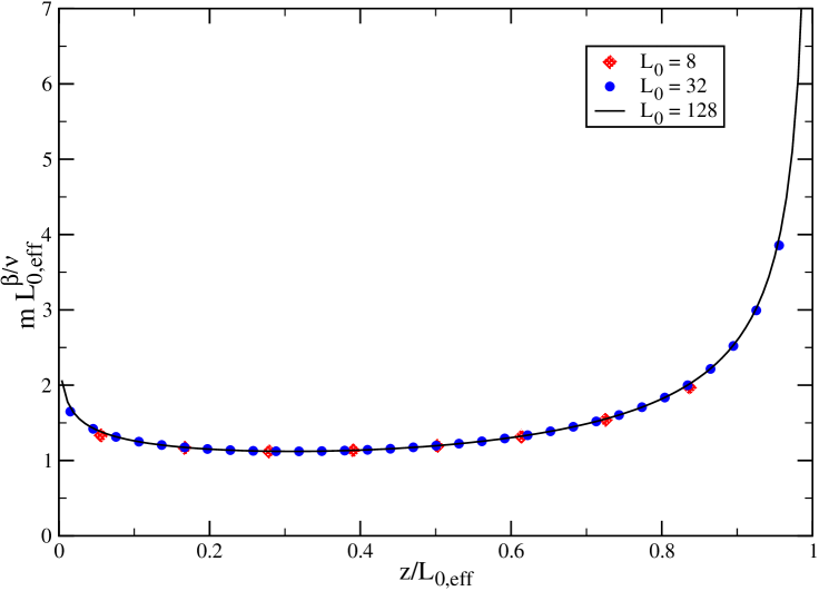
Figure 2: We plot $m(z)L_{0,eff}^{\beta/\nu}$ as a function of $z/L_{0,eff}$, where $z$ is the distance from the boundary with special boundary conditions. The data are taken at the bulk critical point. At the first boundary special boundary conditions and at the second $+$ boundary conditions are applied. We give data for the thicknesses $L_{0}=8$, $32$ and $128$. The line given for $L_{0}=128$ is obtained from a linear interpolation of the data points. We abstained from giving data for more thicknesses to keep the figure readable. Notice that the statistical errors are smaller than the symbols and the line shown. For a detailed discussion see the text. Colour online.

We see that the data for the three different thicknesses fall nicely on top of each other. The same holds for thicknesses not plotted here. Therefore the curve obtained from $L_{0}=128$ should be a good approximation of the universal scaling function $\psi(z/L_{0})$. We observe that, as discussed above, for small $z$ the magnetisation is indeed decreasing with increasing $z$. At $z/L_{0}\approx 0.31$ a very shallow minimum is reached.

VI Summary and Conclusions

In this work we have studied the special point in the phase diagram of a semi-infinite system. We have accurately estimated the surface RG-exponents $y_{t_{1}}$ and $y_{h_{1}}$ that govern, along with the bulk RG-exponents $y_{t}$ and $y_{h}$, the behavior of surface quantities at the special point. To this end, we have simulated the improved Blume-Capel model with two different surface interactions and the spin-1/2 Ising model on the simple cubic lattice. We have determined the surface RG-exponents from a finite size scaling analysis at the special point. In the presence of surfaces typically corrections $\propto L_{0}^{-1}$ appear, where $L_{0}$ is the linear extension of the finite system. Fitting data it is difficult to disentangle these from the leading bulk corrections $\propto L_{0}^{-\omega}$, where $\omega=0.832(6)$ mycritical . Therefore it is helpful that in the improved Blume-Capel model the amplitude of the leading correction to scaling vanishes.

In table 14 we compare our results with those obtained in previous Monte Carlo (MC) studies and computed by field theoretic methods. In previous MC studies only the spin-1/2 Ising model on the simple cubic lattice had been simulated. Only in ref. DeBlNi05 results for the RG-exponents are quoted. However all authors give results for the exponents $\beta_{1}$ and most for $\Phi$. In table 14 we have converted these estimates by using the scaling relations $\beta_{1}=\nu(2-y_{h_{1}})$ and $\Phi=\nu y_{t_{1}}$, where we have used $\nu=0.63002$. In the case of $y_{h_{1}}$ we observe that the estimates of refs. RuWa95 ; DeBlNi05 deviate by $9$ and $6.6$ times the combined error from our result. Notice that such deviations can be caused by corrections that are not taken into account in the ansatz. For a general discussion of this problem see section II.3. The fits performed in ref. DeBlNi05 are in particular prone to this problem, since in the ansatz corrections $\propto L_{0}^{-3}$ are included while e.g. corrections $\propto L_{0}^{-2\omega}$ are missing. In the present work, we tried to estimate such systematical errors by comparing the results obtained by fitting with ansaetze of a varying number of correction terms. In the case of $y_{t_{1}}$ we see a quite good agreement with the results of refs. RuDuWaWu93 ; DeBlNi05 . In contrast, the estimates of refs. BiLa84 ; LaBi90 ; VeRoFa92 are clearly larger than ours.

The surface critical exponents for the special point have been computed up to second order in the $\epsilon$-expansion. Direct results have been obtained for the exponents $\eta_{||}$ Reeve and $\Phi$ DiDi81b . Starting from these two exponents and the bulk exponents, the remaining ones can be computed by using scaling relations. Naively inserting $\epsilon=1$ one gets $\eta_{||}=-0.30$ and $\Phi=0.68$ for three dimensions; see table VI of ref. Diehl86 . In table 14 we give $y_{h_{1}}=(d-\eta_{||})/2$ and $y_{t_{1}}=\Phi/\nu$, where we have used $\nu=0.63002$. The result for $y_{h_{1}}$ is in quite good agreement with those from Monte Carlo simulations. In contrast, the estimate for $y_{t_{1}}$ is by far too large. The authors of ref. DiSh98 have pointed out that by resummation of the series, e.g. by Padé approximants this discrepancy can be resolved. The authors of ref. DiSh98 have computed the surface exponents in a two-loop calculation in three-dimensions fixed. The numerical estimates quoted by the authors are obtained by using Padé approximants. The numbers given in table 14 are again obtained by using $y_{h_{1}}=(d-\eta_{||})/2$ and $y_{t_{1}}=\Phi/\nu$, where $\nu=0.63002$. The results for $y_{h_{1}}$ and in particular for $y_{t_{1}}$ deviate clearly from those obtained from Monte Carlo simulations.

Table 14: Results for the surface RG-exponents of the special phase transition in the three-dimensional Ising bulk universality class.

Ref.	year	Method	$y_{h_{1}}$	$y_{t_{1}}$
BiLa84	1984	MC	1.72(4)	0.89(6)
LaBi90	1990	MC	1.71(3)	0.94(6)
VeRoFa92	1992	MC	1.65	1.17
RuDuWaWu93	1992	MC	1.624(8)	0.732(24)
RuWa95	1995	MC	1.623(2)
SePl98	1998	MC	1.635(16)
DeBlNi05	2005	MC	1.636(1)	0.715(1)
this work	2011	MC	1.6465(6)	0.718(2)
Reeve ; DiDi81b ; Diehl86	1981	$\epsilon$-exp, naive	1.65	1.08
DiDi81b ; DiSh98	1998	$\epsilon$-exp, resummed		0.752
DiSh98	1994	3D-exp, resummed	1.583	0.856

In addition to the estimates of the RG-exponents, our finite size analysis provides us with accurate estimates of the surface coupling $\bar{\beta}_{1,sp}$ at the special point for the three models that we have simulated. These estimates can be used in future studies of thin films. In particular, we intend to study the thermodynamic Casimir force in thin films in the neighborhood of the special point.

Furthermore we have studied the behavior of the surface transition in the neighborhood of the special point. Our numerical results follow the theoretical expectations. However the special point cannot be located accurately with such an approach.

Finally we have simulated a film with symmetry breaking boundary conditions at one surface and special boundary conditions at the other. The behavior of the magnetisation at the surface with special boundary conditions follows a power law. Its exponent can be expressed in terms of the RG-exponent $y_{h_{1}}$. The analysis of the data fully confirms our estimate of $y_{h_{1}}$ given in table 14. The magnetisation profile follows a universal function. This theoretical expectation is fully confirmed by the nice collapse of data that we observe for a large range of thicknesses $L_{0}$ of the film. An interesting feature of the magnetisation profile is that at the surface with special boundary conditions, which do not break the symmetry, the magnetisation is decreasing with increasing distance from the surface.

VII Acknowledgements

This work was supported by the DFG under the grant No HA 3150/2-2.

References

- (1) K. Binder, “Critical Behaviour at Surfaces” in Phase Transitions and Critical Phenomena, Vol. 8, eds. C. Domb and J. L. Lebowitz, (Academic Press, 1983)
- (2) H. W. Diehl, Field-theoretical Approach to Critical Behaviour at Surfaces in Phase Transitions and Critical Phenomena, edited by C. Domb and J.L. Lebowitz, Vol. 10 (Academic, London 1986) p. 76.
- (3) H. W. Diehl, Int. J. Mod. Phys. B 11, 3503 (1997) [arXiv:cond-mat/9610143]
- (4) M. N. Barber, “Finite-size Scaling” in Phase Transitions and Critical Phenomena, Vol. 8, eds. C. Domb and J. L. Lebowitz, (Academic Press, 1983)
- (5) M. Hasenbusch, Phys. Rev. B 82, 174433 (2010) [arXiv:1004.4486]
- (6) Y. Deng and H. W. J. Blöte, Phys. Rev. E 70, 046111 (2004).
- (7) Y. Deng and H. W. J. Blöte, Phys. Rev. E 68, 036125 (2003)
- (8) C. J. Silva, A. A. Caparica, and J. A. Plascak, Phys. Rev. E 73, 036702 (2006).
- (9) M. Hasenbusch, Physica A 197, 423 (1993).
- (10) M. Campostrini, M. Hasenbusch, A. Pelissetto, and E. Vicari, Phys. Rev. B 74, 144506 (2006) [arXiv:cond-mat/0605083]
- (11) R. Guida, J. Zinn-Justin, J. Phys. A 31, 8103 (1998)
- (12) K. E. Newman and E. K. Riedel, Phys. Rev. B 30, 6615 (1984)
- (13) M. Campostrini, A. Pelissetto, P. Rossi, and E. Vicari, Phys. Rev. E 60, 3526 (1999)
- (14) F. J. Wegner J. Math. Phys. 10, 2259 (1971)
- (15) U. Wolff, Phys. Rev. Lett. 62, 361 (1989).
- (16) M. Hasenbusch, K. Pinn and S. Vinti, Phys. Rev. B 59, 11471 (1999)
- (17) M. Saito and M. Matsumoto, “SIMD-oriented Fast Mersenne Twister: a 128-bit Pseudorandom Number Generator”, in Monte Carlo and Quasi-Monte Carlo Methods 2006, edited by A. Keller, S. Heinrich, H. Niederreiter, (Springer, 2008); M. Saito, Masters thesis, Math. Dept., Graduate School of schience, Hiroshima University, 2007. The source code of the program is provided at “http://www.math.sci.hiroshima-u.ac.jp/m-mat/MT/SFMT/index.html”
- (18) K. Binder and D. P. Landau, Phys. Rev. Lett. 52, 318 (1984)
- (19) D. P. Landau and K. Binder, Phys. Rev. B 41, 4633 (1990)
- (20) C. Ruge, S. Dunkelmann and F. Wagner, Phys. Rev. Lett. 69 (1992) 2465 C. Ruge, S. Dunkelmann, F. Wagner, and J. Wulf, J. Stat. Phys. 73, 293 (1993).
- (21) Y. Deng, H. W. J. Blöte, and M. P. Nightingale, Phys. Rev. E 72, 016128 (2005) [arXiv:cond-mat/0504173].
- (22) M. Caselle and M. Hasenbusch, Nucl. Phys. B 470, 435 (1996) [arXiv:hep-lat/9511015]
- (23) M. Caselle, M.Hasenbusch, A. Pelissetto, and E. Vicari, J. Phys. A 35, 4861 (2002) [arXiv:cond-mat/0106372]
- (24) M. Hasenbusch, Phys. Rev. B 83, 134425 (2011) [arXiv:1012.4986]
- (25) C. Ruge and F. Wagner, Phys. Rev. B 52, 4209 (1995)
- (26) M. Pleimling and W. Selke, Eur. Phys. J. B 1, 385 (1998)
- (27) M. Vendruscolo, M. Rovere, and A. Fasolino, Europhys. Lett. 20, 547 (1992)
- (28) J. S. Reeve, Phys. Lett. A 81, 237 (1981)
- (29) H. W. Diehl and S. Dietrich, Phys. Rev. B 24, 2878 (1981); H. W. Diehl and S. Dietrich, Z. Phys. B 50, 117 (1983)
- (30) H. W. Diehl and M. Shpot, Phys. Rev. Lett. 73, 3431 (1994); H. W. Diehl and M. Shpot, Nucl. Phys. B 528, 595 (1998)