Effect of Electron-electron Interaction on Surface Transport in Three-Dimensional Topological Insulators

Abstract

We study the effect of electron-electron interaction on the surface resistivity of three-dimensional (3D) topological insulators. In the absence of umklapp scattering, the existence of the Fermi-liquid ($T^{2}$) term in resistivity of a two-dimensional (2D) metal depends on the Fermi surface geometry, in particular, on whether it is convex or concave. On doping, the Fermi surface of 2D metallic surface states in 3D topological insulators of the Bi₂Te₃ family changes its shape from convex to concave due to hexagonal warping, while still being too small to allow for umklapp scattering. We show that the $T^{2}$ term in the resistivity is present only in the concave regime and demonstrate that the resistivity obeys a universal scaling form valid for an arbitrary 2D Fermi surface near a convex/concave transition.

Topological insulators (TI) are characterized by a gapped bulk spectrum with conducting surface states extending across the entire gap. The surface states contain an odd number of Dirac cones and are protected against any perturbation that preserves time-reversal symmetry general . A wide variety of interesting physics resulting from these surface states is expected to be observed ranging from Majorana fermions majorana to magnetic monopoles monopole . Although photoemission and tunneling microscopy arpes_stm have convincingly established the presence of such surface states in these materials, signatures of these states in transport measurements are more difficult to observe, mainly because of strong conduction in the bulk bulk . With recent experimental progress, however, in the ability to tune the number of surface charge carriers tune , it is now possible to see more clearly evidence of surface transport. In light of this progress, it is timely to ask what is the effect of the electron-electron (e-e) interaction on surface transport. Indeed, including e-e interaction is crucial for explaining the observed field and temperature dependences in quantum magnetotransport magres . In this Letter, we address the manifestation of the e-e interaction in semiclassical transport within a model of a two-dimensional Fermi liquid relevant for surface states doped away from the Dirac point.

An archetypal signature of the Fermi-liquid behavior in metals is the $T^{2}$ dependence of the resistivity ($\rho$). With an exception of compensated semi-metals baber:37 , this dependence in clean conductors arises due to a special type of scattering processes–“umklapps” peierls:29 ; landau:36 – in which the total momentum of an electron pair is changed by an integer multiple of the reciprocal lattice vector. Umklapps are possible if certain conditions are met, namely, if the Fermi surface (FS) is large enough (the band is more than quarter full) and if the matrix element of the interaction has sufficient weight at large momentum transfers. Otherwise, the umklapp contribution to the resistivity is suppressed. In this case, the $T^{2}$ contribution to $\rho$ may still occur due to the combined effect of the momentum-conserving (“normal”) interaction among electrons on a lattice and electron-impurity (e-i) scattering. Whether this really happens, turns out to depend crucially on the dimensionality. While the $T^{2}$ term is allowed for an anisotropic FS with a non-parabolic spectrum in three dimensions (3D), the conditions in two dimensions (2D) are much more stringent gurzhi . In particular, a $T^{2}$ term occurs in 2D only if the FS is either concave or multiply-connected; otherwise, the leading e-e contribution scales as $T^{4}$ maslov . Likewise, the frequency dependence of the ac resistivity scales as $\Omega^{4}$ instead of $\Omega^{2}$ rosch . The reason for such a behavior is that the $T^{2}$ ($\Omega^{2}$) term arises from electrons confined to the FS contour. For a convex and singly-connected contour, the momentum and energy conservations are similar to the 1D case, where no relaxation is possible.

We propose the surface state of a 3D TI as a testing ground for the theoretical results outlined above. Photoemission shows that the surface states of the Se, Te based compounds (Bi₂Te₃, Bi₂Se₃, and Sb₂Te₃) have a small, singly-connected FS at the center of the Brilllouin zone (BZ). Following Fu fu , the electronic dispersion in these systems can be described by

$$\epsilon_{\mathbf{k}}^{\pm}=\pm\sqrt{v^{2}k^{2}+\lambda^{2}k^{6}\mathrm{cos}^{2}(3\theta)},$$ (1)

where $\theta$ is the azimuthal angle, $v$ is the Dirac velocity, and $\lambda$ is a constant. Corresponding isoenergetic contours are presented in Fig. 1. As the Fermi energy increases, the FS changes rapidly from a circle to a hexagon and then to a hexagram. At some critical value of the Fermi energy $\epsilon_{F}=\epsilon_{c}$ ($=0.16$ eV for Bi₂Te₃, for example fu ), the shape changes from convex to concave. Theory rosch ; maslov predicts, therefore, that the e-e contribution to the resistivity scales as $\max\{T^{4},\Omega^{4}\}$ on the convex side and as $\max\{T^{2},\Omega^{2}\}$ on the concave side. The main result of this Letter is that, near the convex/concave transition, the resistivity obeys a universal scaling form

$$\rho=\rho_{0}+A\left(\frac{\Delta}{\epsilon_{F}}\right)^{9/2}\Theta(\Delta)T^{2}+BT^{4},$$ (2)

where $\rho_{0}$ is the residual resistivity, $\Delta=\epsilon_{F}-\epsilon_{c}$, $\theta(x)$ is the step function, and $A$, $B$ are material-dependent parameters.

The exponents of $2$, $4$, and $9/2$ in Eq. (2) are universal, i.e., they are the same for an arbitrary 2D Fermi surface with a non-quadratic energy spectrum near a convex/concave transition. We emphasize, however, that the surface states of 3D TIs present a unique case of a small yet strongly warped 2D FS, where the predicted effects can be seen best. The drawback of 3D TIs is that they have a large background dielectric constant ($\epsilon\sim 29-85$ dielectric ), and hence, the electron-phonon (e-ph) interaction is expected to dominate the $T$-dependence of the resistivity down to very low $T$eph . This drawback can be circumvented by measuring the frequency dependence of the optical conductivity at frequencies above the Bloch-Gruneisen frequency, where the e-e contribution dominates over the e-ph one ephsaturate .

As in Ref. maslov , we adopt an approach based on the semiclassical Boltzmann equation (BE) comment2 and neglect quantum corrections to the conductivity. For simplicity, the e-i interaction is accounted for within the $1/\tau$ approximation. First, we consider the dc case ($\Omega=0$). For low enough $T$, when $\tau_{ee}\gg\tau_{ei}$, we solve the BE to leading order in the e-e interaction and obtain the correction to the residual conductivity as

$$\delta\sigma_{jj}= - \frac{e^{2}\tau_{i}^{2}}{2T}\int\frac{d^{2}q}{(2\pi)^{2}}\int\int\int d\omega d\epsilon_{\mathbf{k}}d\epsilon_{\mathbf{p}}\oint\oint\frac{da_{\mathbf{k}}}{v_{\mathbf{k}}}\frac{da_{\mathbf{p}}}{v_{\mathbf{p}}}$$

$$\times |M_{\mathbf{k},\mathbf{p}}(\mathbf{q})|^{2}(\Delta\mathbf{v}_{j})^{2}n(\epsilon_{\mathbf{k}})n(\epsilon_{\mathbf{p}})[1-n(\epsilon_{\mathbf{k}}-\omega)]$$

$$\times [1-n(\epsilon_{\mathbf{p}}+\omega)]\delta(\epsilon_{\mathbf{k}}-\epsilon_{\mathbf{k}-\mathbf{q}}-\omega)\delta(\epsilon_{\mathbf{p}}-\epsilon_{\mathbf{p}+\mathbf{q}}+\omega).$$

Here, $\tau_{i}$ is the mean free time due to impurity scattering, $\mathbf{q}$ and $\omega$ are the momentum and energy transfers, $\Delta\mathbf{v}=\mathbf{v}_{\mathbf{k}}+\mathbf{v}_{\mathbf{p}}-\mathbf{v}_{\mathbf{k}-\mathbf{q}}-\mathbf{v}_{\mathbf{p}+\mathbf{q}}$, $da_{\mathbf{l}}$ is the FS element, $n(\epsilon_{\bf l})=\left(\exp\left(\epsilon_{\bf l}/T\right)+1\right)^{-1}$, and $M_{\mathbf{k},\mathbf{p}}(\mathbf{q})$ is the matrix element of the e-e interaction. To obtain the lowest in $T$ term in $\delta\sigma_{jj}$, we project electrons onto the FS, which amounts to neglecting $\omega$ in the arguments of the $\delta$ functions. Since the typical values of $\epsilon_{\bf k,p}$ and $\omega$ are of order $T$, while the typical values of other variables are $T$ independent, $\delta\sigma_{jj}$ scales as $T^{2}$, which is the expected Fermi-liquid behavior. However, whether the prefactor of the $T^{2}$ term is non-zero depends on whether $\Delta{\bf v}$ is non-zero for all ${\bf k}$, ${\bf p}$, and ${\bf q}$ satisfying energy conservation. On relabeling $\mathbf{p}$ to $-\tilde{\mathbf{p}}$ and invoking time-reversal symmetry, the arguments of both $\delta$ functions become the same. The problem of finding the allowed initial states ${\bf k}$ and ${\bf p}$ at fixed ${\bf q}$ now reduces to finding the solutions of the equation $\epsilon_{\mathbf{k}}=\epsilon_{\mathbf{k}-\mathbf{q}}$ (and the same for $\mathbf{k}\to\tilde{\mathbf{p}}$). Geometrically, this is equivalent to shifting the FS by a vector $\mathbf{q}$ and finding $\mathbf{k}$ and $\tilde{\mathbf{p}}$ as the points where the original and shifted FSs intersect.

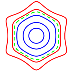
Figure 1: (color online). Isoenergetic contours for the spectrum in Eq. (1). The dashed line corresponds to the critical energy for the convex/concave transition.

Consider first the case $\epsilon_{F}<\epsilon_{c}$, when the FS is convex. As shown in Fig. 2(a), there are only two points of intersection. If $\mathbf{k}$ is one of these intersection points then, by symmetry, the other point is $-\mathbf{k}+\mathbf{q}$. Since solutions for $\tilde{\mathbf{p}}$ must belong to the same set $\{\mathbf{k},-\mathbf{k}+\mathbf{q}\}$, the scattering process either occurs in the Cooper channel ($\{\mathbf{k},-\mathbf{k}\}\to\{\mathbf{k}-\mathbf{q},-\mathbf{k}+\mathbf{q}\}$) or corresponds to swapping of initial momenta ($\{\mathbf{k},\mathbf{k}-\mathbf{q}\}\to\{\mathbf{k}-\mathbf{q},\mathbf{k}\}$). In both cases, $\Delta{\bf v}=0$, and thus the $T^{2}$ correction to the conductivity vanishes. The first nonvanishing term in this case is $T^{4}$, which can be obtained from Eq. (Effect of Electron-electron Interaction on Surface Transport in Three-Dimensional Topological Insulators) by expanding the product of the $\delta$ functions to second order in $\omega$. On the other hand, if the FS is concave ($\epsilon_{F}>\epsilon_{c}$), there are six possible points of intersection yielding six solutions for each $\mathbf{k}$ and $\tilde{\mathbf{p}}$ [cf. Fig. 2(b)]. The total set of thirty six pairs for $\{\mathbf{k},\tilde{\mathbf{p}}\}$ contains processes other than Cooper channel and swapping, and $\Delta\mathbf{v}$ is non-zero for these processes.

The analysis presented above is valid either well below or well above the convex/concave transition, i.e., when $|\Delta|\sim\epsilon_{F}$. We now turn to the vicinity of the transition, when $|\Delta|\ll\epsilon_{F}$. First, we focus on the most interesting case of $\Delta\gg T$, when the isoenergetic contours near the Fermi energy are concave, and then discuss the case of $|\Delta|\lesssim T$, when both convex and concave contours near the FS are thermally populated. Near the transition, several quantities in Eq. (Effect of Electron-electron Interaction on Surface Transport in Three-Dimensional Topological Insulators) exhibit a critical dependence on $\Delta$. First, it is $\Delta\mathbf{v}$ which is zero on the convex side and non-zero on the concave side. Additionally, there are two other quantities which also show a critical behavior. As Figs. 2(c) and 2(d) illustrate, even if the FS is concave, it has more than two self-intersection points only if it is shifted along one of the special directions and the magnitude of the shift is sufficiently small. [These special directions are high-symmetry axes that intersect the FS at points with positive curvature, as in Fig. 2(b).] Therefore, the width of the angular interval near a special direction ($\Delta\theta_{\mathbf{q}}$) and the maximum value of $q$ ($q_{\max}$ also depend on $\Delta$ in a critical manner. Approximating $\int d^{2}q$ by $\Delta\theta_{\mathbf{q}}q_{\max}^{2}$, resolving the $\delta$ functions, and integrating over all energies, we obtain

$$\delta\sigma_{jj} = -\frac{e^{2}\tau_{i}^{2}T^{2}}{12}\sum_{l,m}\Delta\theta_{\mathbf{q}}|M_{\mathbf{k}_{l},\mathbf{p}_{m}}(\mathbf{q}_{\max})|^{2}$$ (4)

$$\times [\Delta\mathbf{v}_{j}]_{lm}^{2}\frac{k_{l}}{\mathbf{v}_{\mathbf{k}_{l}}\cdot\hat{\mathbf{k}}_{l}}\frac{p_{m}}{\mathbf{v}_{\mathbf{p}_{m}}\cdot\hat{\mathbf{p}}_{m}}\frac{1}{|\mathbf{v}^{{}^{\prime}}_{\mathbf{k}_{l}}\cdot\hat{\mathbf{q}}|}\frac{1}{|\mathbf{v}^{{}^{\prime}}_{\mathbf{p}_{m}}\cdot\hat{\mathbf{q}}|},$$

where the sum runs over all intersection points, the prime denotes a derivative with respect to the azimuthal angle, and $\hat{\mathbf{l}}\equiv\mathbf{l}/|\mathbf{l}|$. Notice that although a factor of $q^{2}_{\max}$ from the phase space of integration cancels with the same factor from the $\delta$ functions, it will reappear in the calculation of $\Delta\mathbf{v}_{j}$. We are now going to show that

$$\Delta\theta_{\mathbf{q}}\propto\Delta^{3/2},q_{\max}\propto\Delta^{1/2},\;\mathrm{and}\;\Delta\mathbf{v}_{j}\propto\Delta^{3/2}.$$ (5)

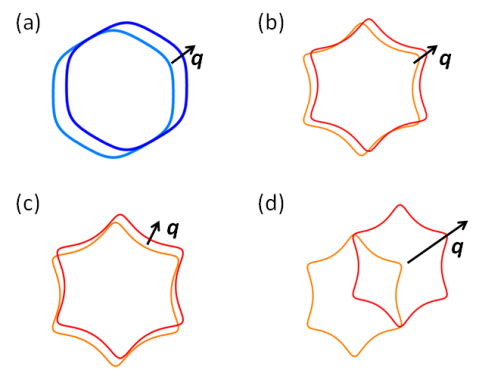
Figure 2: (color online). (a) A convex contour has no more than two self-intersection points. (b) For q along a special direction, a concave contour has the maximum number (6 for a sixfold-symmetric FS) of self-intersection points. (c) Even in the concave case, the number of self-intersection points is less than the maximal number allowed by symmetry, if $\mathbf{q}$ is not along a special direction. (d) For $q$ larger than a critical value, the number of the self-intersection points is less than the maximum number allowed by symmetry.

We begin with $\Delta\theta_{\mathbf{q}}$. Under an assumption (to be justified later) of small $q$, the equation $\epsilon_{\mathbf{k}}-\epsilon_{\mathbf{k}-\mathbf{q}}=0$ reduces to $\mathbf{v}_{\mathbf{k}}\cdot\mathbf{q}=0$, which implies that $\mathbf{q}$ is a tangent to the FS at the intersection points [cf. Fig. 3(a)]. Defining $\theta^{*}$ as an angle between the normal to the FS at any given point and $\mathbf{q}$, we plot $\theta^{*}$as a function of the azimuthal angle $\theta$. Figure 3(b) clearly demonstrates a distinguishing feature between the convex and concave contours: $\theta^{*}(\theta)$ is monotonic for the former and non-monotonic for the latter. The non-monotonic part is centered around certain invariant points, i.e., common points for all contours. The oscillations reflect the rotational symmetry–sixfold in our case–of the FS. From symmetry, if $\theta$ is a solution, so is $\theta+\pi$; we thus consider only the domain $\theta\in[0,\pi]$. We now need to find the angular interval of $\mathbf{q}$ about a special direction in which the equation $\theta^{*}=\theta_{\mathbf{q}}+\pi/2$ has three roots; the $T^{2}$ term is non-zero only in this case. Since there is a one-to-one correspondence between the angles $\theta^{*}$ and $\theta_{\mathbf{q}}$, we can find the corresponding interval $\Delta\theta^{*}$ instead of $\Delta\theta_{\mathbf{q}}$. Clearly, the regions on the curve where it is non-monotonic are responsible for the multiple roots light . Redefining variables $\theta$ and $\theta^{*}$ as measured from the invariant points, the non-monotonic part of the curve can be conjectured to obey a cubic equation [cf. Fig. 3(c)]:

$$\theta^{*}=b\theta^{3}-a(\Delta)\theta,$$ (6)

where $a(\Delta)\propto\Delta$ and $b>0$ is a constant. Indeed, we need at least a cubic equation to provide for three real roots; whether there is one or three roots depends on the sign of $a(\Delta)$ which must be negative/positive in the convex/concave regimes, correspondingly. For the model spectrum of Eq. (1), we find $b=2$ and $a(\Delta)=\frac{16}{9}\sqrt{\frac{7}{6^{1/2}}(\frac{\lambda}{v^{3}})}\Delta$. The quantity $\Delta\theta^{*}$ is the vertical distance between the maximum and minimum of this curve which, according to Eq. (6) scales as $\Delta^{3/2}$.

Next in line is $\Delta\mathbf{v}_{j}$, which we expand in small $q$ as $\Delta\mathbf{v}_{j}\approx[\frac{\partial}{\partial k_{j}}(\mathbf{q}\cdot\mathbf{v})]|_{\mathbf{k}_{2}}-[\frac{\partial}{\partial k_{j}}(\mathbf{q}\cdot\mathbf{v})]|_{\mathbf{k}_{1}}=[\frac{\partial}{\partial k_{j}}(\mathbf{q}\cdot\mathbf{v})]|^{\mathbf{k}_{2}}_{\mathbf{k}_{1}}$, where $\mathbf{k}_{2}$ and $\mathbf{k}_{1}$ are any two solutions of the equation $\mathbf{q}\cdot\mathbf{v}_{\mathbf{k}}=0$. Referring to the geometry of Fig. 3(d), we find $\Delta\mathbf{v}_{j}\propto q[\frac{\partial}{\partial\theta}(\theta^{*})]|^{\theta_{2}}_{\theta_{1}}$, where use of Eq. (6) yields $\Delta\mathbf{v}_{j}\propto q\Delta\approx q_{\max}\Delta$.

Finally, to find $q_{\max}$, we relax the assumption of small $q$ and solve the equation $\epsilon_{\mathbf{k}-\mathbf{q}}=\epsilon_{\mathbf{q}}$ for arbitrary $q$. It is easier to do this by casting Eq. (6) into an equation for the contour in terms of local cartesian coordinates. To this effect, we approximate $\theta^{*}\approx\mathrm{tan}\theta^{*}\approx dk_{y}/dk_{x}$ and $\theta\approx\mathrm{tan}\theta\approx-k_{x}/k_{F}^{0}$, with $k_{F}^{0}$ being the Fermi momentum at the invariant point [cf. Fig. 3(d)] and substitute into Eq. (6) to get the following contour equation: $k_{y}=-bk_{x}^{4}/4+a(\Delta)k_{x}^{2}/2$, where $k_{x,y}$ are the momenta measured from the invariant points and normalized by $k_{F}^{0}$. Using this expression to solve for the roots of $\epsilon_{\mathbf{k}-\mathbf{q}}=\epsilon_{\mathbf{q}}$ one arrives at a cubic equation in $k_{x}$, which has three distinct real roots if $q\leq 2\sqrt{a(\Delta)/b}$. This means that $q_{\max}\propto\Delta^{1/2}$ (and thus $\Delta{\bf v}_{j}\propto\Delta^{3/2}$). This, in hindsight, validates the assumption of small $q$.

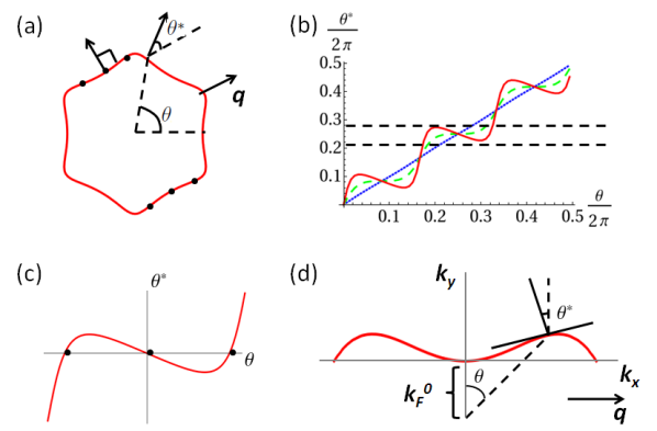
Figure 3: (color online). (a) For small $q$, points where the normal to the FS is perpendicular to $\mathbf{q}$ are the points of self-intersection (black dots). (b) $\theta^{*}$ vs $\theta$ [as defined in panel (a)]. Dotted: $\epsilon<\epsilon_{c}$; dashed: $\epsilon=\epsilon_{c}$; solid: $\epsilon>\epsilon_{c}$. (c) A zoom of the non-monotonic part of the graph in panel (b). (d) A portion of the FS contour showing the geometrical construction for the derivation of the equation for the contour.

Collecting all the terms together, the resultant energy dependence of the critical terms is $\Delta\theta_{\mathbf{q}}[\Delta\mathbf{v}_{j}]^{2}\propto\Delta^{9/2}$. which leads to the scaling form of the prefactor of the $T^{2}$ term in Eq. (2). The Cooper and swapping channels of scattering always contribute a $T^{4}$ term to the resistivity, and the second term in Eq. (2) accounts for this contribution. A crossover between the $T^{4}$ and $T^{2}$ behaviors occurs at $T\sim\epsilon_{F}(\Delta/\epsilon_{F})^{9/4}\ll\epsilon_{F}$. A large value of the exponent ($9/2$) indicates that one needs to go sufficiently high above the convex/concave transition in order to see the $T^{2}$ term.

Now we return to the range of energies $\Delta\lesssim T$, when both convex and concave contours are populated. Instead of a $\Delta^{9/2}$ factor, we get a factor of $T^{9/2}$, leading to a $T^{13/2}$ term in $\rho$. This term, however, is subleading to the $T^{4}$ one. Therefore, we conclude that Eq. (2) describes the leading $T$-dependence of the resistivity in all possible situations near the transition.

Next, we discuss the feasibility of observing these predictions in an experiment. First of all, one needs to ask if the e-ph contribution to the resistivity masks the e-e one. In general, the e-ph contribution, which scales as $T^{5}$ at $T<T_{BG}$, where $T_{BG}$ is Bloch-Gruneisen temperature ($\approx 10K$ for Bi₂Te₃ eph ), is expected to be outweighed by the $T^{2}$ (or even $T^{4}$) one from the e-e interaction. However, the e-e coupling may be substantially reduced due to high background polarizability of TI materials. Indeed, comparing the scattering time of e-ph interaction, calculated in Ref. eph , with that of the e-e interaction, we find that the $T^{5}$ term dominates over the $T^{2}$ one down to a few mK. Even with some uncertainty in the estimate of the e-ph time related to screening of this interaction by free electrons, the detection of the $T^{2}$ term in a dc measurement seems to be difficult. Instead, as an alternate route to test our predictions, we suggest measuring the optical conductivity as a function of the frequency $\Omega$. Indeed, the crossover between the $T^{4}$ and $T^{2}$ forms of the dc resistivity is completely analogous to the that between the $\Omega^{4}$ and $\Omega^{2}$ forms of the optical scattering rate $\Gamma(\Omega)\equiv(\omega^{*}_{p})^{2}\mathrm{Re}\rho(\Omega)$ rosch . It can be readily shown that the effective plasma frequency $\omega_{p}^{*}$ contains the same integrals as in Eq. (Effect of Electron-electron Interaction on Surface Transport in Three-Dimensional Topological Insulators) rosch ; plasma . Therefore, all the foregoing conclusions on the temperature dependence at different values of $\epsilon_{F}$ carry over to the frequency dependence. The advantage of an optical measurement is that the e-ph part of $\Gamma(\Omega)$ saturates ephsaturate for $T_{BG}\ll\Omega\ll\epsilon_{F}$, while the e-e part continues to grow either as $\Omega^{2}$ or $\Omega^{4}$, depending on the sign of $\Delta$. This advantage was used in the past to detect the e-e contribution to $\Gamma(\Omega)$ in noble metals ephsaturate , and we propose to apply the same technique to TIs.

- (1) O. A. Pankratov, S. V. Pakhomov, and B. A. Volkov, Solid State Commun. 61, 93 (1987); C. L. Kane and E. J. Mele, Phys. Rev. Lett. 95, 226801 (2005); L. Fu and C. L. Kane, Phys. Rev. B 76, 045302 (2007); König, et al., Science 318, 766 (2007); D. Hsieh, et al., Nature (London) 452, 970 (2008); Y. Xia, et al., Nat. Phys. 5, 398 (2009); H. Zhang, et al., Nat. Phys. 5, 438 (2009).
- (2) L. Fu and C. L. Kane, Phys. Rev. Lett. 100, 096407 (2008).
- (3) X. Qi, et al., Science 323, 1184 (2009).
- (4) D. Hsieh, et al., Science 323, 919 (2009); Y. L. Chen, et al., Science 325, 178 (2009); Z. Alpichshev, et al., Phys. Rev. Lett. 104, 016401 (2010); P. Cheng, et al., Phys. Rev. Lett. 105, 076801 (2010); T. Hanaguri, et al., Phys. Rev. B 82, 081305 (2010).
- (5) J. G. Checkelsky, et al., Phys. Rev. Lett. 103, 246601 (2009); D. X. Qu, et al., Science 329, 821 (2010); N. P. Butch, et al., Phys. Rev. B 81, 241301 (2010).
- (6) J. G. Analytis, et al., Nat. Phys. 6, 960 (2010); Y. S. Hor, et al., arXiv:1006.0317 (2010); H. Steinberg, et al., Nano Lett. 10, 5032 (2010).
- (7) J. Wang, et al., arXiv:1012.0271v2 (2011).
- (8) W. G. Baber, Proc. R. Soc. London Ser. A156, 383 (1937).
- (9) R. Peierls, Ann. Phys. 3, 1055 (1929).
- (10) L. D. Landau and I. J. Pomeranchuk, Phys. Z. Sowjetunion 10, 649 (1936); Zh. Eksp. Teor. Fiz. 7, 379 (1937).
- (11) R. N. Gurzhi, A. N. Kalinenko, and A. I. Kopeliovich, Phys. Rev. B 52, 4744 (1995).
- (12) D. L. Maslov, V. I. Yudson, and A. V. Chubukov, Phys. Rev. Lett. 106, 106403 (2011).
- (13) A. Rosch and P. C. Howell, Phys. Rev. B72, 104510 (2005); A. Rosch, Ann. Phys. 15, 526 (2006).
- (14) L. Fu, Phys. Rev. Lett. 103, 266801 (2009).
- (15) W. Richter, H. Köhler, and C.R. Becker, Phys. Stat. Sol. (b) 84, 619 (1977).
- (16) S. Giraud and R. Egger, arXiv: 1103.0178v1 (2011).
- (17) See V. F. Gantmakher and Y. B. Levinson, Scattering in metals and semiconductors (North-Holland, 1987) and references therein.
- (18) Although we use a scalar BE instead of a spinor one suitable for helical states, it does not affect any of our conclusions. Away from the Dirac point, the effect of the phase factors in the spinor wavefunctions is only to suppress backscattering probability of all processes considered.
- (19) In light of this, it is now clear why a convex contour does not allow for more than two solutions and why a concave contour allows for more than two solutions only for special directions of .
- (20) E. G. Mishchenko, M. Y. Reizer, and L. I. Glazman, Phys. Rev. B 69, 195302 (2004).