Vicious accelerating walkers

Abstract

A vicious walker system consists of $N$ random walkers on a line with any two walkers annihilating each other upon meeting. We study a system of $N$ vicious accelerating walkers with the velocity undergoing Gaussian fluctuations, as opposed to the position. We numerically compute the survival probability exponent, $\alpha$, for this system, which characterizes the probability for any two walkers not to meet. For example, for $N=3$, $\alpha=0.71\pm 0.01$. Based on our numerical data, we conjecture that $\frac{1}{8}N(N-1)$ is an upper bound on $\alpha$. We also numerically study $N$ vicious Levy flights and find, for instance, for $N=3$ and a Levy index $\mu=1$ that $\alpha=1.31\pm 0.03$. Vicious accelerating walkers relate to no-crossing configurations of semiflexible polymer brushes and may prove relevant for a non-Markovian extension of Dyson’s Brownian motion model.

I Introduction

Consider $N$ random walkers on a line. The only interaction between the walkers is that if any two walkers meet, they annihilate each other, hence these walkers are deemed vicious. This system was introduced by M. E. Fisher in his 1983 Boltzmann Medal lecture and was applied to interfacial wetting in $1+1$ dimensions since the interaction of different interfaces (walkers) drives the wetting transition Fisher ; Fisher.Huse . In addition, the fermionic nature of vicious walkers provides a Coulomb gas description and, thereby, a link with Gaussian random matrices Dyson ; Forrester . More specifically, Baik has proven that a particular limiting conditional distribution of the displacement of the leftmost walker is equivalent to the Tracy-Widom distribution for the Gaussian Orthogonal Ensemble(GOE) Baik . Moreover, vicious walker configurations correspond to directed polymer brushes with the vicious mechanism capturing the non-intersecting property of the polymers Essam . So while the study of vicious walkers has attracted attention from the mathematical physics community, a number of different physical applications also drive its study.

There have been generalizations of vicious walkers to dissimilar walkers Gelfand , walkers with drift Wrinkler , and walkers with external potentials Bray . Here, we introduce a system of $N$ accelerating vicious walkers and study the survival probability, $s(t)$, the probability of having none of the $N$ walkers annihilated up to time $t$. In one-dimension, a randomly accelerating walker, $x(t)$, is defined by

$$\frac{d^{2}x(t)}{dt^{2}}=\eta(t),$$ (1)

where $\eta(t)$ is Gaussian noise with $\langle\eta(t)\rangle=0$ and $\langle\eta(t)\eta(t^{\prime})\rangle=2D\delta(t-t^{\prime})$. The corresponding Fokker-Planck equation is

$$\left[D\frac{\partial^{2}}{\partial v^{2}}-v\frac{\partial}{\partial x}\right]p(x,v,t)=\frac{\partial}{\partial t}p(x,v,t),$$ (2)

where $p(x,v,t)$ is the probability density distribution for a randomly accelerating walker in one-dimension.

A randomly accelerating walker is presumably the simplest non-Markovian stochastic process. Given the fermionic interaction between vicious accelerating walkers, one can explore the possibility of a non-Markovian analogue to the Coulomb gas and, hence, a potentially new class of non-Markovian random matrices. Recently, Fukushima and collaborators have revisited Dyson’s original Brownian motion model for random matrices and found another non-Markovian stochastic process after generalizing the coefficients of the matrices Fukushima . In addition, a randomly accelerating walker appears in the Boltzmann weight of an extensible, semiflexible polymer of length $L$ with non-zero bending energy Burkhardt . For a given displacement vector $\vec{r}(z)$ from some reference point along a contour length, $z$, the Hamiltonian, $H$, is given by

$$H(\vec{r}(z),\vec{u}(z);z)=\frac{\kappa}{2}\int_{0}^{L}{dz}\left(\frac{d^{2}\vec{r}(z)}{dz^{2}}\right)^{2},$$ (3)

where $\vec{u}(z)$ denotes the tangent vector and $\kappa$ characterizes the bending rigidity. Mapping the contour length $z$ to time $t$ and the displacement vector $\vec{r}$ to $\vec{x}(t)$, the equation of motion for this system corresponds to a randomly accelerating walker in the corresponding dimension. Implementing the vicious interaction between $N$ random accelerating walkers, therefore, corresponds to the statistics of non-intersecting semiflexible polymer brushes. In the interest of studying a mixture of flexible and semiflexible polymer brushes, one can also address a mixture of vicious accelerating and random walkers. Please see the appendix for some discussion of $N\leq 3$ vicious mixed walkers system.

II $N\leq 3$ vicious accelerating walkers

We begin by considering $N=2$ vicious accelerating walkers in one-dimension with equal diffusion constants $D_{1}=D_{2}=D$. The two accelerating walkers are governed by the equation,

$$D\left(\frac{\partial^{2}}{\partial v_{1}^{2}}+\frac{\partial^{2}}{\partial v_{2}^{2}}\right)p(x_{1},x_{2},v_{1},v_{2},t)$$

$$-\left(v_{1}\frac{\partial}{\partial x_{1}}+v_{2}\frac{\partial}{\partial x_{2}}\right)p(x_{1},x_{2},v_{1},v_{2},t)=$$

$$\frac{\partial}{\partial t}p(x_{1},x_{2},v_{1},v_{2},t)$$ (4)

with the initial condition, $p(x_{1},x_{2},v_{1},v_{2},t=0)=\delta(x_{1}-x_{1,i})\delta(x_{2}-x_{2,i})\delta(v_{1})\delta(v_{2})$, with $x_{1,i}<x_{2,i}$. In addition, to compute the survival probability, $s(t)$, we implement the boundary condition,

$$p(x_{1}=x_{2},v_{1}>v_{2},t)=0$$ (5)

such that the system “dies” when the two walkers meet in space and have ingoing velocities. Note that the boundary condition in $v$ is redundant since, due to the initial positions, the two walkers cannot meet with a relative outgoing velocity.

We then choose the relative coordinate system to reduce the $N=2$ vicious accelerating walkers to one random accelerating walker in the presence of an absorbing wall. This change of variables takes the form, $x=x_{1}-x_{2}$ and $v=v_{1}-v_{2}$. The Fokker-Planck equation thereby reduces to

$$\left[2D\frac{\partial^{2}}{\partial v^{2}}-v\frac{\partial}{\partial x}\right]p(x,v,t)=\frac{\partial}{\partial t}p(x,v,t),$$ (6)

with the boundary condition, $p(x=0,v>0,t)=0.$

The survival probability for this process is nontrivial in that one cannot invoke the method of images as is done for the ordinary random walker. Using properties of the integral of a Brownian curve, Sinai Sinai proved that the asymptotic survival probability distribution is given by

$$s(t)\sim t^{-1/4}$$ (7)

at long times. Note that the first-passage time distribution, $f(t)$, where the first passage time is defined by the time at which any of the two walkers meet is given by $f(t)=-\frac{ds(t)}{dt}$ such that $f(t)\sim t^{-5/4}$. In general, if the survival probability distribution is given by $s(t)\sim t^{-\alpha}$ at large times, then $f(t)\sim t^{-\beta}$ with $\beta=\alpha+1$.

A heuristic argument, based on Sinai’s approach, for $\alpha=1/4$ was given in Ref. Schwarz . First, a new time counter, $M$, is defined by each “original” time the velocity crosses zero. In other words, the original time is now defined by the distribution of first-passage time of a random walk undergoing a Levy flight with Levy index $\mu=1/2$. Moreover, with this new counting, the position variable is also a Levy flight with Levy index $\mu=1/3$. By invoking the powerful superuniversality of the Sparre-Andersen theorem in one-dimension SparreAndersen ; Feller ; Majumdar , the first passage time distribution for the position in terms of $M$ is the same as for a random walk, i.e. $M^{-3/2}$. To convert back to the original time, one simply needs to compute the integral

$$f(t)\sim\int\frac{1}{M^{\frac{3}{2}}}\frac{M}{t^{\frac{3}{2}}}\exp(-t^{2}/M)dM,$$ (8)

where $\frac{M}{t^{\frac{3}{2}}}\exp(-t^{2}/M)$ is the limiting distribution for the sum of $M$ $\mu=1/2$ Levy variables. We should also mention that Burkhardt Burkhardt made the use of Marshall-Watson functionsMarshall.Watson to solve for the Laplace transform version of Eq. 6 with the absorbing boundary condition.

To numerically check for $\alpha=1/4$ result (and other results), we implement the go-with-the winners algorithm Winner . We do this because as $N$ increases, the first passage time exponent $\beta$ increases, making it more difficult to sample the tail of the distribution. The go-with-the winners algorithm iterates replica systems in parallel. Once at least one pair of random accelerators have crossed paths in some fraction of the replicas, those surviving replicas are copied over to the replicas that have already “died”. We choose that fraction to be one-half such that each copy generated carries a relative weight of $1/2^{c}$, where $c$ is the number of copies, which is then incorporated into the survival probability. The number of replicas range between $1,000$ and $10,000$. The number of runs averaged over range between $10$ and $40$. Fluctuations between the runs are then used for error analysis.

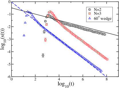
Figure 1: Log-log plot of survival probability distribution versus time for $N=2$ and $N=3$ vicious accelerating walkers in line and for a single accelerating walker in a 60^∘ wedge geometry. The line denotes a survival probability exponent of $1/4$, while the dashed line denotes a survival probability exponent of $3/4$.

Having calibrated our results for the $N=2$ case, we now consider $N=3$ vicious accelerating walkers with equal diffusion constants. The Fokker-Planck equation is given by

$$\sum_{j=1}^{3}\left[D\left(\frac{\partial^{2}}{\partial v_{j}^{2}}\right)-\left(v_{j}\frac{\partial}{\partial x_{j}}\right)\right]p(X,V,t)=\frac{\partial}{\partial t}p(X,V,t),$$ (9)

where $X=\{x_{1},x_{2},x_{3}\}$, and $V=\{v_{1},v_{2},v_{3}\}$.

We apply change of variables $v=v_{1}-v_{2}$, $u=v_{2}-v_{3}$, $x=x_{1}-x_{2}$, $y=x_{2}-x_{3}$ such that the LHS operator for two relative coordinates becomes

$$2D\left(\frac{\partial^{2}}{\partial v^{2}}+\frac{\partial^{2}}{\partial u^{2}}-\frac{\partial^{2}}{\partial v\partial u}\right)-\left(v\frac{\partial}{\partial x}+u\frac{\partial}{\partial y}\right)$$ (10)

with the absorbing boundary at $x=0$, $y=0$, $u>0$ and $v>0$. Again, here, boundary conditions on the velocities are redundant. To remove the coupled term in $u$ and $v$, we perform another set of linear transforms, $u=\frac{l-q/\sqrt{3}}{2},v=\frac{-l-q/\sqrt{3}}{2},x=\frac{-z-w/\sqrt{3}}{2},$ and $y=\frac{z-w/\sqrt{3}}{2}$ to obtain

$$6D\left(\frac{\partial^{2}}{\partial q^{2}}+\frac{\partial^{2}}{\partial l^{2}}\right)-\left(q\frac{\partial}{\partial w}+l\frac{\partial}{\partial z}\right)$$ (11)

with absorbing boundaries, $z=\pm w/\sqrt{3}$, i.e. a $60^{\circ}$ wedge in the $z-w$ plane.

We have reduced three vicious accelerating walkers in one-dimension to one accelerating walker in two-dimensions in a wedge geometry. For comparative purposes, let us review the ordinary random walker in a wedge Redner.Book . Using the conformal mapping $z^{\prime}=z^{\pi/\theta}$, one can map the wedge geometry to the upper-half plane. Then, the motion in $x$-direction becomes unbounded and in the $y$-direction it is the simple situation of a one-dimensional walker with an absorbing boundary condition. The survival probability distribution asymptotically in the upper-half plane is $s(t)\sim t^{-1/2}$. After an inverse conformal mapping, one arrives at the survival probability distribution of $s(t)\sim t^{-\pi/2\theta}$.

While there is currently no analytical solution for the survival probability distribution for an accelerating walker in a $60^{\circ}$ wedge geometry, for a $90^{\circ}$ wedge, the Sparre-Andersen theorem can be invoked for the two indepedent directions to arrive at an asymptotic power-law survival probability distribution with $\alpha=\frac{1}{2}$. In addition, for a $180^{\circ}$ wedge, $\alpha=\frac{1}{4}$. While the Sparre-Andersen theorem is quite powerful and can easily be extended to as many independent dimensions as needed, the $60^{\circ}$ wedge geometry couples the two directions (for $N=3$, at least) and, therefore, the Sparre-Andersen theorem, as it stands, cannot be invoked.

However, to smoothly interpolate between the $90^{\circ}$ and $180^{\circ}$ cases, we conjecture that for other wedge angles, the survival probability distribution also asymptotes to a power-law with survival probability exponent, $\alpha$, with $\alpha$ decreasing continuously as the wedge angle increases. To this conjecture, we resort to numerical simulation of both the wedge geometry for one accelerating walker and the line geometry for three accelerating walkers. The result is presented in Fig. 1. We measure a survival probability exponent of $\alpha=0.71\pm 0.01$ for $N=3$ vicious accelerating walkers in a line, which agrees with the $60^{\circ}$ wedge geometry result (with essentially the same error bar). Also, referring back to the accelerating walker-Levy flight mapping implemented to demonstrate the $\alpha=\frac{1}{4}$ exponent for an absorbing accelerating walker in one-dimension, simulating a $\mu=1/3$ Levy flight in a $60^{\circ}$ wedge geometry with the opening angle, $\theta$, between $0^{\circ}$ and $60^{\circ}$, yields $\alpha=0.71\pm 0.03$.

Figure 2 tests our conjecture that $\alpha$ continuously decreases with increasing wedge angle. Both the numerical values of $\alpha$ for the $90^{\circ}$ and $180^{\circ}$ wedges agree well with their analytical counterparts. For comparison purposes, we have also plotted the curve $\alpha=\pi/4\theta$, which agrees with the two analytical solutions and can be viewed as a trivial extension of the random walker solution. While the agreement looks reasonable at larger angles, the deviation becomes more apparent at smaller angles. It also appears that the divergence in $\alpha$ as $\theta$ decreases to zero is slower than $1/\theta$.

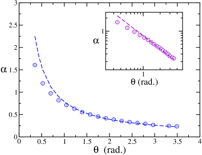
Figure 2: Survival probability exponent for a two dimensional accelerating walker in a wedge geometry as a function of the opening angle. The line denotes $\alpha=\frac{180}{4\theta}$. Inset: Log-log plot to emphasize the difference between the data and $\alpha=\frac{180}{4\theta}$. The error bars are smaller than the symbols.

III $N>3$ vicious accelerating walkers

Now, we numerically address $N>3$ vicious accelerating walkers. To compare with ordinary vicious walkers, based on the method of images, Fisher Fisher ; Fisher.Huse considered one compound walker in $N$ dimensions that cannot cross any of the $x_{1}=x_{2},x_{2}=x_{3},...,$ or $x_{N-1}=x_{N}$ linear manifolds. Using the method of images, as long as the initial positive and negative weights (corresponding to unrestricted positive and negative walkers) are chosen such that probability distribution is antisymmetric under reflection within each linear manifold, then the distribution will satisfy the absorbing boundary conditions for all future times. These weights can be represented as a Vandemond determinant, which can be factorized to yield a product of $\frac{1}{2}N(N-1)$ pairings such that $\alpha(N)=N(N-1)/4$, where $\alpha(2)=1/2$. Previous and the current simulations verify this prediction. See Figure 3. By the same argument, if the survival exponent for two (one pair of) vicious accelerating walkers is $1/4$, the survival exponent for $N$ vicious accelerating walkers system should be $N(N-1)/8$. However, for vicious accelerating walkers, the method of images fails.

Based on the $N=2$ and $N=3$ results, combined with the fact that $N$ vicious accelerating walkers can be mapped to one accelerating walker in $N-1$ dimensions in an unbounded domain, we expect the power-law survival probability distribution extends to $N>3$. In Figure 3 we present the simulation results of survival probability exponents for vicious accelerating walkers system up to $N=10$, as well as the too trivial prediction, $\alpha=N(N-1)/8$. The deviation is apparent at large $N$. We find that $N(N-1)/8$ is clearly an upper bound for the measured $N$. The non-Markovian nature of the accelerating walker enables the system to survive longer and in a way that cannot be accounted for by individual pairings.

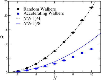
Figure 3: Survival probability exponent $\alpha$ for vicious accelerating walkers (solid squares) and vicious Gaussian walkers (solid circles) systems up to $N=10$. The simulation results for vicious Gaussian walkers agree very well with theory prediction $\alpha=N(N-1)/4$ (black curve). However, the results for vicious accelerating walkers deviate from a method of images prediction of $\alpha=N(N-1)/8$ (blue dashed curve).

IV Vicious Levy flights

As mentioned previously, vicious Gaussian walkers problem is closely related to the Gaussian random matrix theory. A matrix with random entries falls into this category as long as the entries are independent and identically distributed (iid) variables with a finite second moment of the corresponding distribution. A generalization of the random Gaussian matrix is the random Levy matrix RLM , where the entries are drawn from a broader distribution, namely a Levy distribution. The most important characteristic of Levy distribution is a heavy power-law tail step-size $S$ distribution, $P(S)\sim S^{-1-\mu}$ for large $S$. When $\mu\geq 2$, the variance of the distribution is finite and, hence, the central limit theorem holds for the distribution of the sum of independently drawn Levy variables. Similarly, the random Levy matrices reduce to random Gaussian matrices. However in the regime $\mu<2$, the variance of the distribution diverges and hence random Levy matrices behave qualitatively different from random Gaussian matrices. For example, the famous Wigner-Dyson semicircular law is replaced with a density of states that extends over the entire eigenvalue axis RLM .

Inspired by the connection between vicious Gaussian walkers and random Gaussian matrices as well as the connection between Levy flights and random accelerating walkers, we study the problem of vicious Levy flights. Given $N$ Levy flights in one-dimension, we define the vicious interaction between pairs. Because Levy flights are nonlocal, two Levy flights jump over each other without meeting at some exact point. Hence, there could be two ways to define the vicious interaction, to prohibit the jump-overs or to allow for jump-overs and the annihilation occurs upon intersection within some range, irrespective of the ordering. The latter has been recently studiedVLF . However, we are more interested in the former case, in which the set of Levy flights annihilate whenever a crossing occurs. In other words, a surviving system strictly maintains the initial ordering of all flights, which is the same as for the vicious Gaussian walkers.

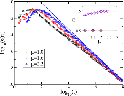
Figure 4: Log-log plot of the the survival probability distribution for $N=3$ vicious Levy flights for different values of the Levy index, $\mu$. The curve denotes a survival probability exponent of $\alpha=\frac{3}{2}$. Inset: The survival probability exponent for $N=2$ and $N=3$ vicious Levy flights as a function of the Levy index. For $\mu>2$, we obtain the vicious random walker results.

The Fokker-Planck equation for a system of $N$ one-dimensional vicious Levy flights is described as

$$\sum_{j=1}^{N}\frac{\partial^{\mu}}{\partial|x_{j}|^{\mu}}p(X,t)=\frac{\partial}{\partial t}p(X,t),$$ (12)

where the normal Laplacian is replaced by the Riesz-Feller derivative of fractional order $2>\mu>0$ Podlubny ; Samko . This derivative has an integral representation, which more easily reveals its nonlocal nature. The initial condition is still $p(X,t=0)=\prod_{j=1}^{N}\delta(x-x_{j,i})$, with $x_{j,i}<x_{k,i}$ for all $j<k$. The boundary condition for the non-crossing vicious interaction as we described above is then $p({x_{j}},t)=0$, if $x_{j}\geq x_{k}$ for any $j<k$.

The $N=2$ case is, again, equivalent to the first-passage problem of a single Levy flight via a transformation to relative coordinates (and integrating out the center of mass coordinate). The only difference with a random walker is that the absorbing boundary condition at the origin has to be modified to an absorbing region occuping the positive x-axis to preserve the non-crossing property. The first-passage property of a Levy flight is governed by the Sparre-Andersen theoremSparreAndersen ; Feller ; Majumdar , which implies that the first-passage time distribution for any symmetric step size distribution in one-dimension asymptotes to the same as that of a Gaussian walker. Thus, the survival probability exponent for $N=2$ is $\alpha=1/2$ independent of $\mu$. We verify this result in our simulation. See Figure 4. Note that this result is very different from the result obtained in Ref. VLF where $\alpha$ depends on $\mu$ for $N=2$ and higher.

We also simulate $N=3$ vicious Levy flights. Because of the linearity of fractional derivatives, the mapping of two vicious Levy flights to a single Levy flights in an absorbing plane holds. However, due to the lack of rotational invariance of the Riesz-Feller derivative, the wedge mapping that holds for vicious walkers and now for vicious accelerating walkers, does not apply to vicious Levy flights. In order to make progress, since for $N=2$ there exists a power-law distribution, we conjecture that the survival probability distribution scales as a power-law at long times for $N>2$ and measure $\alpha$. Figure 4 plots the survival probability exponents for $N=3$ vicious Levy flights for several different Levy indices. For $N=2$ all values of $\mu$ yield the same survival probability exponent of 1/2, in agreement with the Sparre-Andersen theorem. However, the $N=3$ exponents appear to vary with $\mu$. For instance, for $\mu=1$, $\alpha=1.31\pm 0.03$. While the 0.19 difference between $\mu=1.0$ and $\mu=2$ is small, the difference grows with $N$. For example, for $N=4$ and $\mu=1$, $\alpha=2.3\pm 0.1$ and for $\mu=2$, $\alpha=2.91\pm 0.09$. Based on this data, we speculate that for $N>2$, $\alpha$ depends on $\mu$.

A few comments on the technical aspects of the simulations are in order. We implement an upper cut-off on the Levy steps so that at long enough times, the survival probability distribution approaches the random walker result Mantegna . The convergence also depends on the Levy index. For example, for $\mu=1$ and stepsize cut-off $S_{c}=10-100$, the convergence to the random walker result is fast such that the asymptote to a power-law beyond $t\approx 10^{2}$ is in agreement with the random walker result to within one standard deviation. In contrast for $\mu=1.6$, $S_{c}=10^{9}$, and time scales beyond $t\approx 10^{8}$, convergence to the random walker result is observed. Secondly, for $\mu=1$ we also generated Cauchy distributed numbers directly and found good agreement with the power-law generated $\mu=1$ result.

V Conclusion

To summarize, we have generalized the vicious walker problem in two different ways: (1) vicious accelerating walkers and (2) vicious Levy flights as defined by non-crossing. For both generalizations, the typical analytical technique of the method of images fails. Analytical results for $N=2$ are readily obtainable since both problems can be mapped to the first passage problem of a single accelerating walker or Levy flight with the appropriate absorbing boundary or region. We demonstrate that the $N$ vicious walker mapping to one walker in $N-1$ dimensions in a wedge geometry generalizes to vicious accelerating walkers. We also conjecture, based on our numerical data, that there exists an upper bound on the survival probability exponent of $\alpha=\frac{1}{8}N(N-1)$ for $N$ vicious accelerating walkers. An analytical calculation for the $N=3$ case corresponding to one acclerating walker in a two-dimensional wedge geometry would be the next logical step. The heuristic argument for the absorbing accelerating walker in one-dimension using a new time counter and Levy flights may eventually become useful to analyze the two-dimensional wedge problem. There also exists a recent numerical result for the survival probability distribution for the two-dimensional Fractional Browian motion process, originally introduced by Kolmogorov Kolmogorov , in a wedge Jeon . We anticipate more study of non-Markovian processes in dimensions higher than unity in the near future. Indeed, a non-Markovian extension of Dyson’s Brownian motion model to, for example, include inertia, may be related to $N$ vicious accelerating walkers to arrive at a new class of random matrices. It may also be interesting to investigate other ordering problems of randomly accelerating walkers on a line such as the Gaussian equivalent of the ”leader” and the ”laggard” problem benAvraham .

Finally, given our numerical results, we speculate that the survival probability exponent for $N$ vicious Levy flights (as defined by no-crossing) depends on $\mu$ for fixed $N>2$. We also refer to a new result where vicious Levy flights are defined as annihilating when any two Levy flights come within some range of each other and $\alpha$ depends on $\mu$ even for $N=2$ VLF . While the survival probability exponent in one-dimension is independent of the Levy index, as a consequence of the powerful Sparre-Andersen theorem, we anticipate that this superuniversality may be broken in dimensions higher than unity and the universality of each Levy index becomes exposed. In light of our results, a higher dimensional generalization (or modification) of the Sparre-Andersen theorem should be on the forefront of at least several statistical physicists and mathematicians minds.

JMS would like to acknowledge M. Jeng for performing some preliminary simulations on no-crossing vicious Levy flights, Eli Hawkins for helpful discussion, and The Aspen Center of Physics where some of this work was conducted. JMS is supported by NSF-DMR-0645373.

*

Appendix A $N\leq 3$ mixed case

Consider a mixture of vicious accelerating and random walkers—an example of a vicious walkers system with dissimilar members. For one random walker and one random accelerator, the random walker can be approximated as an absorbing boundary at rest since the displacement of a random walker scales as $x(t)\sim t^{1/2}$, while for a random accelerating walker, the velocity scales as $v(t)\sim t^{1/2}$ such that the displacement scales as $x(t)\sim t^{3/2}$. Thus, in long time limit, the displacement of a normal random walker is negligible compared with that of a random accelerator. In other words, one can simply take the normal random walker as a fixed absorbing wall to fulfill the vicious mechanism. Simulations of one random walker and one accelerating walker that annihilate upon crossing verify this.

Now to address the $N=3$ mixed case. We use the ”A” to denote an accelerating walker and ”R” to denote a normal one in the present discussion. The two pure states ”RRR” and ”AAA” are trivial with the former following Fisher’s general solution and latter demonstrated by our numerical simulation described earlier in the paper. The combination with two normal walkers and one accelerator can have two forms, namely ”RRA” and ”RAR”. The former can be treated as one absorbing random walker and one absorbing accelerating acting independently such that $\alpha=3/4$. The latter is an accelerating walker sandwiched between two random walkers, i.e. a bounded domain, and hence the survival probability decays instead exponentially in time. A detailed analysis can be found in Ref.Bicout . Simulations support both results. See Figure 5. For ”ARA”, there is an absorbing wall in between two accelerating walkers, i.e. a pair of decoupled accelerator-wall systems, hence $\alpha=1/2$. The last possible configuration, ”AAR”, is nontrivial in that it can be reduced to one accelerating walker in a $45^{\circ}$ wedge geometry, just as two vicious random walkers in the presence of an absorbing wall can be mapped to one random walker in a $45^{\circ}$ wedge geometry. We measure a nontrivial survival probability exponent of $\alpha=0.89\pm 0.01$ for this case, which is consistent with our wedge measurements.

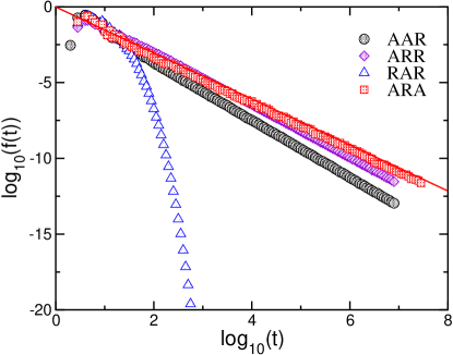
Figure 5: Log-log plot of the survival probability distribution for the $N=3$ mixed cases of vicious accelerating walkers (A) and vicious random walkers (R). The line denotes a first passage time probability exponent of $\beta=\frac{3}{2}$.

References

- (1) M. E. Fisher, Walks, walls, wetting, and melting, J. Stat. Phys. 34, 665 (1984).
- (2) D. A. Huse and M. E. Fisher, Commensurate melting, domain walls, and dislocations, Phys. Rev. B 29, 239 (1984).
- (3) F. J. Dyson, A Brownian-motion model for the eigenvalues of a random matrix, J. Math. Phys. 3, 1191 (1962).
- (4) P. J. Forrester, Vicious random walkers in the limit of a large number of walkers, J. Stat. Phys. 46, 767 (1989).
- (5) J. Baik, Random vicious walkers and random matrices, Commun. Pure Appl. Math. 53, 1385 (2000).
- (6) J. W. Essam and A. J. Guttmann, Vicious walkers and directed polymers networks in general dimensions, Phys. Rev. E 52, 5849 (1995).
- (7) M. E. Fisher and M. P. Gelfand, The reunions of three dissimilar vicious walkers, J. Stat. Phys. 53, 175 (1988).
- (8) K. Winkler and A. J. Bray, Drowsy cheetah hunting antelopes: A diffusing predator seeking fleeing prey, J. Stat. Mech. P02005 (2005).
- (9) A. J. Bray and K. Winkler, Vicious walkers in a potential, J. Phys. A 37, 5493 (2004).
- (10) R. Fukushima, A. Tanida, and K. Yano, Non-Markovian property of certain eigenvalue processes analogous to Dyson’s model, Adv. Stud. Pure Math. 57, 119 (2010).
- (11) T. W. Burkhardt, Semiflexible polymer in the half plane and statistics of the integral of a Brownian curve, J. Phys. A: Math. Gen. 26 L1157 (1993).
- (12) T. W. Marshall and E. J. Watson, J. Phys. A: Math. Gen. 18, 3531 (1985).
- (13) Y. G. Sinai, Distribution of some functionals of the integral of a random walk, Theor. Math. Phys. 90, 219 (1992).
- (14) J. M. Schwarz and R. Maimon, First-passage-time exponent for higher-order random walks: Using Levy flights, Phys. Rev. E 64, 016120 (2001).
- (15) E. Sparre Andersen, On the fluctuation of sums of random variables, Math. Scand. 1, 263 (1953).
- (16) W. Feller, An Inroduction of Probability Theory and its Applications (Wiley, New York, 1966).
- (17) S. N. Majumdar, A. Comtet, and R. M. Ziff, Unified solution of the expected maximum of a discrete time random walk and the discrete flux to a spherical trap, J. Stat. Phys. 122, 833 (2006).
- (18) P. Grassberger and W. Nadler, Go with the winners’ simulations, in: K. H. Hoffman, M. Schreiber (eds.), Computational Statistical Physics - From Billiards to Monte Carlo (Springer, Berlin, 2002), 169-190.
- (19) S. Redner, A guide to first-passage processes (New York: Cambridge University Press, 2001).
- (20) D. J. Bicout and T. W. Burkhardt, Absorption of a randomly accelerated Particle: Gambler’s ruin in a different game, J. Phys. A 33, 6835 (2000).
- (21) P. Cizeau and J. P. Bouchaud, Theory of Levy matrices, Phys. Rev. E 50, 1810 (1994).
- (22) I. Goncharenko and A. Gopinathan, Vicious Levy Flights, Phys. Rev. Lett. 105, 190601 (2010).
- (23) I. Podlubny, Fractional Differential Equations (Academic Press, London, 1999).
- (24) S. S. Samko, A. A. Kilbas, and O. I. Martichev, Fractional Integral and Derivatives (Gordon and Breach, New York, 1993).
- (25) R. A. Mantegna and H. E. Stanley, Stochastic process with ultraslow convergence to a Gaussian: The truncated Levy flight, Phys. Rev. Lett. 73, 2946 (1994).
- (26) A. N. Kolmogorov, Dolk. Acad. Sci. USSR 36, 115 (1940).
- (27) J.-H. Jeon, A. V. Chechkin, and R. Metzler, First passage behaviour of fractional Brownian motion in two-dimensional wedge domains, Eur. Phys. Lett. 94, 20008 (2011).
- (28) D. ben-Avraham, B. M. Johnson, C. A. Monaco, P. L. Krapivsky, and S. Redner, Ordering of random walks: The Leader and the Laggard, J. Phys. A: Math. Gen. 36, 1789 (2003).
*