22institutetext: Instituto de Física, Universidade do Estado do Rio de Janeiro, Rua São Francisco Xavier 524, Maracanã, 200550-900 Rio de Janeiro-RJ, Brazil
22email: claudio,joaovictor,carolina,froig,jilinski@on.br
Chemical abundances and kinematics of a sample of metal-rich barium stars ††thanks: Based on observations made with the 1.52m and 2.2m telescope at the European Southern Observatory (La Silla, Chile).,††thanks: Tables 2 and 4 are only available in electronic form at the CDS via anonymous ftp to cdsarc.u-strasbg.fr (130.79.128.5) or via http://cdsweb.u-strasbg.fr/cgi-bin/qcat?J/A+A/.
Abstract
Aims. We determined the atmospheric parameters and abundance pattern for a sample of metal-rich barium stars.
Methods. We used high-resolution optical spectroscopy. Atmospheric parameters and abundances were determined using the local thermodynamic equilibrium atmosphere models of Kurucz and the spectral analysis code MOOG.
Results. We show that the stars have enhancement factors, [s/Fe], from 0.25 to 1.16. Their abundance pattern of the Na, Al, -elements, and iron group elements as well as their kinematical properties are similar to the characteristics of the other metal-rich and super metal-rich stars already analyzed. We conclude that metal-rich barium stars do not belong to the bulge population. We also show that metal-rich barium stars are useful targets for probing the s-process enrichment in high-metallicity environments.
Key Words.:
stars: abundances — stars: chemically peculiar — stars: barium stars1 Introduction
Barium stars are chemically peculiar giant stars displaying both anomalously high heavy-element (Z 30) abundances and an overabundance of carbon compared to the Sun, with [C/Fe] varying from +0.4 to +1.2 (Antipova et al., 2004; Allen & Barbuy, 2006; Drake & Pereira, 2008; Pereira & Drake, 2009). In the mass-transfer hypothesis, the observed chemical peculiarities of these stars are a consequence of mass transfer through stellar winds or through Roche-lobe overflow in a binary system from an AGB star (now the white dwarf) to a less evolved companion, a barium giant or a subgiant CH star. Therefore, the study of their chemical peculiarities is important for understanding the physics of accretion phenomena in chemically peculiar binary systems.
Barium giants are the largest known sample among the chemically peculiar stars where the effects of the s-process nucleosynthesis can be widely investigated and measured. Busso et al. (2001) use the [hs/ls] 111[hs/ls] where [hs] and [ls] are the mean abundances of the s-elements at the Ba and Zr peaks, respectively. index as a function of metallicity as a criterion to probe whether the current models of s-process nucleosynthesis in AGB stars account for the observed abundance distributions.
Barium stars are found in the disk and in the halo of the Galaxy according to Gomez et al. (1997) and Mennessier et al. (1997). These two studies show that barium stars are an inhomogeneous group that can also be divided into groups according to their luminosities, kinematical and spatial parameters (, , velocities and dispersion velocities and scale heights). If the barium star phenomenon is seen both in the disk and in the halo, they are very useful objects to probe the s-process nucleosynthesis at different metallicities, in different population. Barium stars have already been analyzed in the halo, such as HD 206983 (Junqueira & Pereira, 2001; Drake & Pereira, 2008), HD 10613 (Pereira & Drake, 2009), and HD 123396 (Allen & Barbuy, 2006), and their connection with the metal-poor halo yellow symbiotic stars have already been investigated (Jorissen et al., 2005; Pereira & Drake, 2009). Therefore, the quantitatively confirmation of the overabundances of the s-process elements in a sample of barium stars would help to better constrain the number of known barium stars, which it would be useful to compare with their theoretical birthrate (Han et al., 1995). Motivated by the questions mentioned above, we started a high-resolution spectroscopic survey of the barium stars from the samples of MacConnell et al. (1972) and Bidelman (1981) as well as some stars from Gomez et al. (1997). As a first result of 230 surveyed stars, we have already discovered a new CH subgiant, BD-03∘3668 (Pereira & Drake, 2011).
In this paper we report another result from our survey, that is, the discovery of a small sample of 12 metal-rich ([Fe/H]+0.1) barium stars. According to their metallicities, metal-rich stars can be divided into two sub-samples (Grenon, 1972). Stars with metallicities 0.08 [Fe/H] +0.2 are the metal-rich ones and those with metallicities +0.2 [Fe/H] +0.5 are the super metal-rich. According to this scheme, we found 7 metal-rich and 5 super metal-rich barium stars. The “very metal-rich” stars were first identified by Arp (1965) investigating the nucleus of the galaxy NGC 6522. Arp (1965) also derived their age to be between 109 to 1010 Gyr. Spinrad & Taylor (1969) surveyed a large group of K giants with metal abundances greater than that of the Hyades and with abundance variations among their sample. These authors also found the giants ages to be older than the disk star, Grenon (1999) also showed that metal-rich stars have an age mixture ranging from 0.7 Gyr for the Hyades generation to an intermediate generation of 3-4 Gyr and to an oldest generation, 10 Gyr. In the investigation of the photometric and kinematic properties of a large sample of G and K giants, Eggen (1993) found that 10% of the stars in the solar neighborhood have metallicities higher than +0.15 dex. Eggen (1993) also identified a sample of barium stars among the evolved stars in the old disk population that could be metal-rich as well. However, none of the stars presented in Table 11 of his paper can be classified as metal-rich or super metal rich (HD 46407, [Fe/H] = 0.14, Antipova et al. (2003); HD 116713 and HD 202109 with respectively [Fe/H] = 0.12 and -0.04, Smiljanic et al. (2007); HD 83548, [Fe/H] = +0.03, Pereira et al. (2011) ; and NGC 2420 - D, [Fe/H] = 0.55, Smith & Suntzeff (1987)). Metal-rich stars have a mean distance from the Galactic plane of 0.2 kpc and and their Galactic orbits appear to be located inside the solar Galactic orbit (Grenon, 1999). Metal-rich stars in the solar neighborhood either could be diffused into the disk from the bulge population (Barbuy & Grenon, 1990) or they may be the representatives of the last stages of the chemical evolution of the disk (Matteucci, 2003).
We here analyze the high-resolution spectra of a sample of metal-rich barium stars to obtain [X/Fe] versus [Fe/H] trends and also to investigate the heavy-element abundance pattern in metal-rich environments. As we shall see, all our stars have spectral types G and K, and are accordingly free from the strong molecular opacity from ZrO, CN and C2 absorption features, which complicates a quantitative analysis and the measurement of some atomic lines. These molecules are usually observed in MS, S, and disk carbon stars at near solar metallicity where enhancements from s-process nucleosynthesis have already been reported (Busso et al., 2001).
2 Observations
The high-resolution spectra of our stars were obtained with the FEROS (Fiberfed Extended Range Optical Spectrograph) Echelle spectrograph (Kaufer et al., 1999) at the 1.52 m and 2.2 m ESO telescopes at La Silla (Chile) in several runs between 2000 and 2010. The FEROS spectral resolving power is , corresponding to 2.2 pixels of m, and the wavelength coverage goes from 3 800 Å to 9 200 Å. The nominal ratio was evaluated by measuring the rms flux fluctuation in selected continuum windows, and the typical values were . The spectra were reduced with the MIDAS pipeline reduction package consisting of the following standard steps: CCD bias correction, flat-fielding, spectrum extraction, wavelength calibration, correction of barycentric velocity, and spectrum rectification. Table 1 shows the log of observations and some previous information (V-magnitude, spectral types and the literature sources from where the stars were selected) of the studied stars.
| Star | Date | Exposure time | V (mag) | SpTa | Source |
|---|---|---|---|---|---|
| (sec) | |||||
| CD-25 6606 | 22/02/2008 | 1 200 | 9.3 | — | IIb |
| HD 46040 | 14/10/2008 | 420 | 8.0 | K0p | Ic |
| HD 49841 | 27/01/2001 | 3 600 | 9.0 | G5 | I |
| HD 82765 | 17/02/2008 | 600 | 8.5 | G8 III | II |
| HD 84734 | 17/02/2008 | 600 | 9.0 | — | II |
| HD 85205 | 25/03/2000 | 720 | 8.4 | G6 II | II |
| HD 100012 | 13/02/2008 | 420 | 6.6 | K0/K1 III | II |
| HD 101079 | 03/04/2007 | 600 | 8.2 | K2 | B81d |
| HD 130386 | 28/07/2009 | 420 | 7.8 | K2 | II |
| HD 139660 | 03/04/2007 | 900 | 8.4 | K0 | G97e |
| HD 198590 | 18/08/2008 | 360 | 7.0 | G8 II | II |
| HD 212209 | 18/08/2008 | 600 | 8.9 | — | II |
a: Gomez et al. (1997)
b: Table II of MacConnell et al. (1972)
c: Table I of MacConnell et al. (1972)
d: Bidelman (1981)
e: Gomez et al. (1997)
3 Analysis and results
3.1 Line selection, measurements, and oscillator strengths
Several atomic absorption lines used in this study are the same as were used in previous studies dedicated to the analysis of photospheric abundances of the barium stars (Pereira, 2005; Pereira & Drake, 2009, 2011). The chosen lines are sufficiently unblended to yield reliable abundances. Table 2 shows the Fe i and Fe ii lines employed in the analysis and also the lower excitation potential, (eV), of the transitions, the values, and the measured equivalent widths. The latter were obtained by fitting Gaussian profiles to the observed ones. The values for the Fe i and Fe ii lines were taken from Lambert et al. (1996) and Castro et al. (1997).
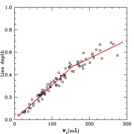
Absorption lines whose equivalent widths are not stronger than 150 mÅ should lie in the linear part of the curve of growth (Hill et al., 1995). We can evaluate if this limit is also valid for our measurements of equivalent widths by analyzing a plot of line depth vs. equivalent width. In this kind of plot we aim to examine whether (and where) there would be a significant change in the behavior of the absorption lines when the weaker and stronger lines are studied together. Figure 1 shows these measurements of several Fe i lines in the spectrum of CD-25 6606. We fitted the data using two linear functions, one between 0.0 mÅ and , and another between and 300 mÅ. By varying the value of between 100 and 200 mÅ we verified that the best fits for the two linear functions simultaneously hold for mÅ. At this point, the slope shows a reduction of about 50% (from to ). Figure 1 also shows that up to 160 mÅ the -square of fit is lower (0.0008) than the -square between 160 and 300 mÅ , which is 0.002. The change of slope and the large dispersion upward of 160 mÅ are caused by saturation effects that become important for the stronger lines so that the Gaussian profiles would not be the best representation for the line profiles. Therefore, lines with equivalent widths stronger than 160 mÅ were not used in our abundance analysis for the stars analyzed in this work. For the same reason we did not use any of the barium lines in our sample stars.
3.2 Determination of the atmospheric parameters
The determination of stellar atmospheric parameters effective temperature (Teff), surface gravity (log ), microturbulence (), and [Fe/H] (throughout, we use the notation [X/H]=log(N(X)/N(H))⋆ log(N(X)/N(H)⊙)) are prerequisites for the determination of photospheric abundances. The atmospheric parameters were determined by assuming local thermodynamic equilibrium (hereafter LTE) model atmospheres of Kurucz (1993) using the spectral analysis code MOOG (Sneden, 1973).
The solution of the excitation equilibrium used to derive the temperature (Teff) was defined by the zero slope of the trend between the iron abundances derived from FeI lines and the excitation potential of the measured lines. The microturbulent velocity () was determined by constraining the abundance determined from individual Fe i lines to show no dependence on . The solution thus found is unique, depending only on the set of Fe I,II lines and the atmospheric model employed, and yields as a by-product the metallicity of the star [Fe/H]. The final adopted atmospheric parameters are given in Table 3. The value of log seen in Table 3 was determined by means of the ionization balance using the assumption of LTE. We found typical uncertainties of (Teff) = 150 K, (log g) = 0.2 dex, and () = 0.2 km s -1.
Previous determinations of atmospheric parameters of two stars of our sample, HD 100012 and HD 130386, were made by Luck & Bond (1991) and Antipova et al. (2004), respectively. Luck & Bond (1991) found for HD 100012, Teff = 5000 K, log = 2.3 dex, Vt = 2.2 km s-1 and [Fe/H] = +0.33, while for HD 130386, Antipova et al. (2004) found Teff = 4 720 K, log = 2.4 dex, Vt = 1.4km s-1 and [Fe/H] = 0.01 dex.
| (K) | FeI/H | FeII/H | (km s-1) | (km s-1) | latitude gal. () | ||
|---|---|---|---|---|---|---|---|
| CD-25 6606 | (55) | (10) | |||||
| HD 46040 | (27) | (9) | |||||
| HD 49841 | (55) | (12) | |||||
| HD 82765 | (43) | (11) | |||||
| HD 84734 | (40) | (11) | |||||
| HD 85205 | (41) | (12) | |||||
| HD 100012 | (45) | (11) | |||||
| HD 101079 | (52) | (11) | |||||
| HD 130386 | (39) | (10) | |||||
| HD 139660 | (44) | (12) | |||||
| HD 198590 | (48) | (11) | |||||
| HD 212209 | (38) | (10) |
3.3 Abundance analysis
The abundances of chemical elements were determined with the LTE model atmosphere techniques. In brief, equivalent widths are calculated by integration through a model atmosphere and are compared with the observed equivalent widths. The calculations are repeated, changing the abundance of the element in question, until a match is achieved. The current version of the line-synthesis code moog (Sneden, 1973) was used to carry out the calculations. Table 4 shows the atomic lines used to derive the abundances of the elements. Atomic parameters for several transitions of Ti, Cr, and Ni were retrieved from the library of the National Institute of Science and Technology Atomic Spectra Database (Martin et al., 2002). Tables 5 and 6 provide the derived abundances in the notation [X/Fe]. The last two columns of Table 6 give the mean abundance of the s-process elements and their standard deviations, i.e., the scatter around the mean.
| star | [Na/Fe] | [Mg/Fe] | [Al/Fe] | [Si/Fe] | [Ca/Fe] | [Ti/Fe] | [Cr/Fe] | [Ni/Fe] |
|---|---|---|---|---|---|---|---|---|
| CD-25 6606 | +0.19 | +0.05 | -0.02 | +0.11 | +0.08 | -0.04 | +0.03 | 0.00 |
| HD 46040 | +0.16 | +0.04 | +0.02 | -0.09 | +0.11 | +0.03 | +0.06 | -0.04 |
| HD 49841 | +0.04 | -0.08 | -0.11 | -0.03 | +0.07 | -0.01 | 0.00 | +0.02 |
| HD 82765 | +0.15 | +0.18 | +0.06 | +0.15 | +0.14 | 0.00 | +0.06 | +0.08 |
| HD 84734 | +0.12 | +0.19 | -0.08 | +0.21 | +0.06 | +0.01 | +0.05 | +0.03 |
| HD 85205 | +0.23 | +0.11 | +0.11 | +0.09 | +0.08 | -0.05 | -0.01 | +0.08 |
| HD 100012 | +0.29 | +0.19 | 0.00 | +0.15 | +0.05 | +0.04 | 0.00 | +0.06 |
| HD 101079 | +0.20 | +0.14 | +0.23 | +0.19 | +0.10 | -0.06 | +0.02 | +0.03 |
| HD 130386 | +0.36 | +0.19 | +0.21 | +0.19 | +0.15 | +0.09 | +0.03 | +0.09 |
| HD 139660 | +0.23 | +0.06 | +0.07 | +0.19 | +0.07 | -0.05 | +0.03 | +0.05 |
| HD 198590 | +0.21 | +0.20 | +0.16 | +0.22 | +0.10 | -0.09 | -0.02 | +0.03 |
| HD 212209 | +0.15 | +0.12 | +0.18 | +0.20 | +0.06 | -0.03 | 0.00 | +0.07 |
| star | [Y/Fe] | [Zr/Fe] | [La/Fe] | [Ce/Fe] | [Nd/Fe] | [s/Fe] | ([s/Fe]) |
|---|---|---|---|---|---|---|---|
| CD-25 6606 | +0.62 | +0.48 | +0.73 | +0.52 | +0.85 | +0.64 | 0.15 |
| HD 46040 | +0.93 | +1.04 | +1.83 | +1.07 | +0.94 | +1.16 | 0.38 |
| HD 49841 | +0.85 | +0.65 | +0.81 | +0.56 | +0.92 | +0.76 | 0.15 |
| HD 82765 | +0.52 | +0.37 | +0.35 | +0.12 | +0.20 | +0.31 | 0.14 |
| HD 84734 | +0.64 | +0.60 | +0.74 | +0.56 | +0.80 | +0.67 | 0.10 |
| HD 85205 | +0.65 | +0.65 | +0.58 | +0.44 | +0.80 | +0.62 | 0.14 |
| HD 100012 | -0.03 | +0.13 | +0.29 | +0.25 | +0.45 | +0.22 | 0.18 |
| HD 101079 | +0.63 | +0.44 | +0.43 | +0.28 | +0.51 | +0.46 | 0.13 |
| HD 130386 | +0.65 | +0.59 | +0.47 | +0.47 | +0.29 | +0.49 | 0.14 |
| HD 139660 | +0.77 | +0.51 | +0.56 | +0.35 | +0.50 | +0.54 | 0.15 |
| HD 198590 | +0.69 | +0.51 | +0.38 | +0.33 | +0.33 | +0.45 | 0.15 |
| HD 212209 | +0.53 | +0.24 | +0.24 | +0.06 | +0.18 | +0.25 | 0.17 |
3.4 Abundance uncertainties
The uncertainties of the derived abundances for the program stars are dominated by two main sources: the errors in the stellar parameters and errors in the equivalent width measurements.
The abundance uncertainties owing to the errors in the stellar atmospheric parameters , , and were estimated by changing these parameters by their standard errors and then computing the changes incurred in the element abundances. This technique was applied in the abundances determined from equivalent line widths. The results of these calculations for CD-25∘6606 are displayed in columns 2 to 5 of Table 7. The abundance variations for the other stars show similar values.
The abundance uncertainties owing to the errors in the equivalent widths measurements were computed from an expression provided by Cayrel (1988). The errors in the equivalent widths are set, essentially, by the signal-to-noise ratio and the resolution of the spectra. In our case, having and typical S/N of 150, the expected uncertainties in the equivalent widths are about 2–3 mÅ. For all measured equivalent widths, these uncertainties lead to the errors in the abundances less than those from the sum of the uncertainties owing to the stellar parameters.
Under the assumption that the errors are independent, they can be combined quadratically so that the total uncertainty is
These final uncertainties are given in the sixth column of Table 7. The last column gives the observed abundance dispersion among the lines for those elements with more than three available lines. Table 7 also shows that neutral elements are fairly sensitive to the temperature variations, while single ionized elements are sensitive to the log variations. The uncertainties on microturbulence also contribute to the compounded errors.
| Species | obs | |||||
|---|---|---|---|---|---|---|
| K | +0.3 | +3 mÅ | ||||
| Fe i | +0.12 | 0.00 | -0.13 | +0.07 | 0.19 | 0.14 |
| Fe ii | -0.09 | +0.11 | -0.14 | +0.07 | 0.21 | 0.09 |
| Na i | +0.10 | -0.01 | -0.06 | +0.06 | 0.13 | 0.15 |
| Mg i | +0.05 | -0.03 | -0.06 | +0.04 | 0.09 | 0.18 |
| Al i | +0.07 | -0.02 | -0.05 | +0.05 | 0.10 | 0.19 |
| Si i | +0.01 | +0.02 | -0.05 | +0.06 | 0.08 | 0.06 |
| Ca i | +0.13 | -0.01 | -0.14 | +0.07 | 0.20 | 0.10 |
| Ti i | +0.28 | +0.01 | -0.07 | +0.07 | 0.29 | 0.09 |
| Cr i | +0.15 | +0.02 | -0.09 | +0.08 | 0.19 | 0.18 |
| Ni i | +0.11 | +0.03 | -0.10 | +0.07 | 0.17 | 0.12 |
| Y ii | +0.01 | +0.12 | -0.16 | +0.08 | 0.22 | 0.06 |
| Zr i | +0.21 | +0.02 | -0.01 | +0.08 | 0.23 | 0.04 |
| La ii | +0.02 | +0.13 | -0.06 | +0.07 | 0.16 | 0.19 |
| Ce ii | +0.02 | +0.13 | -0.09 | +0.08 | 0.18 | 0.11 |
| Nd ii | +0.04 | +0.15 | -0.15 | +0.10 | 0.24 | 0.14 |
4 Discussion
4.1 The position of the stars in the log - log Teff diagram.
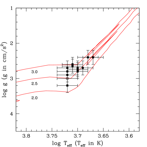
Figure 2 shows the position of the studied stars in the diagram, where model tracks were computed by Schaerer et al. (1993) for the stars of 2.0, 2.5, and 3.0 solar masses with metallicity of Z = 0.04. Putting the studied stars in this diagram, we estimated the masses as given in Table 8. Table 8 also provides the distance that resulted from the assumed mass from the diagram and from the temperature and surface gravity given in Table 3. In these calculations we assumed the bolometric corrections of Alonso et al. (1999) and Mbol⊙ = +4.74 (Bessell et al., 1998). The last column of Table 8 provides the distance of the stars whose parallax were measured by Hipparcos. The distances were derived based on the ionization equilibrium and the derived masses from the positions in the diagram, and astrometric values agree well within the uncertainties with the possible exception of HD 13966.
The stars CD-25 6606, HD 49841, HD 84734, and HD 85205, with log Teff = 3.72 and log g = 2.7, 3.2, 2.9, and 2.8 respectively, occupy a region that is at the end of subgiant phase or near the base of red giant branch in the diagram. This is important because in all high-resolution spectroscopy studies dedicated to the analyses of the spectra of barium dwarfs and CH subgiant stars, no stars of near solar metallicity or even higher than the solar metallicity in this evolutionary phase were found (Smith et al., 1993; Pereira, 2005; Allen & Barbuy, 2006). Therefore, these four stars might be the first identified metal-rich CH subgiants. Barium dwarfs (log 4.0) with metallicities close to the solar one are as yet undiscovered (Pereira & Drake, 2011).
| star | M/M⊙ | r (pc) | r (pc)(Hipparcos) |
|---|---|---|---|
| CD-25 6606 | 3.0 | 820200 | — |
| HD 46040 | 2.5 | 440100 | 32070 |
| HD 49841 | 2.0 | 31070 | — |
| HD 82765 | 2.5 | 520120 | 420140 |
| HD 84734 | 2.5 | 490115 | — |
| HD 85205 | 2.5 | 440100 | — |
| HD 100012 | 2.5 | 19045 | 18025 |
| HD 101079 | 2.5 | 39090 | — |
| HD 130386 | 2.5 | 30070 | 290110 |
| HD 139660 | 2.5 | 38090 | 19044 |
| HD 198590 | 2.5 | 26060 | 410140 |
| HD 212209 | 2.5 | 630150 | 390180 |
4.2 Kinematics
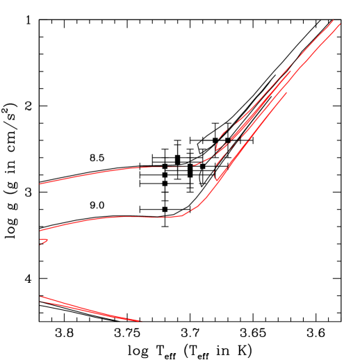
As we mentioned in the introduction, some metal-rich stars could be old objects. Figure 3 shows the position of stars analyzed in this work in the HR-diagram with the isochrones of Girardi et al. (2000). The metal-rich barium stars with ages between 8.5 and 9.0 Gyr are similar to the metal-rich stars analyzed by Pakhomov et al. (2009), which have a mean age of 8.7 Gyr. Our results confirm the results of Mennessier et al. (1997) that some barium stars in this range of gravity (and also in absolute magnitudes) have ages between 8.5 and 9.5 Gyr.
We also investigated the kinematical properties of our sample stars. Table 9 shows our results. The radial velocities were determined by measuring the Doppler shift of the spectral lines and are given in Table 3. Distances and proper motions were taken from the Hipparcos catalog (Perryman & ESA, 1997). Space velocities (U⊙, V⊙, W⊙) relative to the local standard of rest were computed based on the method of Johnson & Soderblom (1987) and were calculated assuming the solar motion of (U, V, W) = (11.1, 12.2, 7.3) km s-1, as derived by Schönrich et al. (2010). The Galactic orbital parameters Rmin and Rmax (minimum and maximum distances from the Galactic center), Zmax (maximum distance from Galactic plane) and (orbital eccentricity) were obtained using the Galactic potential integrator developed by C. Flynn (http://www.astro.utu.fi/galorb.html). For this we adopted a solar Galactocentric distance of 8.5 kpc and circular velocity of 220 km s-1. Because barium stars are binary stars, their observed radial velocities are affected by periodical variations. If we have only one determination of radial velocity, it is interesting to evaluate the uncertainties introduced by an unknown orbital motion. For this purpose we analyzed observed orbital velocity amplitude of barium binary stars with determined orbital elements (Jorissen & Mayor, 1988; Udry et al., 1998b, a). Figure 4 shows the dependence between observed orbital velocity amplitudes and the periods of analyzed stars. The mean value of the amplitude for the whole sample was found to be 6 km s-1. This value was considered as the uncertainty in the determined radial velocities of our stars.

| ULSR | VLSR | WLSR | Rmin | Rmax | Zmax | ||
|---|---|---|---|---|---|---|---|
| star | km s-1 | km s-1 | km s-1 | kpc | kpc | kpc | |
| HD 46040 | -2.3 | -2.2 | -15.0 | 7.19 | 7.95 | 0.3 | 0.05 |
| HD 82765 | 9.5 | -3.7 | 5.9 | 7.73 | 8.12 | 0.1 | 0.02 |
| HD 100012 | 11.8 | -5.1 | 4.1 | 7.53 | 8.10 | 0.1 | 0.04 |
| HD 130386 | -20.8 | -25.0 | 13.7 | 6.46 | 8.35 | 0.3 | 0.13 |
| HD 139660 | 5.5 | -26.0 | 4.7 | 6.47 | 8.20 | 0.1 | 0.12 |
| HD 198590 | -14.9 | 2.8 | 26.3 | 7.97 | 8.72 | 0.6 | 0.05 |
| HD 212209 | 50.6 | 20.0 | -7.0 | 7.60 | 10.37 | 0.4 | 0.15 |
Inspecting Table 9 we may conclude that our sample stars come from several places of the Galaxy, with mean space velocities of ULSR = 623, VLSR = 616 and WLSR = 513 km s-1. Their minimum and maximum distances to the Galactic center are 7.30.6 kpc and 8.50.8 kpc, respectively. Most of the stars have VLSR negative results, which can be taken as indication that they lag in the Galactic rotation compared to the solar motion. Two stars, HD 198590 and HD 212209, have VLSR opposite velocities compared to the rest of the stars. These properties can be taken as evidence that these metal-rich barium stars as well as other metal-rich and super metal-rich stars form an inhomogeneous group. Metal-rich stars with space velocities and/or Rmin and Rmax that differ from each other of the same studied sample would have a different star-formation history and evolution (Pakhomov et al., 2009). It also interesting to notice that HD 212209 has the highest eccentricity among the other stars. Most of the stars have Rmax less than 8.5 kpc, that is, within the solar circle, which seems to agree with the results obtained by Raboud et al. (1998) and Grenon (1999) for metal-rich stars. Other results may be seen in Table 9. All metal-rich barium stars lie inside in the (U,V)-plane of metal-rich stars of Raboud et al. (1998) and Grenon (1999), thus indicating that they display similar kinematical properties of non s-process enriched metal-rich stars. Finally, the star HD 198590 with the highest Zmax value among the analyzed stars, with a metallicity of +0.2, lies in the upper limit (with very few others) of the Zmax value in the Zmax-metallicity diagram of Grenon (1999). In Figure 13 of Soubiran & Girard (2005) this star lies between the thin-disk stars at ([Fe/H],Zmax) = (0.0, 0.1-0.2 kpc) and the thick-disk stars at ([Fe/H],Zmax)(0.5,1.0 kpc). The other stars in Table 9 belong to the thin-disk stars with lower Zmax values.
4.3 Abundances
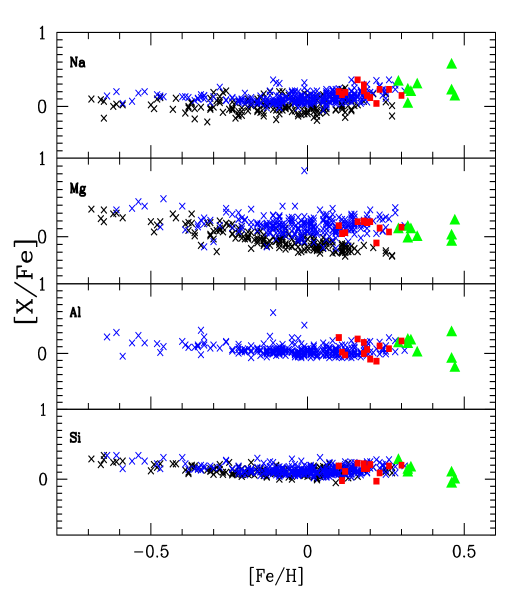
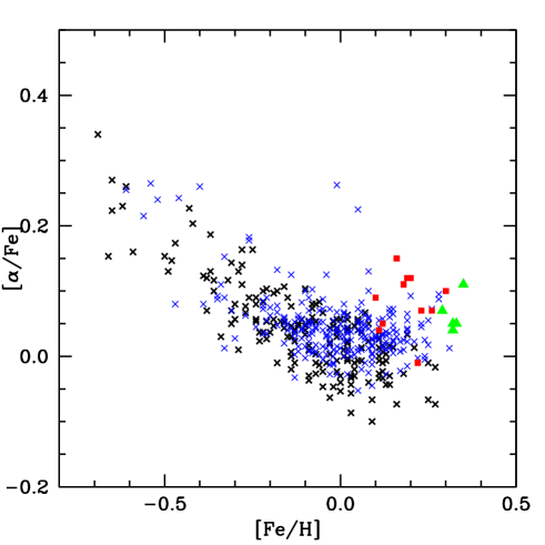
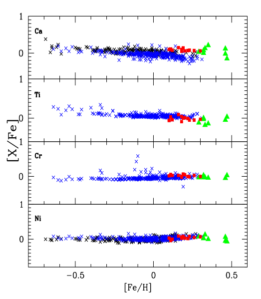
In this section we compare the abundance ratios [X/Fe] of the metal-rich barium giants analyzed in this work with the results of some studies already made for giant stars. We used for comparison the data from local disk field giants studied by Luck & Heiter (2007), disk red-clump giants studied by Mishenina et al. (2006, 2007), metal-rich giants studied by Pakhomov et al. (2009) and two metal-rich open clusters and Leo studied by Carretta et al. (2007). Figures 5 to 8 show the [X/Fe] ratios with metallicity for the barium giants of our sample and the results for the non s-process enriched giant stars mentioned above. We will see that with respect to the sodium, aluminun, -elements, chromium and nickel, the abundance ratios follow the same trend as seen in the disk-giant stars. For the heavy-elements, the [s/Fe] ratio, where ’s’ means the mean abundance of the elements synthesized by s-process, ranges from +0.2 to +1.2, thus indicating different degrees of enhancements.
4.3.1 Sodium to nickel
Sodium and aluminum are mainly produced by hydrostatic carbon burning in massive stars (Woosley & Weaver, 1995). Sodium and aluminun in disk stars has been observed among others by Edvardsson et al. (1993) and Feltzing & Gustafsson (1998). Over the range 1.0 [Fe/H] 0.0, the ratios [Na/Fe] and [Al/Fe] are slight enhanced by 0.1 dex. For metal-rich stars Edvardsson et al. (1993) and Feltzing & Gustafsson (1998) (see also Shi et al., 2004) observed an upturn in the [Na/Fe] ratio for metal-rich stars, that is [Na/Fe] = +0.2 at [Fe/H] = +0.2. Shi et al. (2004) argued that to explain this Na overabundance for the metal-rich stars, large amounts of sodium have been produced by NeNa cycle in the interiors of AGB stars. Figure 5 shows that both the local giants and the red clump giants exhibit the same trend as seen in dwarf stars. The barium giants of our sample follow the same trend. For aluminun the ratio [Al/Fe] is almost constant at 0.1 in the metallicity range 2.0 to 0.2 (Carretta et al., 2002; Edvardsson et al., 1993; Feltzing & Gustafsson, 1998). The local giants and our data for the barium giants seem to follow the same trend as seen for all these previous studies.
In the thick- and thin-disk stars the -element abundances given by the mean of Mg, Si, Ca, and Ti are overabundant by 0.2 dex at 1.0 [Fe/H] 0.5 and then decrease by 0.1-0.0 dex at 0.5 [Fe/H] 0.0 (Edvardsson et al., 1993; Reddy et al., 2003, 2006). Feltzing & Gustafsson (1998) observed that [/Fe] ratio has the same trend as detected by the other authors at 0.5 [Fe/H] 0.0. Up to [Fe/H] = +0.3 the [/Fe] ratio remains flat at [Fe/H] = 0.0-0.1. The analysis of the local disk field giants studied by Luck & Heiter (2007) and disk red-clump giants studied by Mishenina et al. (2006) showed that giants display the same trend as mentioned above for the dwarfs. Figure 6 shows that the [/Fe] ratio versus [Fe/H] for the barium stars follows the same trend as the giants. The ratios [X/Fe] for the -elements, Mg, Si, Ca, and Ti are discussed below.
Magnesium (like oxygen) is produced in massive stars at 25 M⊙ as predicted by the nucleosynthesis theory (Woosley & Weaver, 1995) and iron is mainly produced by SNeI events. It would be expected that both ratios, [O/Fe] and [Mg/Fe], would decrease with increasing metallicity. Indeed, the [O/Fe] ratio at [Fe/H] = 1.0 is +0.4, while at [Fe/H] = 0.2 is 0.1 (Edvardsson et al., 1993). In halo stars, the [Mg/Fe] ratio also increases (like oxygen) toward lower metallicities (Norris et al., 2001). In dwarf disk stars, for metallicities higher than [Fe/H] 0.2 and up to +0.2, the ratio [Mg/Fe] becomes flat at 0.1 (Feltzing & Gustafsson, 1998; Chen et al., 2000). This observed trend of the [Mg/Fe] ratio toward the higher metallicities would suggest that Mg would not only be produced by massive stars but also by type I SNe events (Chen et al., 2000). Timmes et al. (1995) predict subsolar values for the [Mg/Fe] ratio at higher metallicities for the evolution of the magnesium abundances in the Galaxy, which is not seen in all the analysis of the [Mg/Fe] ratio. The analysis of the [Mg/Fe] ratio of local giants by Luck & Heiter (2007) as well as the barium giants of our sample shows the same trend as seen in dwarfs for metallicities higher than [Fe/H] 0.0 (Figure 5). However, the [Mg/Fe] ratio for the red clump giants analyzed by Mishenina et al. (2006) behaves like the [O/Fe] ratio.
Silicon can be produced by 10-30 M⊙ stars by hydrostatic oxygen burning and also during the eventual type II supernovae explosion (Woosley & Weaver, 1986). In halo stars at [Fe/H] = 3.0 it is enhanced by +0.5 with larger scatter (Norris et al., 2001; Carretta et al., 2002). For dwarfs with metallicities higher than [Fe/H] = 0.0, it seems that silicon behaves like magnesium and has a [Si/Fe] ratio of 0.05 (Edvardsson et al., 1993). Inspecting the results of Feltzing & Gustafsson (1998), one can note that silicon flattens at a mean ratio of [Si/Fe] = 0.0 for [Fe/H] = 0.0-0.4. For the red clump giants, the local giants and the barium giants analyzed in this work the relative-to-iron silicon abundance flattens at a mean ratio of of [Si/Fe]0.1 for [Fe/H] = 0.0-0.3.
Calcium shares the same nucleosynthesis site as silicon. In halo stars it is enhanced by 0.2-0.3 dex (Norris et al., 2001). In dwarfs and for metallicities higher than [Fe/H] 0.2, calcium flattens toward a mean ratio [Ca/Fe] of 0.0. The same trend is seen in barium and red clump giants but for the local giants, the [Ca/Fe] ratio is lower by 0.2 dex at [Fe/H] = +0.2 (Luck & Heiter, 2007).
Titanium is usually considered an -element that is produced by explosive oxygen burning but could also be produced by Type Ia supernovae (Woosley & Weaver, 1995). Observationally, it behaves like an -element. Indeed, the [Ti/Fe] ratio for halo stars displays a similar trend as the [Ca/Fe] ratio. In dwarf-disk stars [Ti/Fe] slightly decreases with increasing metallicity (Edvardsson et al., 1993). For higher metallicities it seems that the ratio [Ti/Fe] flattens around 0.1. In the present work, the [Ti/Fe] ratios are usually lower than the [Mg,Si,Ca/Fe] ratios, displaying a similar trend as local-disk giants (Luck & Heiter, 2007).
The iron peak elements are formed in large amounts in Type Ia supernovae and all its members should follow the same trend with iron abundance, therefore the [X/Fe] ratios should remain constant within the range of metallicity studied. Indeed, nickel, does remain constant with [Ni/Fe] = 0.0 for 0.8 [Fe/H] 0.1. Luck & Heiter (2007) also found a tight correlation between [Fe/H] and [Ni/H] with a slope of 1.04 also between 0.8 [Fe/H] 0.1. However, some studies show a possible upturn after [Fe/H]0.1 for red clump giants (Mishenina et al., 2006; Liu et al., 2007) and dwarfs (Chen et al., 2000). This upturn is seen in Luck & Heiter’s data and also in Figure 4 of Soubiran & Girard (2005). For the element chromium, the study for the local giants of Luck & Heiter (2007) found a tight correlation between [Fe/H] and [Cr/H] with a slope of 1.06, that is [Cr/Fe] = 0.0 for 0.8 [Fe/H] 0.2, despite some discrepant points, as they reported. The barium stars of our sample also follow the general trend seen for the field giants, for the ratios of [Ni/Fe] and [Cr/Fe].
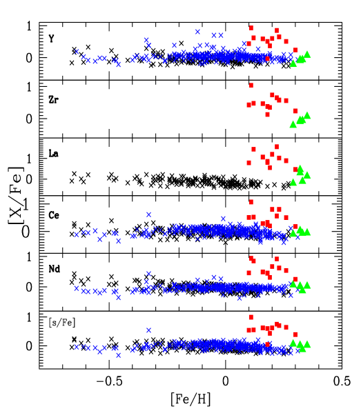
4.3.2 s-process elements : Y, Zr, La, Ce and Nd
The main site of -process elements (and also carbon) production are low-mass AGB stars (M 3.0 M⊙) during the thermally pulsing phase (TP-AGB). Nucleosynthesis of s-process takes place in the C-rich intershell convective zone, the zone between the H-burning shell and the He-burning shell, of which the source of neutrons for the s-process to occur is the 13C(,n)16O reaction (Lattanzio & Wood, 2003). Figure 8 shows the ratio [s/Fe], where ’s’ represents the mean of the elements created by slow neutron capture reactions (s-process): Y, Zr, La, Ce, and Nd. As we can see from Figure 8, all stars except HD 100012 are enhanced in the s-process elements when compared to the same ratio of the field stars. HD 100012 has a [s/Fe] ratio of +0.22 and therefore cannot be considered as a barium star because some stars at this metallicity have a similar [s/Fe] ratio as HD 157919 with [s/Fe] = +0.2 at [Fe/H] = +0.14. Among the local giants analyzed by Luck & Heiter (2007), only one barium star was spotted, HD 104979 (Zacs, 1994), which can be seen at [Fe/H] = 0.33 with [s/Fe] = +0.54.
Figure 8 also shows that our sample stars differs from the field stars only bye the degree of s-process enrichment observed in their atmospheres. Models of galactic chemical evolution do not predict this enrichment at this metallicity (Travaglio et al., 1999, 2004). Therefore, the atmospheres of these stars were contaminated either through the stellar evolution or an extrinsic event that may have happened in the past, i.e., mass-transfer hypothesis. The first hypothesis can be ruled out because of their position in the log - log Teff diagram (Figure 2). Finally, Figure 8 also shows that the abundance of zirconium is poorly investigated in normal giant stars in this metallicity range.
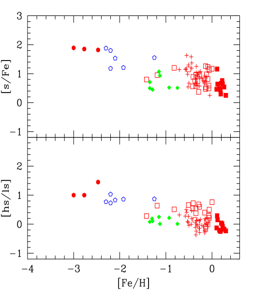
Figure 9 shows the [s/Fe] ratios for chemically peculiar binary systems including not only the barium stars (giants and dwarfs) but also the yellow symbiotic stars, the CH stars, and the CEMP (carbon enhanced metal-poor) stars, those that have already been proved as binary systems. The definition of ‘s’ varies from author to author and in some cases depends on the quality and/or on the wavelength range of the available spectra. Among CEMP stars, there are six that are binaries: CS 22942-019, CS 22948-027, CS 29497-030, CS 29497-034, CS 22964-161, and HE 0024-2523, the data of which concerning their carbon and heavy-element (Z 56) overabundances and binarity were taken from the results of Preston & Sneden (2001); Sivarani et al. (2004); Barbuy et al. (2005); Lucatello et al. (2003); Thompson et al. (2008); Aoki et al. (2002) and Hill et al. (2000). According to the mass-transfer hyphotesis for the origin of the barium stars, one of the binary components ejects its envelope that is enriched in the s-process elements produced during the AGB phase, and this matter falls onto the companion, which in turn becomes enriched in these elements, and now is the barium star. The different ratios [s/Fe] observed among the barium stars, also seen in this study, depend on the material received by the companion as well as whether this material is partially or fully mixed in the atmosphere of the barium stars. Theoretical studies for the production of the s-process elements in intrinsic AGB stars (Gallino et al., 1998; Busso et al., 1999) indicate that there is a trend that the s-process elements are more easily produced at lower metallicities as a result of the operation of the reaction 13C(,n)16O as a neutron source. When several classes of chemically-peculiar stars are examined all together (Figure 9), this phenomenon is observed.
According to Busso et al. (1999) and Travaglio et al. (2004), the neutron-capture nucleosynthesis in AGB stars is metallicity-dependent. Among the elements created by the s-process nucleosynthesis, the first neutron magic peak elements (such as Y and Zr) are the dominant products of the neutron captures in AGB models at metallicities around [Fe/H] = 0.4. At lower metallicities, [Fe/H]1.0, the second neutron magic peak elements (Ba-La-Ce-Nd) are the dominant. The origin of these two peaks is the result of the neutron magic numbers 50 and 82 nuclei, which have smaller absorption cross-sections than their neighbor nuclei and therefore turn out to be more stable than others. Owing to this, it is possible to monitor the s-process efficiency through the relative abundances of the second-peak elements to the first-peak elements. In this way the s-elements at the second-peak are usually referred to as the “heavy” s-process elements, in our case, La, Ce, and Nd, while s-elements at the first-peak are usually referred to as the “light” elements, in our case, Y and Zr. Thus, the average logarithmic ratio [hs/ls] has been widely used to measure the efficiency of neutron captures. Table 10 provides the ratios [ls/Fe], [hs/Fe] as well as the ratio [hs/ls] for the studied stars. Inspecting Table 10, we see that our derived values for the indices [hs/ls], [hs/Fe], [ls/Fe] for all metal-rich barium stars, except for HD 46040, are in the range, 0.3 to 0.0, 0.2 to 0.7 and 0.4 to 0.8. These values seem to agree well when compared with model predictions given by Busso et al. (2001) as seen in their Figures 7, 8, and 9 for the ratios [hs/ls], [hs/Fe], [ls/Fe] vs metallicity for the standard case (ST/1.5). The ST case corresponds to 410-6 M⊙ of 13C for AGB stars between 1.5 and 3.0 M⊙ for a metallicity of [Fe/H] = 0.3, which accounts for the main component of the s-process in solar system (Busso et al., 2001). HD 46040 has higher values for the indices [hs/ls] and [hs/Fe] for a star at this metallicity and its [ls/Fe] index marginally falls in the limit of the model predictions.
| star | [ls/Fe] | [hs/Fe] | [hs/ls] |
|---|---|---|---|
| CD-25 6606 | 0.55 | 0.70 | 0.15 |
| HD 46040 | 0.99 | 1.28 | 0.29 |
| HD 49841 | 0.75 | 0.76 | 0.01 |
| HD 82765 | 0.43 | 0.22 | -0.21 |
| HD 84734 | 0.62 | 0.66 | 0.04 |
| HD 85205 | 0.70 | 0.61 | -0.09 |
| HD 101079 | 0.54 | 0.41 | -0.13 |
| HD 130386 | 0.62 | 0.41 | -0.21 |
| HD 139660 | 0.64 | 0.47 | -0.17 |
| HD 198590 | 0.60 | 0.35 | -0.25 |
| HD 212209 | 0.39 | 0.16 | -0.23 |
In Figure 9 we show the [hs/ls] index as a function of the metallicity for the same classes of chemically peculiar binary systems. As for the [s/Fe] ratio vs metallicity, the [hs/ls] index also increases toward lower metallicities, with a large spread. In both figures we can see that the position of metal-rich barium stars are useful targets for constraining models for the nucleosynthesis of the s-process at higher metallicities.
5 Conclusions
Our abundance analysis has been performed by employing high-resolution optical spectra of a sample of metal-rich barium stars with the aim to obtain their abundance pattern and kinematical properties, and it can be summarized as follows:
-
1.
The stars have enhancement factors, [s/Fe], from 0.25 up to 1.16. These overabundances are expected for stars at this metallicity according to the models of Busso et al. (2001), which are based on the observed indices [ls/Fe], [hs/Fe] and [hs/ls]. The abundance pattern of the iron peak elements, of the elements of the group, as well as that of sodium and aluminum follows the disk abundance. The [alpha/Fe] ratios in our stars do not show any trace of overabundances, while bulge stars display increased ratios (Lecureur et al., 2007). Therefore, these metal-rich barium stars do not belong to the bulge population. It is probable that like the most of the non s-process enriched metal-rich stars, the barium stars analyzed in this work belong to the thin-disk stars, as can be deduced form their low Zmax values. Also interesting to note is that all stars analyzed in this work have low values for the eccentricities, which indicates almost circular orbits in agreement with this characteristic of the other non s-process enriched metal-rich stars previously analyzed (Pakhomov et al., 2009; Gratton & Sneden, 1990) and which agrees with the results of Raboud et al. (1998).
-
2.
Considering evolutionary aspects, metal-rich barium stars put another constraint on the evolution of barium dwarfs to barium giants. Because all CH subgiants and barium dwarfs analyzed so far have metallicities less than the metallicity of the Sun, except those very few subgiants analyzed in this paper, metal-rich barium dwarfs/subgiants are yet to be found. In this respect the same question can be addressed to the yellow symbiotics. All yellow symbiotics, except for the D-type, which probably are not symbiotic stars (Corradi & Schwarz, 1997; Pereira, 2005), are halo objects and their connection with metal-poor barium stars have been investigated in the recent years (Smith et al., 1996, 1997; Jorissen et al., 2005; Pereira & Roig, 2009). Consequently, disk yellow symbiotics at near solar metallicity have not yet been identified.
-
3.
Metal-rich barium stars are useful objects for investigating the heavy-element abundance pattern at metalicities higher than the metallicity of the Sun because they are free of many molecular features that are usually seen in the spectra of MS, S, and carbon stars. The barium star phenomenon once it extend toward higher metallicities, shares several properties with the non s-process enriched metal-rich and super metal-rich giant stars previously investigated.
Acknowledgements.
This research has made use of the SIMBAD database, operated at CDS, Strasbourg, France. We thank our referee for detailed comments that have improved the presentation of the present work.References
- Allen & Barbuy (2006) Allen, D. M. & Barbuy, B. 2006, A&A, 454, 917
- Alonso et al. (1999) Alonso, A., Arribas, S., & Martínez-Roger, C. 1999, A&AS, 140, 261
- Antipova et al. (2003) Antipova, L. I., Boyarchuk, A. A., Pakhomov, Y. V., & Panchuk, V. E. 2003, Astronomy Reports, 47, 648
- Antipova et al. (2004) Antipova, L. I., Boyarchuk, A. A., Pakhomov, Y. V., & Panchuk, V. E. 2004, Astronomy Reports, 48, 597
- Aoki et al. (2002) Aoki, W., Ryan, S. G., Norris, J. E., et al. 2002, ApJ, 580, 1149
- Arp (1965) Arp, H. 1965, ApJ, 141, 43
- Barbuy & Grenon (1990) Barbuy, B. & Grenon, M. 1990, in European Southern Observatory Conference and Workshop Proceedings, Vol. 35, European Southern Observatory Conference and Workshop Proceedings, ed. B. J. Jarvis & D. M. Terndrup, 83–86
- Barbuy et al. (2005) Barbuy, B., Spite, M., Spite, F., et al. 2005, A&A, 429, 1031
- Bessell et al. (1998) Bessell, M. S., Castelli, F., & Plez, B. 1998, A&A, 333, 231
- Bidelman (1981) Bidelman, W. P. 1981, AJ, 86, 553
- Biemont et al. (1981) Biemont, E., Grevesse, N., Hannaford, P., & Lowe, R. M. 1981, ApJ, 248, 867
- Busso et al. (2001) Busso, M., Gallino, R., Lambert, D. L., Travaglio, C., & Smith, V. V. 2001, ApJ, 557, 802
- Busso et al. (1999) Busso, M., Gallino, R., & Wasserburg, G. J. 1999, ARA&A, 37, 239
- Carretta et al. (2007) Carretta, E., Bragaglia, A., & Gratton, R. G. 2007, A&A, 473, 129
- Carretta et al. (2002) Carretta, E., Gratton, R., Cohen, J. G., Beers, T. C., & Christlieb, N. 2002, AJ, 124, 481
- Castro et al. (1997) Castro, S., Rich, R. M., Grenon, M., Barbuy, B., & McCarthy, J. K. 1997, AJ, 114, 376
- Cayrel (1988) Cayrel, R. 1988, in IAU Symposium, Vol. 132, The Impact of Very High S/N Spectroscopy on Stellar Physics, ed. G. Cayrel de Strobel & M. Spite, 345
- Chen et al. (2000) Chen, Y. Q., Nissen, P. E., Zhao, G., Zhang, H. W., & Benoni, T. 2000, A&AS, 141, 491
- Corradi & Schwarz (1997) Corradi, R. & Schwarz, H. E. 1997, in Physical Processes in Symbiotic Binaries and Related Systems, ed. J. Mikołajewska, 147
- Drake & Smith (1991) Drake, J. J. & Smith, G. 1991, MNRAS, 250, 89
- Drake & Pereira (2008) Drake, N. A. & Pereira, C. B. 2008, AJ, 135, 1070
- Edvardsson et al. (1993) Edvardsson, B., Andersen, J., Gustafsson, B., et al. 1993, A&A, 275, 101
- Eggen (1993) Eggen, O. J. 1993, AJ, 106, 80
- Feltzing & Gustafsson (1998) Feltzing, S. & Gustafsson, B. 1998, A&AS, 129, 237
- Gallino et al. (1998) Gallino, R., Arlandini, C., Busso, M., et al. 1998, ApJ, 497, 388
- Girardi et al. (2000) Girardi, L., Bressan, A., Bertelli, G., & Chiosi, C. 2000, A&AS, 141, 371
- Gomez et al. (1997) Gomez, A. E., Luri, X., Grenier, S., et al. 1997, A&A, 319, 881
- Gratton & Sneden (1988) Gratton, R. G. & Sneden, C. 1988, A&A, 204, 193
- Gratton & Sneden (1990) Gratton, R. G. & Sneden, C. 1990, A&A, 234, 366
- Grenon (1972) Grenon, M. 1972, in IAU Colloq. 17: Age des Etoiles, ed. G. Cayrel de Strobel & A. M. Delplace, 55
- Grenon (1999) Grenon, M. 1999, Ap&SS, 265, 331
- Han et al. (1995) Han, Z., Eggleton, P. P., Podsiadlowski, P., & Tout, C. A. 1995, MNRAS, 277, 1443
- Hannaford et al. (1982) Hannaford, P., Lowe, R. M., Grevesse, N., Biemont, E., & Whaling, W. 1982, ApJ, 261, 736
- Hill et al. (1995) Hill, V., Andrievsky, S., & Spite, M. 1995, A&A, 293, 347
- Hill et al. (2000) Hill, V., Barbuy, B., Spite, M., et al. 2000, A&A, 353, 557
- Johnson & Soderblom (1987) Johnson, D. R. H. & Soderblom, D. R. 1987, AJ, 93, 864
- Jorissen & Mayor (1988) Jorissen, A. & Mayor, M. 1988, A&A, 198, 187
- Jorissen et al. (2005) Jorissen, A., Začs, L., Udry, S., Lindgren, H., & Musaev, F. A. 2005, A&A, 441, 1135
- Junqueira & Pereira (2001) Junqueira, S. & Pereira, C. B. 2001, AJ, 122, 360
- Kaufer et al. (1999) Kaufer, A., Stahl, O., Tubbesing, S., et al. 1999, The Messenger, 95, 8
- Lambert et al. (1996) Lambert, D. L., Heath, J. E., Lemke, M., & Drake, J. 1996, ApJS, 103, 183
- Lattanzio & Wood (2003) Lattanzio, J. C. & Wood, P. R. 2003, Evolution, Nucleosynthesis and Pulsations of AGB stars., ed. H. J. Habing & H. Olofsson
- Lecureur et al. (2007) Lecureur, A., Hill, V., Zoccali, M., et al. 2007, A&A, 465, 799
- Liu et al. (2007) Liu, Y. J., Zhao, G., Shi, J. R., Pietrzyński, G., & Gieren, W. 2007, MNRAS, 382, 553
- Lucatello et al. (2003) Lucatello, S., Gratton, R., Cohen, J. G., et al. 2003, AJ, 125, 875
- Luck & Bond (1991) Luck, R. E. & Bond, H. E. 1991, ApJS, 77, 515
- Luck & Heiter (2007) Luck, R. E. & Heiter, U. 2007, AJ, 133, 2464
- MacConnell et al. (1972) MacConnell, D. J., Frye, R. L., & Upgren, A. R. 1972, AJ, 77, 384
- Martin et al. (1988) Martin, G. A., Fuhr, J. R., & Wiese, W. L. 1988, Atomic transition probabilities. Scandium through Manganese, ed. Martin, G. A., Fuhr, J. R., & Wiese, W. L.
- Martin et al. (2002) Martin, W., Fuhr, J., Kelleher, D., et al. 2002, NIST Atomic Spectra Database Version2.0 (Online Available), NIST Standard Reference Database, National Institute of Standards and Technology, Gaithersburg Maryland
- Matteucci (2003) Matteucci, F. 2003, The Chemical Evolution of the Galaxy, ed. Matteucci, F.
- McWilliam & Rich (1994) McWilliam, A. & Rich, R. M. 1994, ApJS, 91, 749
- Mennessier et al. (1997) Mennessier, M. O., Luri, X., Figueras, F., et al. 1997, A&A, 326, 722
- Mishenina et al. (2006) Mishenina, T. V., Bienaymé, O., Gorbaneva, T. I., et al. 2006, A&A, 456, 1109
- Mishenina et al. (2007) Mishenina, T. V., Gorbaneva, T. I., Bien aymé, O., et al. 2007, Astronomy Reports, 51, 382
- Norris et al. (2001) Norris, J. E., Ryan, S. G., & Beers, T. C. 2001, ApJ, 561, 1034
- Pakhomov et al. (2009) Pakhomov, Y. V., Antipova, L. I., Boyarchuk, A. A., Zhao, G., & Liang, Y. 2009, Astronomy Reports, 53, 685
- Pereira et al. (2011) Pereira, C., Roig, F., Chavero, C., & et al. 2011, in prep.
- Pereira (2005) Pereira, C. B. 2005, AJ, 129, 2469
- Pereira & Drake (2009) Pereira, C. B. & Drake, N. A. 2009, A&A, 496, 791
- Pereira & Drake (2011) Pereira, C. B. & Drake, N. A. 2011, AJ, 141, 79
- Pereira & Roig (2009) Pereira, C. B. & Roig, F. 2009, AJ, 137, 118
- Perryman & ESA (1997) Perryman, M. A. C. & ESA, eds. 1997, ESA Special Publication, Vol. 1200, The HIPPARCOS and TYCHO catalogues. Astrometric and photometric star catalogues derived from the ESA HIPPARCOS Space Astrometry Mission
- Preston & Sneden (2001) Preston, G. W. & Sneden, C. 2001, AJ, 122, 1545
- Raboud et al. (1998) Raboud, D., Grenon, M., Martinet, L., Fux, R., & Udry, S. 1998, A&A, 335, L61
- Reddy et al. (2006) Reddy, B. E., Lambert, D. L., & Allende Prieto, C. 2006, MNRAS, 367, 1329
- Reddy et al. (2003) Reddy, B. E., Tomkin, J., Lambert, D. L., & Allende Prieto, C. 2003, MNRAS, 340, 304
- Reyniers et al. (2004) Reyniers, M., Van Winckel, H., Gallino, R., & Straniero, O. 2004, A&A, 417, 269
- Schaerer et al. (1993) Schaerer, D., Charbonnel, C., Meynet, G., Maeder, A., & Schaller, G. 1993, A&AS, 102, 339
- Schönrich et al. (2010) Schönrich, R., Binney, J., & Dehnen, W. 2010, MNRAS, 403, 1829
- Shi et al. (2004) Shi, J. R., Gehren, T., & Zhao, G. 2004, A&A, 423, 683
- Sivarani et al. (2004) Sivarani, T., Bonifacio, P., Molaro, P., et al. 2004, A&A, 413, 1073
- Smiljanic et al. (2007) Smiljanic, R., Porto de Mello, G. F., & da Silva, L. 2007, A&A, 468, 679
- Smith et al. (1986) Smith, G., Edvardsson, B., & Frisk, U. 1986, A&A, 165, 126
- Smith et al. (1993) Smith, V. V., Coleman, H., & Lambert, D. L. 1993, ApJ, 417, 287
- Smith et al. (1996) Smith, V. V., Cunha, K., Jorissen, A., & Boffin, H. M. J. 1996, A&A, 315, 179
- Smith et al. (1997) Smith, V. V., Cunha, K., Jorissen, A., & Boffin, H. M. J. 1997, A&A, 324, 97
- Smith et al. (2001) Smith, V. V., Pereira, C. B., & Cunha, K. 2001, ApJ, 556, L55
- Smith & Suntzeff (1987) Smith, V. V. & Suntzeff, N. B. 1987, AJ, 93, 359
- Sneden et al. (1996) Sneden, C., McWilliam, A., Preston, G. W., et al. 1996, ApJ, 467, 819
- Sneden (1973) Sneden, C. A. 1973, PhD thesis, THE UNIVERSITY OF TEXAS AT AUSTIN.
- Soubiran & Girard (2005) Soubiran, C. & Girard, P. 2005, A&A, 438, 139
- Spinrad & Taylor (1969) Spinrad, H. & Taylor, B. J. 1969, ApJ, 157, 1279
- Thompson et al. (2008) Thompson, I. B., Ivans, I. I., Bisterzo, S., et al. 2008, ApJ, 677, 556
- Timmes et al. (1995) Timmes, F. X., Woosley, S. E., & Weaver, T. A. 1995, ApJS, 98, 617
- Travaglio et al. (1999) Travaglio, C., Galli, D., Gallino, R., et al. 1999, ApJ, 521, 691
- Travaglio et al. (2004) Travaglio, C., Gallino, R., Arnone, E., et al. 2004, ApJ, 601, 864
- Udry et al. (1998a) Udry, S., Jorissen, A., Mayor, M., & Van Eck, S. 1998a, A&AS, 131, 25
- Udry et al. (1998b) Udry, S., Mayor, M., Van Eck, S., et al. 1998b, A&AS, 131, 43
- Van Winckel & Reyniers (2000) Van Winckel, H. & Reyniers, M. 2000, A&A, 354, 135
- Wiese et al. (1969) Wiese, W. L., Smith, M. W., & Miles, B. M. 1969, Atomic transition probabilities. Vol. 2: Sodium through Calcium. A critical data compilation, ed. Wiese, W. L., Smith, M. W., & Miles, B. M.
- Woosley & Weaver (1986) Woosley, S. E. & Weaver, T. A. 1986, ARA&A, 24, 205
- Woosley & Weaver (1995) Woosley, S. E. & Weaver, T. A. 1995, ApJS, 101, 181
- Zacs (1994) Zacs, L. 1994, A&A, 283, 937
| Equivalent Widths (mÅ) | ||||||||||
| CD | HD | HD | HD | HD | HD | HD | ||||
| Element | (Å) | (eV) | log | -25 6606 | 46040 | 49841 | 82765 | 84734 | 85205 | 100012 |
| Fe i | 5242.49 | 3.63 | -0.970 | 118 | 125 | 113 | 127 | 127 | 137 | 134 |
| 5253.03 | 2.28 | -3.790 | — | — | — | 60 | — | 57 | 72 | |
| 5288.52 | 3.69 | -1.510 | 93 | — | — | — | 99 | 118 | — | |
| 5315.05 | 4.37 | -1.400 | 69 | — | — | — | — | 93 | — | |
| 5321.11 | 4.43 | -1.190 | — | 92 | 67 | — | 76 | 82 | 72 | |
| 5322.04 | 2.28 | -2.840 | 111 | 125 | 109 | 110 | 114 | 133 | — | |
| 5373.71 | 4.47 | -0.710 | 89 | — | — | — | 92 | 102 | 96 | |
| 5389.48 | 4.42 | -0.250 | 104 | 112 | — | — | 112 | — | — | |
| 5417.03 | 4.42 | -1.530 | 57 | — | 62 | 68 | 68 | 81 | 71 | |
| 5441.34 | 4.31 | -1.580 | 57 | — | — | 73 | 70 | 70 | 69 | |
| 5445.04 | 4.39 | 0.040 | 136 | — | — | — | — | — | — | |
| 5522.45 | 4.21 | -1.400 | 69 | — | — | — | — | — | — | |
| 5560.21 | 4.43 | -1.040 | 79 | 81 | 71 | — | 78 | — | 84 | |
| 5567.39 | 2.61 | -2.560 | 116 | — | — | — | — | — | — | |
| 5624.02 | 4.39 | -1.330 | — | — | — | — | — | 101 | 86 | |
| 5633.95 | 4.99 | -0.120 | 86 | — | — | 95 | — | 108 | 101 | |
| 5635.82 | 4.26 | -1.740 | 40 | 65 | 57 | 64 | 62 | 58 | 66 | |
| 5638.26 | 4.22 | -0.720 | 97 | — | 102 | 114 | 111 | 115 | 119 | |
| 5691.50 | 4.30 | -1.370 | 69 | — | — | — | — | 90 | — | |
| 5705.47 | 4.30 | -1.360 | 52 | 72 | 65 | 75 | 67 | 73 | 77 | |
| 5717.83 | 4.28 | -0.979 | — | 107 | 95 | — | — | — | — | |
| 5731.76 | 4.26 | -1.150 | 87 | 106 | 91 | 93 | 97 | 105 | 99 | |
| 5806.73 | 4.61 | -0.900 | 74 | 87 | 82 | 85 | 86 | 89 | 93 | |
| 5814.81 | 4.28 | -1.820 | 38 | 56 | 45 | 50 | 54 | 54 | 56 | |
| 5852.22 | 4.55 | -1.180 | 65 | — | 69 | 76 | 78 | 86 | 88 | |
| 5855.09 | 4.61 | -1.520 | — | — | — | 49 | — | — | — | |
| 5856.10 | 4.29 | -1.550 | — | — | — | 62 | — | — | — | |
| 5862.35 | 4.55 | -0.390 | — | — | — | 112 | — | — | — | |
| 5883.82 | 3.96 | -1.210 | 95 | — | — | 112 | 101 | 116 | — | |
| 5916.25 | 2.45 | -2.990 | 97 | — | — | — | — | — | — | |
| 5934.65 | 3.93 | -1.020 | 110 | — | 105 | 107 | 112 | 123 | 119 | |
| 6024.06 | 4.55 | -0.060 | 133 | — | 136 | — | — | — | — | |
| 6027.05 | 4.08 | -1.090 | 91 | 106 | 87 | 100 | — | 110 | 103 | |
| 6054.07 | 4.37 | -2.310 | — | — | — | — | — | 31 | — | |
| 6056.01 | 4.73 | -0.400 | 91 | 97 | — | 99 | 96 | 100 | 103 | |
| 6078.50 | 4.80 | -0.340 | — | — | — | 105 | — | — | — | |
| 6079.01 | 4.65 | -0.970 | 68 | — | 70 | 75 | 76 | 79 | 82 | |
| 6082.71 | 2.22 | -3.580 | — | — | 80 | — | — | — | — | |
| 6093.64 | 4.61 | -1.350 | — | — | 54 | 54 | 66 | 63 | 65 | |
| 6094.37 | 4.65 | -1.940 | — | — | 39 | — | — | — | — | |
| 6096.66 | 3.98 | -1.780 | — | 75 | 63 | 70 | 68 | 74 | 75 | |
| 6120.25 | 0.91 | -5.950 | 21 | 64 | 33 | — | 32 | 40 | 51 | |
| 6151.62 | 2.18 | -3.290 | 87 | 117 | 95 | 105 | 100 | 111 | 108 | |
| 6157.73 | 4.08 | -1.110 | 105 | — | — | — | — | 123 | 118 | |
| 6165.36 | 4.14 | -1.470 | 68 | 80 | 73 | 78 | 82 | 88 | 83 | |
| 6173.34 | 2.22 | -2.880 | 115 | — | 114 | 130 | — | — | — | |
| 6180.20 | 2.73 | -2.650 | — | — | 98 | — | — | — | — | |
| 6187.99 | 3.94 | -1.570 | 73 | 98 | 83 | 91 | 88 | 85 | 92 | |
| 6200.31 | 2.60 | -2.440 | 112 | — | 118 | 123 | 126 | — | 133 | |
| 6213.43 | 2.22 | -2.480 | 126 | — | — | — | — | — | — | |
| 6253.83 | 4.73 | -1.660 | — | — | 39 | — | — | — | — | |
| 6315.81 | 4.07 | -1.710 | — | — | 72 | — | — | — | — | |
| 6322.69 | 2.59 | -2.430 | 117 | — | 124 | 132 | — | — | 135 | |
| 6380.74 | 4.19 | -1.320 | — | — | 89 | — | 98 | 102 | 104 | |
| 6419.95 | 4.73 | -0.090 | — | — | 111 | — | — | — | — | |
| 6436.41 | 4.19 | -2.460 | 27 | — | 39 | 37 | — | — | 41 | |
| 6469.19 | 4.83 | -0.620 | 93 | — | 97 | — | 100 | — | — | |
| 6496.47 | 4.79 | -0.570 | — | — | 89 | — | — | — | — | |
| 6498.95 | 0.96 | -4.630 | — | — | — | 121 | — | — | — | |
| 6518.37 | 2.83 | -2.300 | — | — | — | 130 | — | — | — | |
| 6533.93 | 4.56 | -1.460 | — | — | 57 | — | — | — | — | |
| 6574.23 | 0.99 | -5.020 | 73 | — | — | — | 98 | — | 106 | |
| 6591.31 | 4.59 | -2.070 | 38 | — | 26 | — | — | — | — | |
| 6597.56 | 4.79 | -0.920 | 63 | 72 | 59 | 71 | 65 | 74 | 76 | |
| 6608.03 | 2.28 | -4.030 | 49 | — | 55 | 64 | 61 | — | 69 | |
| 6609.11 | 2.56 | -2.690 | 111 | — | 123 | — | — | — | — | |
| 6627.55 | 4.55 | -1.680 | — | — | 60 | — | — | — | — | |
| 6633.75 | 4.56 | -0.800 | — | — | 88 | — | — | — | — | |
| 6646.93 | 2.61 | -3.990 | 42 | — | — | — | — | — | — | |
| 6653.85 | 4.14 | -2.520 | 22 | — | 25 | 35 | — | — | 33 | |
| 6699.14 | 4.59 | -2.190 | — | 41 | 30 | 51 | 29 | 30 | 30 | |
| 6703.57 | 2.76 | -3.160 | 76 | — | — | — | — | — | — | |
| 6704.48 | 4.22 | -2.660 | — | 25 | 20 | 27 | 20 | — | 19 | |
| 6713.74 | 4.79 | -1.600 | 38 | 46 | 44 | 47 | 43 | — | 52 | |
| 6725.36 | 4.10 | -2.300 | — | — | 39 | — | — | 58 | — | |
| 6726.67 | 4.61 | -1.000 | — | — | 73 | — | — | — | — | |
| 6733.15 | 4.64 | -1.580 | — | — | 53 | — | — | — | — | |
| 6739.52 | 1.56 | -4.950 | 40 | 74 | 47 | 53 | 54 | 43 | 61 | |
| 6745.96 | 4.07 | -2.770 | — | 21 | 17 | — | — | — | 25 | |
| 6750.15 | 2.42 | -2.620 | 125 | — | — | — | — | — | — | |
| 6752.71 | 4.64 | -1.200 | 73 | — | — | — | — | 93 | — | |
| 6793.26 | 4.07 | -2.470 | — | — | — | 40 | 26 | — | 40 | |
| 6806.85 | 2.73 | -3.210 | 73 | — | — | 82 | 86 | — | 96 | |
| 6810.26 | 4.61 | -0.990 | 73 | 84 | 74 | 79 | 82 | 79 | 86 | |
| 6820.37 | 4.64 | -1.170 | 70 | 82 | 74 | 77 | — | 75 | 85 | |
| 6851.64 | 1.61 | -5.320 | 24 | — | — | — | — | — | — | |
| 6858.15 | 4.61 | -0.930 | 80 | — | 76 | — | 83 | 95 | 81 | |
| Fe ii | 4993.35 | 2.81 | -3.670 | 70 | 70 | 67 | — | 74 | 80 | 70 |
| 5132.66 | 2.81 | -4.000 | — | — | 53 | 65 | 63 | 76 | 51 | |
| 5234.62 | 3.22 | -2.240 | 120 | 98 | 104 | 120 | 114 | 132 | 110 | |
| 5264.81 | 3.23 | -3.190 | — | — | — | 73 | — | — | — | |
| 5325.56 | 3.22 | -3.170 | 77 | — | 61 | 70 | — | 92 | 66 | |
| 5414.05 | 3.22 | -3.620 | 61 | 58 | 49 | 61 | 60 | 73 | 49 | |
| 5425.25 | 3.20 | -3.210 | 85 | 64 | 62 | 81 | 76 | 89 | 69 | |
| 5991.37 | 3.15 | -3.560 | 66 | 56 | 52 | 64 | 62 | 80 | 64 | |
| 6084.10 | 3.20 | -3.800 | 54 | — | — | 48 | 55 | 69 | 50 | |
| 6149.25 | 3.89 | -2.720 | 60 | 51 | 55 | 60 | 61 | 76 | 65 | |
| 6247.55 | 3.89 | -2.340 | — | 61 | 71 | — | 80 | 101 | — | |
| 6416.92 | 3.89 | -2.680 | 69 | 56 | 57 | 64 | 62 | 86 | 66 | |
| 6432.68 | 2.89 | -3.580 | 76 | 65 | 68 | 85 | 75 | 90 | 74 | |
| Equivalent Widths (mÅ) | ||||||||
| HD | HD | HD | HD | HD | ||||
| Element | (Å) | (eV) | log | 101079 | 130386 | 139660 | 198590 | 212209 |
| Fe i | 5242.49 | 3.63 | -0.970 | 115 | 119 | 124 | 127 | 132 |
| 5253.03 | 2.28 | -3.790 | 63 | — | 74 | — | — | |
| 5288.52 | 3.69 | -1.510 | 97 | 100 | 114 | — | — | |
| 5321.11 | 4.43 | -1.190 | 67 | 76 | 78 | 74 | 84 | |
| 5322.04 | 2.28 | -2.840 | 107 | 119 | 119 | 114 | 131 | |
| 5373.71 | 4.47 | -0.710 | 86 | 87 | 91 | 94 | 95 | |
| 5389.48 | 4.42 | -0.250 | 108 | — | — | 112 | — | |
| 5417.03 | 4.42 | -1.530 | 64 | — | 71 | 72 | 77 | |
| 5441.34 | 4.31 | -1.580 | 62 | 68 | 70 | 67 | 72 | |
| 5445.04 | 4.39 | 0.041 | 134 | — | — | — | — | |
| 5522.45 | 4.21 | -1.400 | — | — | 80 | — | 87 | |
| 5531.98 | 4.91 | -1.460 | 42 | — | — | — | — | |
| 5560.21 | 4.43 | -1.040 | 74 | 77 | 78 | 83 | 83 | |
| 5584.77 | 3.57 | -2.170 | 76 | — | — | — | — | |
| 5624.02 | 4.39 | -1.330 | 83 | — | 92 | 91 | — | |
| 5633.95 | 4.99 | -0.120 | 92 | 102 | — | — | 98 | |
| 5635.82 | 4.26 | -1.740 | 60 | 64 | 67 | 60 | 69 | |
| 5638.26 | 4.22 | -0.720 | 111 | 115 | 114 | 111 | 119 | |
| 5705.47 | 4.30 | -1.360 | 67 | 72 | 75 | 70 | 81 | |
| 5717.83 | 4.28 | -0.979 | — | — | 109 | — | — | |
| 5731.76 | 4.26 | -1.150 | 92 | 100 | 95 | 92 | 103 | |
| 5806.73 | 4.61 | -0.900 | 82 | 89 | 90 | 82 | 92 | |
| 5814.81 | 4.28 | -1.820 | 47 | 53 | 58 | 48 | 61 | |
| 5852.22 | 4.55 | -1.180 | 74 | — | 89 | 77 | — | |
| 5883.82 | 3.96 | -1.210 | 105 | 105 | 104 | 104 | 103 | |
| 5916.25 | 2.45 | -2.990 | 106 | — | — | — | — | |
| 5934.65 | 3.93 | -1.020 | 108 | 117 | 116 | 116 | 125 | |
| 6027.05 | 4.08 | -1.090 | 96 | 103 | — | 98 | 106 | |
| 6056.01 | 4.73 | -0.400 | 95 | — | 100 | 102 | 104 | |
| 6079.01 | 4.65 | -0.970 | 68 | 70 | 84 | 80 | — | |
| 6082.71 | 2.22 | -3.580 | — | — | — | 93 | — | |
| 6093.64 | 4.61 | -1.350 | 56 | 56 | 61 | 63 | 70 | |
| 6096.66 | 3.98 | -1.780 | 68 | 75 | 75 | 69 | 78 | |
| 6120.25 | 0.91 | -5.950 | — | 53 | — | 39 | 67 | |
| 6151.62 | 2.18 | -3.290 | 97 | 108 | 109 | 102 | 119 | |
| 6157.73 | 4.08 | -1.110 | 105 | — | 122 | 117 | — | |
| 6165.36 | 4.14 | -1.470 | 74 | 77 | 81 | 80 | 85 | |
| 6173.34 | 2.22 | -2.880 | 120 | — | 139 | 132 | — | |
| 6187.99 | 3.94 | -1.570 | 80 | 90 | 91 | 89 | 105 | |
| 6200.31 | 2.60 | -2.440 | 120 | — | 133 | 123 | — | |
| 6213.43 | 2.22 | -2.480 | 136 | — | — | — | — | |
| 6322.69 | 2.59 | -2.430 | 124 | — | — | — | — | |
| 6380.74 | 4.19 | -1.320 | 92 | 103 | — | 100 | — | |
| 6436.41 | 4.19 | -2.460 | 36 | — | 47 | 40 | 53 | |
| 6469.19 | 4.83 | -0.620 | 96 | — | — | 103 | — | |
| 6518.37 | 2.83 | -2.300 | — | 109 | — | — | 122 | |
| 6574.23 | 0.99 | -5.020 | — | 107 | — | 95 | 130 | |
| 6591.31 | 4.59 | -2.070 | 28 | 36 | 31 | — | — | |
| 6597.56 | 4.79 | -0.920 | 69 | 74 | 73 | 74 | 82 | |
| 6608.03 | 2.28 | -4.030 | — | 68 | — | — | — | |
| 6609.11 | 2.56 | -2.690 | 125 | — | — | — | — | |
| 6646.93 | 2.61 | -3.990 | — | — | — | 58 | — | |
| 6653.85 | 4.14 | -2.520 | 27 | 34 | 41 | 29 | 39 | |
| 6699.14 | 4.59 | -2.190 | 25 | 38 | 37 | 29 | 43 | |
| 6703.57 | 2.76 | -3.160 | — | — | — | 100 | — | |
| 6704.48 | 4.22 | -2.660 | 19 | 27 | 22 | 17 | — | |
| 6713.74 | 4.79 | -1.600 | 41 | — | 52 | 47 | 56 | |
| 6739.52 | 1.56 | -4.950 | — | 64 | — | 57 | 76 | |
| 6745.96 | 4.07 | -2.770 | — | 22 | 23 | 21 | 35 | |
| 6752.71 | 4.64 | -1.200 | — | — | — | 92 | — | |
| 6793.26 | 4.07 | -2.470 | 33 | — | 46 | — | 51 | |
| 6806.85 | 2.73 | -3.210 | 93 | 91 | — | 92 | — | |
| 6810.26 | 4.61 | -0.990 | 75 | 85 | 88 | 83 | 92 | |
| 6820.37 | 4.64 | -1.170 | 72 | 80 | 90 | 82 | 89 | |
| 6858.15 | 4.61 | -0.930 | 81 | 93 | 89 | 86 | — | |
| Fe ii | 4993.35 | 2.81 | -3.670 | 64 | 65 | 69 | 65 | 59 |
| 5132.66 | 2.81 | -4.000 | 48 | — | 59 | 66 | — | |
| 5197.56 | 3.23 | -2.250 | — | — | 117 | — | — | |
| 5234.62 | 3.22 | -2.240 | 112 | 110 | 107 | 119 | 103 | |
| 5284.10 | 2.89 | -3.010 | — | — | — | — | 77 | |
| 5325.56 | 3.22 | -3.170 | 63 | 61 | — | 73 | 66 | |
| 5414.05 | 3.22 | -3.620 | 51 | 41 | 55 | 64 | 53 | |
| 5425.25 | 3.20 | -3.210 | 66 | 57 | 61 | 76 | — | |
| 5991.37 | 3.15 | -3.560 | 60 | 55 | 61 | 68 | 55 | |
| 6084.10 | 3.20 | -3.800 | 46 | 43 | 47 | 60 | — | |
| 6149.25 | 3.89 | -2.720 | 53 | 48 | 58 | 60 | 47 | |
| 6247.55 | 3.89 | -2.340 | — | — | 69 | — | 59 | |
| 6416.92 | 3.89 | -2.680 | 63 | 55 | 59 | 65 | 57 | |
| 6432.68 | 2.89 | -3.580 | 69 | 63 | 65 | 82 | 59 | |
| Equivalent widths (mÅ) | ||||||||||
| CD | HD | HD | HD | HD | HD | |||||
| (Å) | Species | (eV) | log | Ref | -25 6606 | 46040 | 49841 | 82765 | 84734 | 85205 |
| 5682.65 | Na i | 2.10 | -0.700 | PS | 140 | — | — | — | 148 | — |
| 5688.22 | Na i | 2.10 | -0.400 | PS | — | — | 151 | — | 152 | — |
| 6154.22 | Na i | 2.10 | -1.510 | R03 | 81 | 93 | 75 | 90 | 92 | 98 |
| 6160.75 | Na i | 2.10 | -1.210 | R03 | 89 | 123 | 111 | 107 | 100 | 116 |
| 4730.04 | Mg i | 4.34 | -2.390 | R03 | — | — | — | — | 104 | — |
| 5711.10 | Mg i | 4.34 | -1.750 | R99 | 128 | 143 | 126 | 139 | 138 | 146 |
| 6318.71 | Mg i | 5.11 | -1.940 | Ca07 | 65 | 84 | 64 | 84 | — | 77 |
| 6319.24 | Mg i | 5.11 | -2.160 | Ca07 | — | 51 | 52 | 61 | 44 | — |
| 6319.49 | Mg i | 5.11 | -2.670 | Ca07 | — | 30 | 15 | 39 | — | — |
| 6965.41 | Mg i | 5.75 | -1.720 | MR94 | 41 | 71 | 64 | 71 | 75 | 69 |
| 7387.70 | Mg i | 5.75 | -0.870 | MR94 | 81 | — | — | 118 | — | 119 |
| 8712.69 | Mg i | 5.93 | -1.260 | E93 | — | — | 71 | 103 | — | 87 |
| 8717.83 | Mg i | 5.91 | -0.970 | WSM | 108 | — | 88 | 104 | 136 | 117 |
| 8736.04 | Mg i | 5.94 | -0.340 | WSM | 146 | 139 | 137 | 156 | — | — |
| 6696.03 | Al i | 3.14 | -1.481 | MR94 | — | 79 | 59 | 77 | 59 | — |
| 6698.67 | Al i | 3.14 | -1.630 | R03 | 38 | 78 | 54 | 56 | 51 | — |
| 7835.32 | Al i | 4.04 | -0.580 | R03 | 64 | — | 62 | 80 | 64 | 91 |
| 7836.13 | Al i | 4.02 | -0.400 | R03 | 69 | 91 | 79 | 95 | 77 | 95 |
| 8772.88 | Al i | 4.02 | -0.250 | R03 | 100 | 108 | 101 | 102 | 125 | — |
| 8773.91 | Al i | 4.02 | -0.070 | R03 | 123 | — | 103 | 135 | — | — |
| 5793.08 | Si i | 4.93 | -2.060 | R03 | 69 | — | — | 83 | 78 | 90 |
| 6125.03 | Si i | 5.61 | -1.540 | E93 | 51 | — | 52 | 57 | 58 | 59 |
| 6131.58 | Si i | 5.62 | -1.685 | E93 | — | 37 | 38 | 54 | — | 56 |
| 6145.02 | Si i | 5.61 | -1.430 | E93 | 58 | 47 | 52 | 61 | 57 | 68 |
| 6155.14 | Si i | 5.62 | -0.770 | E93 | 104 | 97 | 97 | 115 | 114 | 112 |
| 7760.64 | Si i | 6.20 | -1.280 | E93 | 42 | 18 | 25 | 36 | 61 | 39 |
| 7800.00 | Si i | 6.18 | -0.720 | E93 | — | — | 59 | 83 | 100 | 100 |
| 8728.01 | Si i | 6.18 | -0.360 | E93 | 105 | — | 85 | 106 | — | 105 |
| 8742.45 | Si i | 5.87 | -0.510 | E93 | 114 | 88 | 111 | 124 | 121 | 137 |
| 6161.30 | Ca i | 2.52 | -1.270 | E93 | 96 | — | — | 107 | — | 113 |
| 6166.44 | Ca i | 2.52 | -1.140 | R03 | 99 | 116 | 105 | 110 | 115 | 110 |
| 6169.04 | Ca i | 2.52 | -0.800 | R03 | 121 | 153 | 130 | 138 | 133 | 149 |
| 6169.56 | Ca i | 2.53 | -0.480 | DS91 | 146 | — | 146 | 154 | 143 | — |
| 6455.60 | Ca i | 2.51 | -1.290 | R03 | 89 | 125 | 104 | 108 | 103 | 114 |
| 6471.66 | Ca i | 2.51 | -0.690 | S86 | 125 | 146 | 128 | 136 | 132 | — |
| 4758.12 | Ti i | 2.25 | 0.425 | MFK | 75 | — | 75 | — | — | — |
| 4759.28 | Ti i | 2.25 | 0.514 | MFK | — | — | 79 | 87 | — | — |
| 4820.41 | Ti i | 1.50 | -0.439 | MFK | — | — | — | — | 109 | — |
| 4997.10 | Ti i | 0.00 | -2.118 | MFK | — | — | 85 | 92 | 87 | — |
| 5016.17 | Ti i | 0.85 | -0.574 | MFK | 114 | — | — | 129 | 127 | — |
| 5022.87 | Ti i | 0.83 | -0.434 | MFK | — | — | 125 | 128 | 128 | — |
| 5039.96 | Ti i | 0.02 | -1.130 | MFK | — | — | 134 | 144 | — | — |
| 5043.59 | Ti i | 0.84 | -1.733 | MFK | — | — | 75 | 82 | — | — |
| 5062.10 | Ti i | 2.16 | -0.464 | MFK | — | — | 48 | — | 55 | 42 |
| 5113.45 | Ti i | 1.44 | -0.880 | E93 | 60 | 91 | 63 | 72 | 61 | — |
| 5145.47 | Ti i | 1.46 | -0.574 | MFK | 72 | 112 | 83 | 86 | 85 | 86 |
| 5152.19 | Ti i | 0.02 | -2.024 | MFK | — | — | 86 | — | 92 | — |
| 5219.71 | Ti i | 0.02 | -2.292 | MFK | — | — | 95 | 99 | 93 | 91 |
| 5223.63 | Ti i | 2.09 | -0.559 | MFK | 43 | 74 | 53 | 54 | 44 | 41 |
| 5295.78 | Ti i | 1.05 | -1.633 | MFK | 40 | 79 | 48 | 54 | 51 | 55 |
| 5490.16 | Ti i | 1.46 | -0.937 | MFK | — | — | — | — | 71 | 66 |
| 5662.16 | Ti i | 2.32 | -0.109 | MFK | — | 86 | — | 77 | 74 | 74 |
| 5689.48 | Ti i | 2.30 | -0.469 | MFK | 39 | 66 | 40 | 58 | 41 | 51 |
| 5866.46 | Ti i | 1.07 | -0.871 | E93 | 97 | — | 105 | 119 | 119 | — |
| 5922.12 | Ti i | 1.05 | -1.465 | MFK | — | 95 | 66 | 70 | 82 | — |
| 5978.55 | Ti i | 1.87 | -0.496 | MFK | 54 | 102 | 64 | 60 | 70 | 61 |
| 6091.18 | Ti i | 2.27 | -0.370 | R03 | 38 | — | 51 | 59 | 51 | 53 |
| 6126.22 | Ti i | 1.05 | -1.370 | R03 | 63 | — | 72 | 80 | 79 | 76 |
| 6258.11 | Ti i | 1.44 | -0.355 | MFK | 97 | — | 102 | 113 | 111 | 118 |
| 6261.10 | Ti i | 1.43 | -0.480 | B86 | 94 | — | 112 | 121 | 108 | 119 |
| 6554.24 | Ti i | 1.44 | -1.219 | MFK | 43 | — | 64 | 68 | 59 | 51 |
| 4789.34 | Cr i | 2.54 | -0.365 | MFK | — | — | 120 | — | — | — |
| 4801.03 | Cr i | 3.12 | -0.130 | MFK | 84 | — | 83 | 100 | 96 | 108 |
| 4814.26 | Cr i | 3.09 | -1.211 | MFK | — | — | 50 | — | 42 | — |
| 4836.85 | Cr i | 3.10 | -1.137 | MFK | 43 | — | — | — | 63 | — |
| 4936.34 | Cr i | 3.11 | -0.220 | MFK | — | — | — | — | — | 86 |
| 4964.93 | Cr i | 0.94 | -2.526 | MFK | — | 107 | — | — | — | — |
| 5193.50 | Cr i | 3.42 | -0.720 | MFK | — | — | 36 | 41 | 31 | 30 |
| 5200.18 | Cr i | 3.38 | -0.650 | MFK | — | — | 63 | 59 | 62 | — |
| 5214.13 | Cr i | 3.37 | -0.740 | MFK | — | — | 35 | 39 | 36 | 39 |
| 5238.96 | Cr i | 2.71 | -1.305 | MFK | 35 | 62 | 46 | — | 42 | 52 |
| 5247.57 | Cr i | 0.96 | -1.630 | MFK | — | — | — | 146 | 141 | — |
| 5272.00 | Cr i | 3.45 | -0.421 | MFK | — | 77 | 47 | 49 | 47 | — |
| 5296.70 | Cr i | 0.98 | -1.390 | GS | 142 | — | 144 | 157 | — | — |
| 5300.75 | Cr i | 0.98 | -2.130 | GS | — | 134 | 107 | 116 | 114 | 123 |
| 5304.18 | Cr i | 3.46 | -0.692 | MFK | — | — | 34 | 49 | 39 | 30 |
| 5318.77 | Cr i | 3.44 | -0.688 | MFK | — | — | — | 43 | 38 | — |
| 5348.33 | Cr i | 1.00 | -1.290 | GS | 136 | — | 150 | — | — | — |
| 5628.65 | Cr i | 3.42 | -0.772 | MFK | — | — | 33 | 37 | 23 | — |
| 5702.32 | Cr i | 3.45 | -0.666 | MFK | 52 | — | 70 | 63 | 60 | — |
| 5783.07 | Cr i | 3.32 | -0.500 | MFK | 50 | 73 | 60 | 64 | 60 | 63 |
| 5783.87 | Cr i | 3.32 | -0.290 | GS | 77 | — | 86 | 91 | 97 | — |
| 5784.97 | Cr i | 3.32 | -0.379 | MFK | — | 80 | — | 63 | 66 | — |
| 5787.93 | Cr i | 3.32 | -0.080 | GS | 66 | 98 | 78 | 84 | 82 | 85 |
| 6330.10 | Cr i | 0.94 | -2.920 | R03 | 68 | 121 | 83 | 83 | 87 | 89 |
| 4904.42 | Ni i | 3.54 | -0.170 | MFK | — | — | 115 | — | — | — |
| 4913.98 | Ni i | 3.74 | -0.620 | MFK | 77 | — | 82 | 93 | 83 | 100 |
| 4935.83 | Ni i | 3.94 | -0.360 | MFK | 82 | 87 | 81 | 93 | 91 | 98 |
| 4953.21 | Ni i | 3.74 | -0.660 | MFK | 86 | — | 87 | 96 | 94 | 95 |
| 4967.52 | Ni i | 3.80 | -1.570 | MFK | — | — | — | 39 | 32 | — |
| 4995.66 | Ni i | 3.63 | -1.580 | MFK | — | 51 | 38 | — | 45 | — |
| 5010.94 | Ni i | 3.63 | -0.870 | MFK | 74 | 80 | — | 83 | 78 | 86 |
| 5084.11 | Ni i | 3.68 | -0.180 | E93 | 107 | — | 102 | 124 | 107 | 138 |
| 5094.42 | Ni i | 3.83 | -1.080 | MFK | 49 | 59 | 56 | 63 | 55 | — |
| 5115.40 | Ni i | 3.83 | -0.280 | R03 | 103 | — | 97 | — | 111 | 125 |
| 5157.98 | Ni i | 3.61 | -1.590 | MFK | — | — | 44 | 50 | 46 | — |
| 5197.17 | Ni i | 3.90 | -1.190 | MFK | — | — | 59 | 70 | 61 | 62 |
| 5578.73 | Ni i | 1.68 | -2.640 | MFK | 107 | — | 104 | 118 | 113 | 121 |
| 5589.37 | Ni i | 3.90 | -1.140 | MFK | — | 56 | 46 | 53 | 48 | 61 |
| 5593.75 | Ni i | 3.90 | -0.840 | MFK | 70 | 73 | 74 | 78 | 73 | 83 |
| 5643.09 | Ni i | 4.17 | -1.250 | MFK | — | 38 | 26 | 38 | 30 | — |
| 5748.36 | Ni i | 1.68 | -3.260 | MFK | — | — | 74 | 83 | 78 | — |
| 5760.84 | Ni i | 4.11 | -0.800 | MFK | 64 | — | 73 | 58 | 71 | 80 |
| 5805.23 | Ni i | 4.17 | -0.640 | MFK | 61 | 66 | 64 | 72 | 66 | 83 |
| 5996.74 | Ni i | 4.24 | -1.060 | MFK | 38 | — | 46 | 53 | 48 | 57 |
| 6053.69 | Ni i | 4.24 | -1.070 | MFK | — | 52 | — | — | 54 | 58 |
| 6086.29 | Ni i | 4.27 | -0.510 | MFK | 59 | 76 | 72 | 83 | 73 | — |
| 6108.12 | Ni i | 1.68 | -2.440 | MFK | 116 | — | 117 | 120 | 122 | — |
| 6111.08 | Ni i | 4.09 | -0.870 | MFK | 55 | 67 | 61 | 64 | 61 | 72 |
| 6128.98 | Ni i | 1.68 | -3.320 | MFK | 74 | — | 76 | 84 | 84 | 94 |
| 6130.14 | Ni i | 4.27 | -0.960 | MFK | 40 | 47 | 40 | 50 | 47 | 49 |
| 6176.82 | Ni i | 4.09 | -0.264 | R03 | 88 | 97 | 85 | 100 | 93 | 114 |
| 6177.25 | Ni i | 1.83 | -3.510 | MFK | 45 | 67 | 49 | 56 | 52 | 66 |
| 6186.72 | Ni i | 4.11 | -0.960 | MFK | 51 | 60 | 52 | 64 | 54 | 58 |
| 6204.61 | Ni i | 4.09 | -1.140 | MFK | 47 | — | 53 | 61 | 58 | 59 |
| 6223.99 | Ni i | 4.11 | -0.980 | MFK | — | — | 60 | 61 | 48 | — |
| 6230.10 | Ni i | 4.11 | -1.260 | MFK | — | — | — | 52 | 57 | 61 |
| 6322.17 | Ni i | 4.15 | -1.170 | MFK | 32 | — | 37 | 47 | 34 | — |
| 6327.60 | Ni i | 1.68 | -3.113 | MFW | 88 | — | — | 109 | 103 | — |
| 6378.26 | Ni i | 4.15 | -0.900 | MFK | 56 | — | — | 71 | 72 | — |
| 6384.67 | Ni i | 4.15 | -1.130 | MFK | 47 | — | 43 | 52 | 46 | — |
| 6482.80 | Ni i | 1.94 | -2.630 | MFW | 81 | — | 100 | 108 | 101 | — |
| 6532.88 | Ni i | 1.94 | -3.390 | MFK | 67 | 69 | 50 | 64 | 124 | — |
| 6586.33 | Ni i | 1.95 | -2.810 | MFW | 85 | — | 90 | 98 | 96 | — |
| 6598.61 | Ni i | 4.24 | -0.980 | MFK | 42 | — | 43 | 57 | 47 | — |
| 6635.14 | Ni i | 4.42 | -0.830 | MFK | 50 | — | — | — | 55 | — |
| 6643.64 | Ni i | 1.68 | -2.030 | MFW | 142 | — | — | — | — | — |
| 6767.77 | Ni i | 1.83 | -2.170 | MFW | 125 | — | — | — | — | — |
| 6772.32 | Ni i | 3.66 | -0.970 | R03 | 70 | 84 | 80 | — | 98 | — |
| 6842.04 | Ni i | 3.66 | -1.477 | MFK | 47 | 65 | 69 | — | 58 | — |
| 7788.93 | Ni i | 1.95 | -1.990 | E93 | — | — | 141 | — | — | — |
| 4883.68 | Y ii | 1.08 | 0.070 | SN96 | — | — | 145 | — | — | — |
| 5087.43 | Y ii | 1.08 | -0.170 | SN96 | 123 | 142 | 115 | 124 | 119 | — |
| 5200.41 | Y ii | 0.99 | -0.570 | SN96 | — | — | 109 | 112 | 116 | — |
| 5205.72 | Y ii | 1.03 | -0.340 | SN96 | — | — | 134 | — | — | — |
| 5289.81 | Y ii | 1.03 | -1.850 | VWR | 49 | 74 | 55 | 46 | 56 | 64 |
| 5402.78 | Y ii | 1.84 | -0.440 | R03 | 78 | 85 | 66 | 66 | 75 | 93 |
| 6127.46 | Zr i | 0.15 | -1.060 | H82 | 20 | 96 | 36 | 29 | 36 | 39 |
| 6134.57 | Zr i | 0.00 | -1.280 | B81 | 21 | 93 | 35 | 30 | 36 | 32 |
| 6140.46 | Zr i | 0.52 | -1.410 | S96 | — | 43 | 12 | — | — | — |
| 6143.18 | Zr i | 0.07 | -1.100 | B81 | 24 | 106 | 46 | 40 | 43 | 39 |
| 4934.83 | La ii | 1.25 | -0.920 | VWR | 35 | — | 28 | — | 34 | 37 |
| 5303.53 | La ii | 0.32 | -1.350 | VWR | 54 | — | 42 | 39 | 42 | 50 |
| 5880.63 | La ii | 0.23 | -1.830 | R04 | — | 87 | 36 | — | 36 | — |
| 6320.42 | La ii | 0.17 | -1.520 | VWR | 41 | 124 | 47 | 38 | 65 | 47 |
| 6390.48 | La ii | 0.32 | -1.410 | S96 | 54 | 115 | 55 | 42 | 53 | 53 |
| 6774.33 | La ii | 0.12 | -1.709 | S96 | 52 | 119 | 44 | 39 | 47 | 50 |
| 4562.37 | Ce ii | 0.48 | 0.330 | S96 | 87 | 116 | — | — | 85 | — |
| 4628.16 | Ce ii | 0.52 | 0.260 | S96 | — | — | — | — | 95 | — |
| 5117.17 | Ce ii | 1.40 | 0.010 | VWR | 28 | — | 26 | — | — | 38 |
| 5187.46 | Ce ii | 1.21 | 0.300 | VWR | 51 | 86 | — | — | 47 | 57 |
| 5274.24 | Ce ii | 1.28 | 0.389 | VWR | 58 | 80 | 53 | 49 | 57 | 72 |
| 5330.58 | Ce ii | 0.87 | 0.280 | VWR | — | — | — | 36 | — | — |
| 5472.30 | Ce ii | 1.25 | -0.190 | VWR | 40 | 61 | 33 | 24 | 40 | 30 |
| 6051.80 | Ce ii | 0.23 | -1.600 | S96 | 20 | 51 | 17 | 10 | 20 | — |
| 4811.34 | Nd ii | 0.06 | -1.015 | VWR | 71 | — | 67 | — | 69 | 87 |
| 4959.12 | Nd ii | 0.06 | -0.916 | VWR | 86 | — | — | — | — | 105 |
| 4989.95 | Nd ii | 0.63 | -0.624 | VWR | 57 | — | — | — | — | — |
| 5063.72 | Nd ii | 0.98 | -0.758 | VWR | — | — | — | — | 32 | — |
| 5092.80 | Nd ii | 0.38 | -0.510 | E93 | — | 91 | — | — | — | — |
| 5130.59 | Nd ii | 1.30 | 0.100 | SN96 | — | — | — | 38 | — | — |
| 5212.36 | Nd ii | 0.20 | -0.700 | E93 | 79 | — | 83 | — | 92 | — |
| 5234.19 | Nd ii | 0.55 | -0.460 | S96 | — | — | — | — | — | 73 |
| 5311.46 | Nd ii | 0.98 | -0.560 | SN96 | — | — | 49 | — | — | — |
| 5319.81 | Nd ii | 0.55 | -0.350 | SN96 | — | — | 74 | 63 | — | — |
| 5416.38 | Nd ii | 0.86 | -0.980 | VWR | — | 50 | — | — | — | — |
| 5431.54 | Nd ii | 1.12 | -0.457 | VWR | — | 58 | 29 | — | 33 | — |
| 5442.26 | Nd ii | 0.68 | -0.900 | SN96 | 46 | — | — | — | 54 | 65 |
| 5740.88 | Nd ii | 1.16 | -0.560 | VWR | — | — | 26 | 29 | 40 | 32 |
| 5842.39 | Nd ii | 1.28 | -0.601 | VWR | — | 40 | — | — | — | — |
| Equivalent widths (mÅ) | ||||||||||
| HD | HD | HD | HD | HD | HD | |||||
| (Å) | Species | (eV) | log | Ref | 100012 | 101079 | 130386 | 139660 | 198590 | 212209 |
| 6154.22 | Na i | 2.10 | -1.510 | R03 | 106 | 91 | 111 | 106 | 94 | 117 |
| 6160.75 | Na i | 2.10 | -1.210 | R03 | 120 | 106 | 125 | 123 | 112 | 124 |
| 4730.04 | Mg i | 4.34 | -2.390 | R03 | 121 | — | 114 | — | 113 | — |
| 5711.10 | Mg i | 4.34 | -1.750 | R99 | 141 | 132 | 143 | 148 | 138 | 156 |
| 6318.71 | Mg i | 5.11 | -1.940 | Ca07 | 76 | 69 | 84 | 76 | 78 | — |
| 6319.24 | Mg i | 5.11 | -2.160 | Ca07 | 59 | — | 63 | — | — | 81 |
| 6319.49 | Mg i | 5.11 | -2.670 | Ca07 | 46 | 37 | 41 | 40 | 41 | 49 |
| 6765.45 | Mg i | 5.75 | -1.940 | MR94 | 35 | 40 | — | — | 32 | 49 |
| 6965.41 | Mg i | 5.75 | -1.720 | MR94 | 91 | 65 | 77 | 82 | 73 | 83 |
| 7387.70 | Mg i | 5.75 | -0.870 | MR94 | 98 | 97 | 102 | 107 | — | — |
| 8712.69 | Mg i | 5.93 | -1.260 | WSM | 110 | — | 96 | — | — | 89 |
| 8717.83 | Mg i | 5.91 | -0.970 | WSM | 124 | 116 | 114 | 112 | 125 | 106 |
| 8736.04 | Mg i | 5.94 | -0.340 | WSM | — | 159 | 161 | 156 | — | 165 |
| 6696.03 | Al i | 3.14 | -1.481 | MR | 91 | 79 | 90 | 90 | 79 | 104 |
| 6698.67 | Al i | 3.14 | -1.630 | R03 | — | — | 80 | 70 | — | 90 |
| 7835.32 | Al i | 4.04 | -0.580 | R03 | 90 | 85 | 92 | 82 | 84 | 101 |
| 7836.13 | Al i | 4.02 | -0.400 | R03 | 94 | 94 | 101 | 99 | 94 | 113 |
| 8772.88 | Al i | 4.02 | -0.250 | R03 | 121 | — | 110 | 135 | 127 | 132 |
| 8773.91 | Al i | 4.02 | -0.070 | R03 | — | 140 | 152 | — | — | 162 |
| 5793.08 | Si i | 4.93 | -2.060 | R03 | 75 | 73 | 80 | 81 | 82 | — |
| 6125.03 | Si i | 5.61 | -1.540 | E93 | 58 | 56 | 70 | 66 | 62 | 71 |
| 6131.58 | Si i | 5.62 | -1.685 | E93 | 46 | 50 | 54 | 55 | 59 | 47 |
| 6145.02 | Si i | 5.61 | -1.430 | E93 | 61 | 60 | 58 | 63 | 63 | 58 |
| 6155.14 | Si i | 5.62 | -0.770 | E93 | 110 | 100 | 105 | 108 | 109 | 110 |
| 7760.64 | Si i | 6.20 | -1.280 | E93 | 39 | 31 | — | 51 | 45 | 36 |
| 7800.00 | Si i | 6.18 | -0.720 | E93 | 93 | 80 | 78 | — | 95 | 86 |
| 8728.01 | Si i | 6.18 | -0.360 | E93 | 107 | 111 | 93 | 104 | 118 | 99 |
| 8742.45 | Si i | 5.87 | -0.510 | E93 | 102 | 114 | 106 | 129 | 127 | — |
| 6161.30 | Ca i | 2.52 | -1.270 | E93 | — | — | — | 122 | 114 | 124 |
| 6166.44 | Ca i | 2.52 | -1.140 | R03 | 117 | 107 | 115 | 113 | 109 | 122 |
| 6169.04 | Ca i | 2.52 | -0.800 | R03 | 140 | 131 | 146 | 147 | 140 | 159 |
| 6169.56 | Ca i | 2.53 | -0.480 | DS91 | 157 | 147 | — | — | — | — |
| 6455.60 | Ca i | 2.51 | -1.290 | R03 | 109 | 100 | 118 | 117 | 106 | 126 |
| 6471.66 | Ca i | 2.51 | -0.690 | S86 | 143 | 134 | 147 | 145 | 139 | 145 |
| 4758.12 | Ti i | 2.25 | 0.425 | MFK | 89 | — | — | — | — | — |
| 4759.28 | Ti i | 2.25 | 0.514 | MFK | — | 85 | 94 | 92 | — | 101 |
| 4997.10 | Ti i | 0.00 | -2.118 | MFK | 106 | 87 | 103 | 102 | — | 123 |
| 5009.66 | Ti i | 0.02 | -2.259 | MFK | 116 | — | — | — | — | — |
| 5016.17 | Ti i | 0.85 | -0.574 | MFK | 131 | 118 | 142 | 132 | 129 | — |
| 5022.87 | Ti i | 0.83 | -0.434 | MFK | 146 | 125 | 141 | 136 | 128 | — |
| 5039.96 | Ti i | 0.02 | -1.130 | MFK | — | 135 | 161 | — | 152 | — |
| 5043.59 | Ti i | 0.84 | -1.733 | MFK | 83 | 70 | 95 | 89 | — | 108 |
| 5062.10 | Ti i | 2.16 | -0.464 | MFK | 59 | 52 | 71 | 64 | 46 | 81 |
| 5087.06 | Ti i | 1.43 | -0.840 | E93 | — | 80 | — | — | 79 | — |
| 5113.45 | Ti i | 1.44 | -0.880 | E93 | 85 | 69 | — | 76 | 62 | — |
| 5145.47 | Ti i | 1.46 | -0.574 | MFK | 96 | 82 | 101 | 97 | 88 | 112 |
| 5147.48 | Ti i | 0.00 | -2.012 | MFK | 124 | 110 | — | — | — | 139 |
| 5152.19 | Ti i | 0.02 | -2.024 | MFK | 121 | 91 | 110 | — | — | 137 |
| 5219.71 | Ti i | 0.02 | -2.292 | MFK | 108 | 97 | 118 | 113 | 95 | — |
| 5223.63 | Ti i | 2.09 | -0.559 | MFK | 66 | 47 | 66 | 61 | 44 | 87 |
| 5295.78 | Ti i | 1.05 | -1.633 | MFK | 60 | 51 | 69 | 64 | 49 | 81 |
| 5490.16 | Ti i | 1.46 | -0.937 | MFK | 83 | 63 | 90 | 83 | 61 | 100 |
| 5662.16 | Ti i | 2.32 | -0.109 | MFK | 81 | 70 | 87 | 84 | 73 | — |
| 5689.48 | Ti i | 2.30 | -0.469 | MFK | 54 | 48 | 67 | 62 | 39 | 72 |
| 5866.46 | Ti i | 1.07 | -0.871 | E93 | 129 | 116 | — | — | — | — |
| 5922.12 | Ti i | 1.05 | -1.465 | MFK | 89 | 71 | 86 | 98 | 84 | 106 |
| 5978.55 | Ti i | 1.87 | -0.496 | MFK | 83 | 69 | 85 | 84 | 68 | 100 |
| 6091.18 | Ti i | 2.27 | -0.370 | R03 | 61 | 52 | 76 | 68 | 57 | 83 |
| 6126.22 | Ti i | 1.05 | -1.370 | R03 | 90 | 80 | 100 | 93 | 77 | 111 |
| 6258.11 | Ti i | 1.44 | -0.355 | MFK | 119 | 105 | 123 | 113 | 111 | 136 |
| 6261.10 | Ti i | 1.43 | -0.480 | B86 | 136 | 113 | — | — | 115 | — |
| 6554.24 | Ti i | 1.44 | -1.219 | MFK | 88 | 66 | 92 | 85 | 61 | 115 |
| 4789.34 | Cr i | 2.54 | -0.365 | MFK | — | — | — | 116 | — | — |
| 4801.03 | Cr i | 3.12 | -0.130 | MFK | 96 | 90 | 96 | 95 | 91 | 99 |
| 4814.26 | Cr i | 3.09 | -1.211 | MFK | — | 51 | — | — | — | — |
| 4836.85 | Cr i | 3.10 | -1.137 | MFK | 58 | — | 65 | — | — | 70 |
| 4936.34 | Cr i | 3.11 | -0.220 | MFK | 88 | — | — | — | — | — |
| 4964.93 | Cr i | 0.94 | -2.526 | MFK | — | — | — | — | — | 116 |
| 5193.50 | Cr i | 3.42 | -0.720 | MFK | 54 | 35 | 51 | 47 | 34 | 63 |
| 5200.18 | Cr i | 3.38 | -0.650 | MFK | 69 | 62 | 66 | 67 | 59 | 81 |
| 5214.13 | Cr i | 3.37 | -0.740 | MFK | 42 | 34 | 45 | 45 | 36 | 61 |
| 5238.96 | Cr i | 2.71 | -1.305 | MFK | 50 | 62 | 52 | — | — | — |
| 5243.36 | Cr i | 3.39 | -0.567 | MFK | — | 67 | — | 77 | — | — |
| 5247.57 | Cr i | 0.96 | -1.630 | MFK | — | 136 | — | — | 144 | — |
| 5272.00 | Cr i | 3.45 | -0.421 | MFK | — | 46 | 54 | — | 45 | 71 |
| 5300.75 | Cr i | 0.98 | -2.130 | GS | 125 | 112 | 126 | 123 | 113 | 141 |
| 5304.18 | Cr i | 3.46 | -0.692 | MFK | 45 | 39 | 49 | 50 | 39 | 55 |
| 5312.86 | Cr i | 3.45 | -0.562 | MFK | — | — | — | — | 38 | 67 |
| 5318.77 | Cr i | 3.44 | -0.688 | MFK | 47 | 40 | 53 | 53 | 41 | 59 |
| 5340.45 | Cr i | 3.44 | -0.730 | MFK | — | 62 | — | — | — | 71 |
| 5628.65 | Cr i | 3.42 | -0.772 | MFK | 40 | 33 | 42 | — | 33 | 61 |
| 5702.32 | Cr i | 3.45 | -0.666 | MFK | 52 | 63 | 67 | 67 | 56 | — |
| 5781.75 | Cr i | 3.32 | -0.750 | MFK | 66 | — | — | — | — | — |
| 5783.07 | Cr i | 3.32 | -0.500 | MFK | 69 | 59 | 68 | 71 | 63 | 74 |
| 5783.87 | Cr i | 3.32 | -0.290 | GS | — | — | — | — | 97 | 104 |
| 5784.97 | Cr i | 3.32 | -0.379 | MFK | — | 59 | 69 | 77 | 65 | 86 |
| 5787.93 | Cr i | 3.32 | -0.080 | GS | 89 | 80 | 90 | 89 | 84 | 94 |
| 6330.10 | Cr i | 0.94 | -2.920 | R03 | 94 | 83 | 103 | 98 | 83 | 118 |
| 4904.42 | Ni i | 3.54 | -0.170 | MFK | 130 | 109 | — | — | — | — |
| 4913.98 | Ni i | 3.74 | -0.620 | MFK | 99 | 86 | 88 | 91 | 89 | 98 |
| 4935.83 | Ni i | 3.94 | -0.360 | MFK | 87 | 88 | 86 | 92 | 93 | 88 |
| 4953.21 | Ni i | 3.74 | -0.660 | MFK | 102 | 92 | 101 | 98 | 100 | — |
| 4967.52 | Ni i | 3.80 | -1.570 | MFK | 39 | 35 | 41 | 44 | 41 | 50 |
| 4995.66 | Ni i | 3.63 | -1.580 | MFK | 46 | 43 | 45 | 55 | 45 | — |
| 5003.75 | Ni i | 1.68 | -3.130 | MFK | 83 | — | — | — | — | 93 |
| 5010.94 | Ni i | 3.63 | -0.870 | MFK | 83 | 73 | — | — | — | 81 |
| 5084.11 | Ni i | 3.68 | -0.180 | E93 | — | 107 | 112 | 111 | 114 | — |
| 5094.42 | Ni i | 3.83 | -1.080 | MFK | 58 | 55 | 61 | 58 | 59 | — |
| 5115.40 | Ni i | 3.83 | -0.280 | R03 | — | — | — | 109 | — | — |
| 5157.98 | Ni i | 3.61 | -1.590 | MFK | 46 | 44 | 49 | 51 | 48 | 53 |
| 5197.17 | Ni i | 3.90 | -1.190 | MFK | 71 | 62 | — | 73 | 66 | — |
| 5578.73 | Ni i | 1.68 | -2.640 | MFK | 121 | 100 | — | — | — | — |
| 5587.87 | Ni i | 1.94 | -2.370 | MFK | 107 | — | — | — | — | 110 |
| 5589.37 | Ni i | 3.90 | -1.140 | MFK | 53 | 50 | 55 | 55 | 53 | 61 |
| 5593.75 | Ni i | 3.90 | -0.840 | MFK | 76 | 68 | 74 | 76 | 77 | 83 |
| 5643.09 | Ni i | 4.17 | -1.250 | MFK | 40 | 32 | 35 | 39 | 35 | — |
| 5748.36 | Ni i | 1.68 | -3.260 | MFK | 86 | 76 | 86 | 83 | 77 | 99 |
| 5760.84 | Ni i | 4.11 | -0.800 | MFK | 84 | 75 | 80 | 76 | — | — |
| 5805.23 | Ni i | 4.17 | -0.640 | MFK | 74 | 63 | 68 | 73 | 72 | 75 |
| 5847.01 | Ni i | 1.68 | -3.440 | MFK | 82 | — | — | — | — | 95 |
| 5996.74 | Ni i | 4.24 | -1.060 | MFK | 57 | 43 | 55 | 57 | 53 | — |
| 6053.69 | Ni i | 4.24 | -1.070 | MFK | — | 50 | 59 | 62 | 60 | — |
| 6086.29 | Ni i | 4.27 | -0.510 | MFK | 79 | 69 | 77 | 77 | 75 | 74 |
| 6108.12 | Ni i | 1.68 | -2.440 | MFK | 132 | 118 | 128 | 129 | 118 | 133 |
| 6111.08 | Ni i | 4.09 | -0.870 | MFK | 74 | 62 | 67 | 66 | 69 | 69 |
| 6128.98 | Ni i | 1.68 | -3.320 | MFK | 90 | 79 | 92 | 93 | 89 | 104 |
| 6130.14 | Ni i | 4.27 | -0.960 | MFK | 58 | 46 | 49 | 54 | 58 | 52 |
| 6176.82 | Ni i | 4.09 | -0.264 | R03 | 100 | 91 | 93 | 95 | 99 | 103 |
| 6177.25 | Ni i | 1.83 | -3.510 | MFK | 62 | 51 | 59 | 61 | 59 | 69 |
| 6186.72 | Ni i | 4.11 | -0.960 | MFK | 66 | 55 | 59 | 63 | 57 | 75 |
| 6204.61 | Ni i | 4.09 | -1.140 | MFK | 60 | 54 | 67 | 67 | 59 | — |
| 6223.99 | Ni i | 4.11 | -0.980 | MFK | 63 | 56 | 61 | 70 | 64 | 80 |
| 6230.10 | Ni i | 4.11 | -1.260 | MFK | — | 51 | 57 | 56 | — | — |
| 6322.17 | Ni i | 4.15 | -1.170 | MFK | 47 | 38 | 47 | 47 | 44 | — |
| 6327.60 | Ni i | 1.68 | -3.113 | MFW | 112 | 97 | — | — | 106 | — |
| 6378.26 | Ni i | 4.15 | -0.900 | MFK | — | 62 | — | 78 | 75 | — |
| 6384.67 | Ni i | 4.15 | -1.130 | MFK | — | 46 | 49 | 53 | 49 | 57 |
| 6482.80 | Ni i | 1.94 | -2.630 | MFW | 111 | 92 | 117 | 117 | 100 | — |
| 6532.88 | Ni i | 1.94 | -3.390 | MFK | — | 49 | — | 60 | 58 | 81 |
| 6586.33 | Ni i | 1.95 | -2.810 | MFW | 103 | 95 | 103 | 105 | 101 | 123 |
| 6598.61 | Ni i | 4.24 | -0.980 | MFK | 58 | 52 | — | 55 | 55 | 69 |
| 6643.64 | Ni i | 1.68 | -2.030 | MFW | — | 149 | — | 163 | — | — |
| 6767.77 | Ni i | 1.83 | -2.170 | MFW | — | 139 | — | — | — | — |
| 6772.32 | Ni i | 3.66 | -0.970 | R03 | 96 | 90 | 96 | 98 | 97 | 94 |
| 6842.04 | Ni i | 3.66 | -1.477 | MFK | 67 | 62 | — | — | 69 | — |
| 4883.68 | Y ii | 1.08 | 0.070 | SN96 | — | — | — | 154 | — | — |
| 5087.43 | Y ii | 1.08 | -0.170 | SN96 | 93 | 114 | 118 | 130 | 131 | 117 |
| 5200.41 | Y ii | 0.99 | -0.570 | SN96 | 99 | 111 | 114 | — | 124 | 118 |
| 5289.81 | Y ii | 1.03 | -1.850 | VWR | 26 | 52 | 52 | 49 | 58 | 54 |
| 5402.78 | Y ii | 1.84 | -0.440 | R03 | 50 | 68 | 68 | — | 79 | 68 |
| 6127.46 | Zr i | 0.15 | -1.060 | H82 | 28 | 37 | 63 | 52 | 37 | 68 |
| 6134.57 | Zr i | 0.00 | -1.280 | B81 | 27 | 36 | 58 | 50 | 35 | 65 |
| 6140.46 | Zr i | 0.52 | -1.410 | S96 | — | — | 20 | 19 | 13 | 25 |
| 6143.18 | Zr i | 0.07 | -1.100 | B81 | 33 | 44 | 64 | 59 | 44 | 78 |
| 4086.71 | La ii | 0.00 | -0.160 | VWR | — | — | — | 97 | 98 | — |
| 4934.83 | La ii | 1.25 | -0.920 | VWR | — | — | — | 23 | — | — |
| 5303.53 | La ii | 0.32 | -1.350 | VWR | 33 | 40 | 35 | 37 | 37 | 41 |
| 5880.63 | La ii | 0.23 | -1.830 | R04 | 26 | 22 | 38 | 36 | 38 | 39 |
| 6320.43 | La ii | 0.17 | -1.520 | VWR | 38 | 42 | 44 | 47 | 38 | 46 |
| 6390.48 | La ii | 0.32 | -1.410 | S96 | 36 | 47 | 54 | 52 | 39 | — |
| 6774.33 | La ii | 0.12 | -1.709 | S96 | 30 | 38 | 34 | — | 32 | 40 |
| 4073.47 | Ce ii | 0.48 | 0.320 | SN96 | — | — | — | 79 | 82 | — |
| 4120.84 | Ce ii | 0.32 | -0.240 | S96 | 65 | — | — | — | 72 | — |
| 4486.91 | Ce ii | 0.30 | -0.360 | S96 | — | — | 70 | — | — | — |
| 4562.37 | Ce ii | 0.48 | 0.330 | S96 | 80 | 79 | 86 | 76 | 82 | 84 |
| 4628.16 | Ce ii | 0.52 | 0.260 | S96 | 77 | — | 81 | 76 | 90 | — |
| 5117.17 | Ce ii | 1.40 | 0.010 | VWR | — | — | — | — | 24 | — |
| 5187.46 | Ce ii | 1.21 | 0.300 | VWR | — | 41 | — | — | 40 | 40 |
| 5274.24 | Ce ii | 1.28 | 0.389 | VWR | 46 | 48 | 48 | — | 47 | 44 |
| 5472.30 | Ce ii | 1.25 | -0.190 | VWR | 21 | 21 | 29 | — | 22 | 20 |
| 6051.80 | Ce ii | 0.23 | -1.600 | S96 | 13 | 15 | 20 | 18 | 15 | 21 |
| 4811.34 | Nd ii | 0.06 | -1.015 | VWR | 60 | 58 | 65 | 57 | 58 | — |
| 4989.95 | Nd ii | 0.63 | -0.624 | VWR | 50 | 56 | — | 49 | 49 | — |
| 5063.72 | Nd ii | 0.98 | -0.758 | VWR | 16 | 19 | 17 | 37 | 19 | — |
| 5092.80 | Nd ii | 0.38 | -0.510 | E93 | — | — | 49 | — | — | 59 |
| 5212.36 | Nd ii | 0.20 | -0.700 | E93 | — | — | — | — | 78 | — |
| 5234.19 | Nd ii | 0.55 | -0.460 | S96 | 58 | — | — | 60 | 58 | — |
| 5311.46 | Nd ii | 0.98 | -0.560 | SN96 | 38 | 40 | — | 36 | 37 | — |
| 5319.81 | Nd ii | 0.55 | -0.350 | SN96 | 80 | 76 | 56 | 66 | 72 | 61 |
| 5416.38 | Nd ii | 0.86 | -0.980 | VWR | — | 15 | — | — | 16 | — |
| 5431.54 | Nd ii | 1.12 | -0.457 | VWR | — | 27 | — | — | 23 | — |
| 5442.26 | Nd ii | 0.68 | -0.900 | SN96 | 49 | — | — | — | — | — |
| 5740.88 | Nd ii | 1.16 | -0.560 | VWR | 20 | 21 | — | 28 | 20 | 33 |
| 5842.39 | Nd ii | 1.28 | -0.601 | VWR | — | 31 | 15 | — | 11 | — |
| 222References to Table 4: References to Table 4: B81: Biemont et al. (1981); Ca07: Carretta et al. (2007); DS91: Drake & Smith (1991); E93: Edvardsson et al. (1993); GS: Gratton & Sneden (1988); H82: Hannaford et al. (1982); PS: Preston & Sneden (2001); R03: Reddy et al. (2003); R04: Reyniers et al. (2004); MFK: Martin et al. (2002); MFW: Martin et al. (1988); MR94: McWilliam & Rich (1994); S86: Smith et al. (1986); S96: Smith et al. (1996); SN96: Sneden et al. (1996); VWR: Van Winckel & Reyniers (2000); WSM: Wiese et al. (1969); | ||||||||||