Lattice Boltzmann Method for Electromagnetic Wave Propagation

Abstract

We present a new Lattice Boltzmann (LB) formulation to solve the Maxwell equations for electromagnetic (EM) waves propagating in a heterogeneous medium. By using a pseudo-vector discrete Boltzmann distribution, the scheme is shown to reproduce the continuum Maxwell equations. The technique compares well with a pseudo-spectral method at solving for two-dimensional wave propagation in a heterogeneous medium, which by design contains substantial contrasts in the refractive index. The extension to three dimensions follows naturally and, owing to the recognized efficiency of LB schemes for parallel computation in irregular geometries, it gives a powerful method to numerically simulate a wide range of problems involving EM wave propagation in complex media.

1 Introduction

Over the last two decades, the LB method in the Bhatnagar-Gross-Krook (BGK) approximation (see [1]) has met with significant success in simulating a broad spectrum of complex flow phenomena [2, 3], ranging from low-Reynolds flows in porous media to fully developed turbulent flows in complex geometries, multiphase flows and, more recently, relativistic flows [4]. The application of LB techniques to EM wave propagation phenomena is comparatively far less developed. Given the paramount role of EM phenomena in science and technology, including fast-emerging applications such as metamaterials and transformation optics [5], it is of great interest to investigate whether LB techniques are able to improve simulations of complex EM phenomena as they have for fluid flows.

LB schemes for wave propagation have been proposed before in literature, [6, 7, 8], but it is only recently that such schemes have been specifically tailored to EM phenomena. To this end, a basic issue had to be addressed, namely the fact that, unlike hydrodynamics, EM interactions are governed by an anti-symmetric field tensor, a structure that does not naturally emerge from standard kinetic theory. To circumvent this problem, Mendoza et al. [10, 11] proposed a scheme wherein the electric and magnetic fields are represented by separate discrete Boltzmann distributions, each moving along distinct lattice directions. Although an important conceptual advance, the resulting scheme appears computationally intensive.

A more straightforward formulation for EM wave propagation in plasmas has been recently proposed by Dellar ([12], [13]). By promoting the discrete Boltzmann distribution from a scalar to a vector quantity (also see [7], [9]), and expressing the curl of electric field in divergence form, Dellar developed an elegant and compact scheme in which magnetic field emerges as the “vector density” associated with the vector-valued discrete Boltzmann distribution. The Maxwell equations emerge when a Hermite-projection procedure is applied to the resulting kinetic equation. However, antisymmetry of the relevant EM tensor is not preserved in time, so it must be enforced at each time-step.

Motivated by Dellar’s core idea of the discrete Boltzmann distribution not having to be a scalar, we formulate a new scheme that is computationally inexpensive, inherently maintaining antisymmetry of the EM tensor. To this end, we introduce a tensorial distribution function, with built-in antisymmetry $g_{\alpha\beta}=-g_{\beta\alpha}$, where greek subscripts $\alpha,\beta$ run over spatial dimensions. Tensor $g_{\alpha\beta}$ is in fact a pseudo-vector, entailing only $D$ independent components in $D$-dimensional space. Furthermore, and most importantly for practical applications, we develop a new formulation wherein heterogeneity is realized through space-time-dependent permittivities and light speed, and embedded within a source term in the Maxwell equations. The scheme developed here permits us to address the important problem of EM wave propagation in strongly heterogeneous materials. The scheme is validated by direct comparison with a pseudo-spectral method for the case of wave propagation in both homogeneous and heterogeneous media.

2 The Maxwell Equations

We start with the Maxwell equations defined in arbitrarily heterogeneous, charge-free media. In principle, we allow for frequency-dependent dielectric permittivity, which introduces a temporal convolution, resulting in integro-differential Maxwell equations. For the sake of simplicity, we consider magnetic permeability as only a function of space (and therefore constant in time); this assumption may be relaxed and frequency-dependent permeability may be treated without further conceptual difficulty. The Maxwell equations read as follows:

$$\partial_{t}B_{\alpha} = -\epsilon_{\alpha\beta\gamma}\partial_{\beta}E_{\gamma}$$ (1)

$$\partial_{t}E_{\alpha} = \epsilon_{\alpha\beta\gamma}c^{2}\partial_{\beta}B_{\gamma}+S_{\alpha},$$ (2)

$$S_{\alpha} = c^{2}\epsilon_{\alpha\beta\gamma}\,B_{\beta}\,\partial_{\gamma}\ln\mu_{0}$$ (4)

$$- \frac{j_{\alpha}}{\epsilon_{0}}-\int_{0}^{t}dt^{\prime}\,\dot{\epsilon}({\bf x},t-t^{\prime})\,E_{\alpha}({\bf x},t^{\prime}),$$

$$\partial_{\alpha}B_{\alpha}=0,$$

where we use Einstein’s summation convention, $\epsilon_{\alpha\beta\gamma}$ is the Levi-Civita tensor, $E_{\alpha}$ is the electric field, $B_{\alpha}$ the magnetic field, $j_{\alpha}$ the current, $\mu_{0}({\bf x}),\epsilon_{0}({\bf x}),\epsilon({\bf x},t)$, are permittivities that may be inhomogeneous, $\dot{\epsilon}\equiv\partial_{t}\epsilon$, ${\bf x}$ and $t$ are spatial and temporal coordinates respectively, speed of light $c({\bf x})=1/\sqrt{\mu_{0}\epsilon_{0}}$, and $S_{\alpha}({\bf x},t)$ is the source term into which all inhomogeneities are collected. The temporal convolution term is a causal model of frequency-dispersive permittivity and is termed the polarization field. In deriving these equations, we have split the electric displacement field, which is a sum of electric and polarization fields, into two terms and treat the latter as a source. We do so in order to bring the Maxwell equations into a conservative form, amenable to solution by LB methods.

Various numerical techniques may be utilized to solve these integro-differential equations - one of the most popular is to treat the convolution in terms of auxiliary differential equations (ADEs) (e.g., [14]). As in standard control theory, the Laplace transform of $\epsilon({\bf x},t)$ may be written in terms of its zeros and poles [15] and using these, a system of differential equations, whose effective continuous-time response is the convolution, may be constructed. A similar method may be used in order to address frequency-dispersive magnetic permeabilities.

Although conceptually straightforward, the computational treatment of these convolutions is rather laborious, and consequently, we shall leave it for a future separate study. In what follows, we focus on a simpler case in which dielectric and magnetic permittivities are allowed to vary spatially and but are temporally stationary.

A key step to developing an LB formulation is to cast the Maxwell equations in conservative form. To this end, we express the curl of electric field as the divergence of an anti-symmetric second-order tensor, $\Lambda_{\alpha\beta}=-\epsilon_{\gamma\alpha\beta}E_{\gamma}$, such that $\partial_{\beta}\Lambda_{\beta\alpha}=\epsilon_{\alpha\beta\gamma}\partial_{\beta}E_{\gamma}$. As a result, the induction equation (1) reduces to $\partial_{t}B_{\alpha}+\partial_{\beta}\Lambda_{\beta\alpha}=0$. By invoking the Levi-Civita identity, $\frac{1}{2}\epsilon_{\gamma\alpha\beta}~{}\epsilon_{\tau\alpha\beta},=\delta_{\gamma\tau}$, the electric field may be recovered through: $E_{\gamma}=-\frac{1}{2}\epsilon_{\gamma\alpha\beta}\Lambda_{\alpha\beta}$. In terms of new variables $B_{\alpha}$ and $\Lambda_{\alpha\beta}$, the Maxwell equations take on the following conservative form:

$$\partial_{t}B_{\alpha}+\partial_{\beta}\Lambda_{\beta\alpha} = 0,$$ (5)

$$\partial_{t}\Lambda_{\alpha\beta}+c^{2}\Omega_{\alpha\beta} = -{\epsilon_{\gamma\alpha\beta}}{}S_{\gamma},$$ (6)

where $\Omega_{\alpha\beta}\equiv\partial_{\alpha}B_{\beta}-\partial_{\beta}B_{\alpha}$ is the curl of the magnetic field (the wedge curl $\nabla\wedge{\bf B}$ in Clifford algebra terminology). The wedge curl of the magnetic field may also be expressed as the divergence of a triple-rank tensor, so that the Maxwell equations appear in fully conservative form but we are able to avoid this additional complication. Note that if $\partial_{\alpha}B_{\alpha}=0$ at $t=0$, then it will remain so for all time since the partial derivative with respect to $\alpha$ of equation (5) gives $\partial_{t}\partial_{\alpha}B_{\alpha}=-\partial_{\alpha}\partial_{\beta}\Lambda_{\beta\alpha}$, or, $\partial_{t}\partial_{\alpha}B_{\alpha}=-\epsilon_{\gamma\beta\alpha}\partial_{\alpha}\partial_{\beta}E_{\gamma}\equiv 0$.

3 Lattice BGK formulation

The next step is to formulate a discrete kinetic equation, whose continuum limit reproduces the Maxwell equations in the form (5), (6) given above. To this end, we define the pseudo-vector distribution function ${\bf g}_{i}\equiv g_{i\alpha\beta}$, where $(\alpha,\beta)$ are vector indices and $i$ labels the discrete identity of the particle moving with velocity ${\bf c}_{i}$, to be detailed shortly.

The pseudo-vector distribution is postulated to obey the LB equation in BGK form

$$\Delta_{i}{\bf g}_{i} \equiv {\bf g}_{i}({\bf x}+{\bf c}_{i}\Delta t,t+\Delta t)-{\bf g}_{i}({\bf x},t)$$ (7)

$$= -\frac{{\bf g}_{i}-{\bf g}_{i}^{(0)}}{\tau}\Delta t+{\bf T}_{i}\Delta t,$$

where we define the tensor source term as: ${\bf T}_{i}\equiv{T}_{i\alpha\beta}=-\frac{w_{i}}{c^{2}}\epsilon_{\gamma\alpha\beta}S_{\gamma}$. The local equilibrium is chosen so as to reproduce equations (5), (6) in the continuum, and it reads as follows:

$${g}^{(0)}_{i\alpha\beta} = \frac{w_{i}}{c^{2}}\left[\Lambda_{\alpha\beta}+c_{i\alpha}B_{\beta}-c_{i\beta}B_{\alpha}\right],$$ (8)

where $c_{i\alpha}$ and $w_{i}$ are discrete particle velocities and lattice weights, respectively. The structural difference with hydrodynamics is apparent here: inner scalar products are replaced by outer (wedge) products.

In $D$-dimensional space, these equations are formulated in a nearest-neighbor lattice with $2D$ discrete speeds, plus a rest particle. For instance, in two spatial dimensions and counterclockwise counting, we have ${\bf c}_{1}=(1,0)$, ${\bf c}_{2}=(0,1)$, ${\bf c}_{3}=(-1,0)$, ${\bf c}_{4}=(0,-1)$ and ${\bf c}_{0}=(0,0)$. The non-moving rest particle ‘0’ (${\bf c}_{0}=(0,0)$), is instrumental in implementing a spatially varying wave propagation speed. To this end, weights of moving particles are all set to the value $w_{i}({\bf x})=(1-w_{0}({\bf x}))/2D$.

According to standard LB theory (e.g., [7], [9]), wave propagation speed (squared) is given by the weighted sum of squared particle speeds, $c^{2}=\sum_{i}w_{i}c_{i}^{2}$. As a result, for the $6+1$ speeds lattice, we obtain $c^{2}({\bf x})=(1-w_{0}({\bf x}))/3$, which is the desired spatial dependence of lattice light speed.

Note that by choosing different weights for particles moving along different directions $x$,$y$ and $z$, we are able to model anisotropic media.

The first three moments of the equilibrium distribution function (Eq. [8]) are readily computed

$$G_{\alpha\beta}^{(0)}\equiv\sum_{i}g^{(0)}_{i\alpha\beta}=\frac{\Lambda_{\alpha\beta}}{c^{2}},$$ (9)

$$G_{\alpha\beta\gamma}^{(0)}\equiv\sum_{i}{c}_{i\gamma}g^{(0)}_{i\alpha\beta}=\delta_{\gamma\alpha}B_{\beta}-\delta_{\gamma\beta}B_{\alpha},$$ (10)

$$G_{\alpha\beta\gamma\kappa}^{(0)}\equiv\sum_{i}{c}_{i\gamma}{c}_{i\kappa}g^{(0)}_{i\alpha\beta}=\delta_{\gamma\kappa}\Lambda_{\alpha\beta}.$$ (11)

We also stipulate that the distribution function (Eq. [8]) satisfies “mass-momentum” conservation constraints

$$\sum_{i}(g_{i\alpha\beta}-g^{(0)}_{i\alpha\beta})\phi_{i}\;=\;0,$$ (12)

with $\phi_{i}\equiv(1,c_{i\gamma})$.

The above constraint implies that the non-equilibrum component of $g_{i\alpha\beta}$ must contribute zero change to local mass and momentum, which is a distinctive feature of model BGK equations in general.

Higher-order conservations may also be enforced, but these require the use of more complex lattices, with higher symmetries. Although certainly within the realm of possibility, it is more labor intensive, especially in connection with complex geometries.

To analyze the continuum limit, we Taylor expand the left side (streaming operator) of equation (7) to first order in $\Delta t$, to obtain: $\Delta_{i}\sim\Delta tD_{i}\equiv\Delta t(\partial_{t}+{\bf c}_{i}\cdot\nabla)$, where $D_{i}$ is the Lagrangian derivative along the $i$-th discrete direction. Summing over lattice speeds and invoking constraints (12),

$$\partial_{t}G_{\alpha\beta}+\partial_{\gamma}G_{\alpha\beta\gamma}=-\frac{1}{c^{2}}\epsilon_{\gamma\alpha\beta}S_{\gamma},$$ (13)

$$\partial_{t}G_{\alpha\beta\gamma}+\partial_{\kappa}G_{\alpha\beta\gamma\kappa}=0,$$ (14)

where, by definition, $G_{\alpha\beta}\equiv\sum_{i}g_{i\alpha\beta}$, $G_{\alpha\beta\gamma}\equiv\sum_{i}g_{i\alpha\beta}c_{i\gamma}$, $G_{\alpha\beta\gamma\kappa}\equiv\sum_{i}g_{i\alpha\beta}c_{i\gamma}c_{i\kappa}$. By construction, $G_{\alpha\beta}=G_{\alpha\beta}^{(0)}$ and $G_{\alpha\beta\gamma}=G_{\alpha\beta\gamma}^{(0)}$, which, along with the approximation $G_{\alpha\beta\gamma\kappa}\sim G_{\alpha\beta\gamma\kappa}^{(0)}$, and accounting for (9), (10), (11), allows us to rewrite moment equations (13), (14)

$$\partial_{t}\Lambda_{\alpha\beta}+c^{2}(\partial_{\alpha}B_{\beta}-\partial_{\beta}B_{\alpha}) = -\epsilon_{\gamma\alpha\beta}S_{\gamma},$$ (15)

$$\delta_{\kappa\alpha}\partial_{t}B_{\beta}-\delta_{\kappa\beta}\partial_{t}B_{\alpha}+\delta_{\kappa\gamma}\partial_{\gamma}\Lambda_{\alpha\beta} = 0.$$ (16)

It may be verified that (16) for $\beta=\kappa\neq\alpha$ (the case $\alpha=\beta$ being trivial) returns (5). In summary, moment equations (15), (16) are shown to reduce to the Maxwell equations in conservative form.

As is well known in the case of fluids, a consistent analysis of dissipative terms requires the streaming operator to be expanded to second order, i.e., $D_{i}=\partial_{i}+\frac{\Delta t}{2}\partial_{i}$. Lengthy algebra shows that the right side of equation (16) acquires a dissipative term of the form $c^{2}(\tau-\Delta t/2)\Delta(\partial_{\beta}\Lambda_{\alpha\beta})$. As discussed in [7] for the case of scalar waves, this is set to zero by choosing $\tau=\Delta t/2$ ($\tau=1/2$ in lattice units).

The above formalism readily translates into a simple and actionable algorithm, consisting of two basic steps: collision and streaming. In the former, one first prepares the so-called post-collisional state as follows:

$$g^{\prime}_{i\alpha\beta}({\bf x},t) = (1-\frac{\Delta t}{\tau})g_{i\alpha\beta}({\bf x},t)+\frac{\Delta t}{\tau}g^{eq}_{i\alpha\beta}({\bf x},t)$$ (17)

$$+ T_{i\alpha\beta}({\bf x},t)\;\Delta t,$$

where macroscopic variables such as electric and magnetic fields, needed to compute local equilibrium, are obtained from moment equations (9) and (10). Subsequently, in the streaming step, the post-collisional state is simply shifted to a neighboring lattice point depending on the direction and sign of the velocity, namely:

$$g_{i\alpha\beta}({\bf x}+{\bf c}_{i}\Delta t,t+\Delta t)=g^{\prime}_{i\alpha\beta}({\bf x},t)$$ (18)

It may be verified that equations (17) and (18) are strictly equivalent to the LB equation (7).

The resulting numerical procedure is elegant and easy to code, as thoroughly discussed in numerous introductory texts on this topic (e.g., [20]).

4 Numerical results: 2D wave propagation

Since one of the highlights of our scheme is built-in antisymmetry, we first inspect numerical errors in maintaining a divergence-free magnetic field in a homogeneous medium, where $c^{2}(x,y)=1$, the lattice speed being measured in units of its uniform value. Particle streaming and collisions are performed for all components of the distribution function on a $4+1$-speed two-dimensional lattice, and we operate at $\tau=1/2$ (in lattice units $\Delta t=1$). The implementation is akin to standard LB (e.g., [3]), the only difference being the inclusion of a multi-component distribution function.

4.1 Homogeneous media

We excite waves by forcing the medium through current density $j_{z}(x,y,t)=\exp\left[-[(x-0.3)^{2}+(y-0.4)^{2}]/({2\times 0.03^{2}})\right]$, where $\epsilon=1$, and $(x,y)\in[0,1)$. All fields are initialized to zero. The general wavenumber (${\bf k}=[k_{x},k_{y}]$) dependent error $\varepsilon$ is described by

$$\varepsilon({\bf k})=\frac{\int d{\bf k}^{\prime}~{}{\mathcal{F}}({\bf k},{\bf k}^{\prime})~{}|i{\bf k}^{\prime}\cdot{\bf B}({\bf k}^{\prime})|}{\int d{\bf k}^{\prime}~{}{\mathcal{F}}({\bf k},{\bf k}^{\prime})~{}|{\bf B}({\bf k}^{\prime})|},$$ (19)

where we set ${\mathcal{F}}=1$ to obtain error in the $L_{2}$ norm, ${\mathcal{F}}=\exp\left(-{(|{\bf k}|-|{\bf k}^{\prime}|)^{2}}/{2\sigma^{2}}\right)$ to model the variation of error as a function of absolute wavenumber, and thirdly, ${\mathcal{F}}=\exp\left(-{|{\bf k}-{\bf k}^{\prime}|^{2}}/{2\sigma^{2}}\right)$ to capture error dependence on angle of propagation at fixed absolute wavenumber. These forms of error are plotted in Figure 1. In general, we expect measures of model accuracy to reflect a second-order convergence rate. For example, the error in enforcing Gauss’ law of charge conservation is also likely to be accurate only to second order (although not confirmed by these tests). In the 2D cases considered here, the divergence of the electric field is identically zero here since ${\bf E}=\{0,0,E_{z}(x,y)\}\rightarrow{\mbox{\boldmath$\nabla$}}{\mbox{\boldmath$\cdot$}}{\bf E}=\partial_{z}E_{z}=0$.

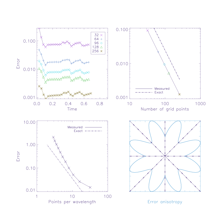
Figure 1: Errors in maintaining a divergenceless magnetic field as defined by equation (19). On the upper left panel is the error in the $L_{2}$ norm plotted as a function of time; note that there is an initial transient in the magnetic field, due to the applied current, followed by a period where the error undergoes some fluctuations. On the upper-right panel, the error as a function of grid spacing in the $L_{2}$ norm is plotted, along with a nominal second-order convergence rate curve. For a given calculation ($n_{x}=32$ here), the error is Fourier-decomposed and plotted as a function of wavenumber or equivalently, points per wavelength on the lower-left panel. The nominal line is also plotted, but the error is seen to only approximately fall at a second-order rate. Lastly, the error is anisotropic, as shown on the lower-right panel. Distance from the coordinate center denotes error magnitude; waves propagating at 22.5^∘ with respect to the axes are seen to be more inaccurately resolved than in other directions. This is a function of the choice of lattice and, in principle, error anisotropy may be reduced through the use of higher-order lattices.

4.2 Heterogeneous media

Next, we simulate wave propagation in an inhomogeneous medium, with the initial condition $B_{x}=(y-0.35)f(x,y)$, $B_{y}=-(x-0.5)f(x,y)$, where $f(x,y)=10\exp\left\{-[(x-0.5)^{2}+(y-0.35)^{2}]/(2\times 0.04^{2})\right\}$. As may be seen on the lower-left panel of Figure 2, the shape, size and magnitude of dielectric “defects” in this calculation bear a qualitative resemblance with the intermediate matched-impedance zero-index material region (MIZIM) discussed in [16]. However, different from [16], who consider frequency-dependent permittivity (implying a convolution with electric field), we only consider the time-stationary case. Also, we do not include inlet and outlet vacuum regions, but implement periodic boundary conditions. In order to avoid finite-size effects due to recirculating waves, the simulation is terminated before waves reach boundaries.

The initial Gaussian wave-packet splits into up- and downward propagating components. Waves of finite spatial extent refract into (away from) regions of low (high) $c$, because the portion of the waveform within the inhomogeneity propagates comparatively slower (faster). Moreover, since we study linear waves, wave frequency may be regarded as invariant, so that wavelength $\lambda\propto c$. Consequently, waves exhibit locally smaller (larger) wavelengths in regions of low (high) $c$. This implies that energy, defined as ${\mathcal{E}}=\sum_{\alpha}(B^{2}_{\alpha}+E^{2}_{\alpha}/c^{2})$, tends to concentrate in regions of low $c$, because waves spend larger fractions of time in these areas. The $(x,y)$ components of the Poynting energy-flux vector, ${\mathcal{P}}_{\alpha}=\epsilon_{\alpha\beta\gamma}E_{\beta}B_{\gamma}$, and electric field $E_{z}$ are also shown. These interpretations are confirmed by visual inspection of properties of the wavefield and $c^{2}({\bf x})$, as shown in Figures 2 and 3. Note that the magnitude of $c^{2}$ in vacuum is necessarily greater than the largest value in this medium. The refractive index, $n\propto c^{-1}$, is seen to vary by a factor of four ($c^{2}\sim 0.1-1.6$), comparable to contrasts used in [16] to fine-tune transmission (reflection) coefficients across the MIZIM region.

In order to test the accuracy of the LB solution, we repeat this calculation using a pseudo-spectral solver, in which spatial derivatives are computed spectrally and time stepping is achieved through the application of an optimized Runge-Kutta scheme [19]. In Figure 2, we also show a comparison between outputs of the two simulations. Grids in both solvers contain $512\times 512$ points; LB and pseudo-spectral solutions are very similar, with a 0.6% $L_{2}$ norm of the difference. The LB calculation at this resolution is approximately 4 times faster than its pseudo-spectral counterpart; however, these codes were not written with optimization and efficiency in mind and the number may only be interpreted loosely.

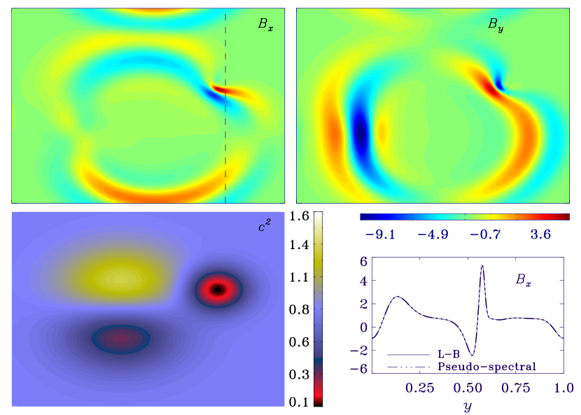
Figure 2: Upper panels show snapshots of $B_{x}$ and $B_{y}$ at $t=1.272$, with the initial condition described in the text; the lower left shows the spatial distribution of $c^{2}$. Axes of the three contour plots are $x$ and $y$. In both calculations, the grid contained $512\times 512$ points and the domains were horizontally periodic, with $x,y\in[0,1)$. The horizontal colorbar applies to the upper panels while the vertical bar describes the range in $c^{2}$. Regions of low wave-speed (compared with reference $c^{2}=1$; note that $c^{2}>1$ in vacuum, although we do not specify a value, since vacuum regions are not included in the computational domain) cause waves to refract towards them and vice-versa. The lower-right panel compares pseudo-spectral and LB solutions along a cut at constant $x$ (location indicated by the dashed line in the $B_{x}$ plot). The technique is seen to accurately simulate wave propagation through regions where refractive index $n~{}(\propto c^{-1})$ shows substantial local variations. The $L_{2}$ norm of the difference between LB and pseudo-spectral solutions is 0.6%. In order to prevent boundary periodicity from affecting the results, a larger computational domain may be chosen and the calculation terminated before waves reach the boundaries.

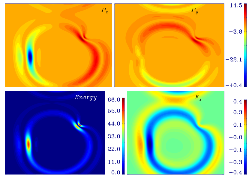
Figure 3: Upper panels show the $x-y$ components of Poynting vector, and lower panels display energy and electric field $E_{z}$. Axes of all plots are $x$ and $y$, on a periodic grid of $512\times 512$ points and $x,y\in[0,1)$. Since waves spend more time in regions of low wave-speed (shorter wavelengths), energy appears to be concentrated in these areas. The top-right scale applies to both upper panels.

5 Outlook

In summary, we demonstrate that top-down-prescribed distribution functions of “particles”, not based on any known microscopic kinetic theory of EM, succeed in reproducing the behavior predicted by the Maxwell equations. Moreover, our result provides a further example of lattice kinetic theory as an efficient tool to simulate continuum-physics phenomena via a particle-like formalism, well suited to handling complex geometries and showing excellent scalability on modern parallel computers [18]. The present method may be extended in many directions, such as invisibility cloaks, i.e., systems wherein the use of meta-materials allows for selected regions of space to become inaccessible to light, analogous to metric holes in space-time (e.g., Fig. 3 in [17]). Another possibility is to extend it to study plasma phenomena in confined geometries.

We note potential limitations of this technique and describe directions for future work. Like most LB methods, the present scheme is formulated in a space-time uniform lattice, so that space and time resolution may not be changed independently unless locally-adaptive formulations of the method are put in place. Such adaptive LB formulations do indeed exist [21], although they are usually significantly more laborious than the native version on uniform lattices. A second point regards numerical stability in the presence of sharp interfaces, resolved by just a few lattice points. At such sharp interfaces, higher order terms may no longer be negligible, thereby introducing unwanted dissipative effects. Efficient implementations with non-local permittivities, as mentioned earlier on in this paper, are likely to require a careful analysis of the auxiliary equations to be coupled with the native LB equation for waves. This is similar to the way auxiliary equations are coupled to the LB equation for the modeling of turbulent fluid flows [22].

The present LB scheme may be regarded as a special type of finite-difference method, in which streaming is exact and local conservations are built-in and accurate to machine round-off. Although the technique is just second-order in space-time, the above properties make the error prefactors sufficiently small so as to render its performance competitive with higher-order methods, including spectral ones.

From a mathematical stand point, the inclusion of source terms, reflecting external sources and/or inhomogeneities, is straightforward, once the expression of these sources in the continuum is known. However, the strengths of such terms may place stringent constraints on the stability of the scheme, aspects that remain to be investigated.

Although we have only considered periodic boundaries, we note that there exists literature on the implementation of other boundary conditions, such as reflecting, absorbing etc. (e.g., [3] and references therein) As a result, the formulation of different types of boundary conditions for the wave-LB scheme might follow from previous developments although such a possibility remains to be studied in full detail.

Despite their importance, the above developments that do not challenge the basic merits of the scheme discussed in this paper. As a result, we believe that the LB scheme presented in this work should offer a fast and flexible computational tool to assist, complement and possibly even anticipate experimental research on invisibility cloaks and related phenomena in modern optics and photonics research [23, 24].

- [1] P. Bhatnagar et al., Phys. Rev. 94, 511, (1954).
- [2] R. Benzi et al., Phys. Rep. 222, 145, (1992).
- [3] C. K. Aidun and J. R. Clausen, Annu. Rev. Fluid Mech., 42, 439, (2010).
- [4] M. Mendoza et al., Phys. Rev. Lett., 105, 014502, (2010).
- [5] M. Wegener and S. Linden, Phys. Today, 63, 32, (2010).
- [6] P. Mora, J. Stat. Phys., 68, 591, (1992).
- [7] B. Chopard and M. Droz, Cellular Automata Modelling of Physical Systems, Cambridge U.P., (1998).
- [8] Y. Guangwu, J. Comp. Phys., 161, 61, (2000).
- [9] Marconi, Int. J. Mod. Phys. B, 17, 153-156, (2003)
- [10] M. Mendoza and J.D. Munoz, Phys. Rev. E, 77, 026713, (2008).
- [11] M. Mendoza and J.D. Munoz, Phys. Rev. E, 82, 056708, (2010).
- [12] P. Dellar, J. Stat. Mech., P06003, (2009).
- [13] P. Dellar, EPL, 90, 50002, (2010).
- [14] A. Taflove and S. Hagness, “Computational Electrodynamics: The Finite-Difference Time-Domain Method”, Third Edition, Artech House, (2005).
- [15] E. Barouch, S. L. Knodle and S. A. Orszag, “Computation of Broadband Electromagnetic Direct and Inverse Scattering with Non-Linear Lossy Targets. I. Material Properties”, J. Sci. Comp. sub judice, (2011).
- [16] V. C. Nguyen et al., Phys. Rev. Lett., 105, 233908, (2010).
- [17] M. Wegener and S. Linden, Phys. Today, 63, 32, (2010).
- [18] Challenges in simulating wave propagation in complex geometries are well described in I. Simonsen et al., Phys. Rev. Lett., 104, 223904, (2010).
- [19] F. Q. Hu et al., J. Comp. Phys. 124, 177, (1996).
- [20] D. W. Gladrow, “Lattice-gas cellular automata and lattice Boltzmann models: an introduction”, Springer Verlag, (2000); S. Succi, “The Lattice-Boltzmann Equation for Fluid Dynamics and Beyond”, Oxford Univ. Press, (2001); M. Sukop and D. Thorne, Lattice Boltzmann Modeling: An Introduction for Geoscientists and Engineers, Springer Verlag, (2007).
- [21] S. Succi, O. Filippova, G. Smith et al. Computing in Science and Engineering, 3, 26, (2001); B. Crouse, E. Rank, M. Krafczyk M, et al. Int. J. Mod. Phys. B, 17, 109, (2003).
- [22] H. Chen, S. Kandasamy, S. Orszag et al., Science, 301, 633, (2003).
- [23] J.B. Pendry et al., Science, 312, 1780, (2006).
- [24] J. Li and J.B. Pendry, Phys. Rev. Lett., 101, 203901, (2008).