Measuring large-scale structure with quasars in narrow-band filter surveys

Abstract

We show that a large-area imaging survey using narrow-band filters could detect quasars in sufficiently high number densities, and with more than sufficient accuracy in their photometric redshifts, to turn them into suitable tracers of large-scale structure. If a narrow-band optical survey can detect objects as faint as $i=23$, it could reach volumetric number densities as high as $10^{-4}\,h^{3}$ Mpc^-3 (comoving) at $z\sim 1.5$. Such a catalog would lead to precision measurements of the power spectrum up to $z\sim 3-4$. We also show that it is possible to employ quasars to measure baryon acoustic oscillations at high redshifts, where the uncertainties from redshift distortions and nonlinearities are much smaller than at $z\lesssim 1$. As a concrete example we study the future impact of J-PAS, which is a narrow-band imaging survey in the optical over 1/5 of the unobscured sky with $42$ filters of $\sim 100$ Å full-width at half-maximum. We show that J-PAS will be able to take advantage of the broad emission lines of quasars to deliver excellent photometric redshifts, $\sigma_{z}\simeq 0.002\,(1+z)$, for millions of objects.

1 Introduction

Quasars are among the most luminous objects in the Universe. They are believed to be powered by the accretion disks of giant black holes that lie at the centers of galaxies [Salpeter (1964); Zel’Dovich & Novikov (1965); Lynden-Bell (1969)], and the extreme environments of those disks are responsible for emitting the “non-stellar continuum” and the broad emission lines that characterize the spectral energy distributions (SEDs) of quasars and most other types of Active Galactic Nuclei (AGNs).

However, even though all galaxy bulges in the local Universe seem to host supermassive black holes in their centers [Kormendy & Richstone (1995)], the duty cycle of quasars is much smaller than the age of the Universe [Richstone et al. (1998)]. This means that at any given time the number density of quasars is small compared to that of galaxies.

As a consequence, galaxies have been the preferred tracers of large-scale structure in the Universe: their high densities and relatively high luminosities allow astronomers to compile large samples, distributed across vast volumes. Both spectroscopic [see, e.g., Cole et al. (2005); York et al. (2000); BOSS] and broad-band (e.g., $ugriz$) photometric surveys [Scoville et al. (2007); Adelman-McCarthy et al. (2008a, b)] have been used with remarkable success to study the distribution of galaxies, particularly so for the subset of luminous red galaxies (LRGs), for which it is possible to obtain relatively good photometric redshifts (photo-z’s) [$\sigma_{z}\sim 0.01\,(1+z)$] even with broad-band filter photometry [Bolzonella et al. (2000); Benítez (2000); Firth et al. (2003); Padmanabhan et al. (2005, 2007); Abdalla et al. (2008a, b, c)]. From a purely statistical perspective, photometric surveys have the advantage of larger volumes and densities than spectroscopic surveys – albeit with diminished spatial resolution in the radial direction, which can be a limiting factor for some applications, in particular baryon acoustic oscillations (BAOs) [Blake & Bridle (2005)].

Most ongoing wide-area surveys choose one of the parallel strategies of imaging [e.g., Abbott et al. (2005); PAN-STARRS;Abell (2009)] or multi-object spectroscopy (e.g., BOSS), and future instruments will probably continue following these trends, since spectroscopic surveys need wide, deep imaging for target selection, and imaging surveys need large spectroscopic samples as calibration sets.

However, whereas LRGs possess a signature spectral feature (the so-called $\lambda_{\rm rest}\sim$ 4,000 Å break), which translates into fairly good photo-z’s with $ugriz$ imaging, the SEDs of quasars observed by broad-band filters only show a similar feature (the Ly-$\alpha$ line) at $\lambda_{\rm rest}\sim$ 1,200 Å, which makes them UV-dropout objects. The segregation of quasars from stars and unresolved galaxies in color-color and color-magnitude diagrams has allowed the construction of a high-purity catalog of $\sim 1.2\times 10^{6}$ photometrically selected quasars in the SDSS [Richards et al. (2008)], and the (broad-band) photometric redshifts of $z<2.2$ objects in that catalog can be estimated by the passage of the emission lines from one filter to the next [Richards et al. (2001)]. More recently, Salvato et al. (2009) showed that a combination of broad-band and medium-band filters reduced the photo-z errors of the XMM-COSMOS sources down to $\sigma_{z}/(1+z)\sim 0.01$ (median).

The SDSS spectroscopic catalog of quasars [Schneider et al. (2003, 2007, 2010)] is five times bigger than previous samples [Croom et al. (2004)], but includes only $\sim 10$% of the total number of good candidates in the photometric sample. Furthermore, that catalog is limited to relatively bright objects, with apparent magnitudes $i\lesssim 19.1$ at $z<3.0$, and $i<20.2$ for objects with $z>3.0$. Despite the sparseness of the SDSS spectroscopic catalog of quasars (the comoving number density of objects in that catalog peaks at $\lesssim 10^{-6}$ Mpc^-3 around $z\sim 1$), it has been successfully employed in several measurements of large-scale structure – see, e.g., Porciani et al. (2004); da Ângela et al. (2005), which used the 2QZ survey [Croom et al. (2005, 2009b)] for the first modern applications of quasars in a cosmological context; see Shen et al. (2007); Ross et al. (2009) for the cosmological impact of the SDSS quasar survey; and Padmanabhan et al. (2008), which cross-correlated quasars with the SDSS photometric catalog of LRGs. One can also use quasars as a backlight to illuminate the intervening distribution of neutral H, which can then be used to compute the mass power spectrum [Croft et al. (1998); Seljak et al. (2005)].

The broad emission lines of type-I quasars [Vanden Berk et al. (2001)], which are a manifestation of the extremely high velocities of the gas in the environments of supermassive black holes, are ideal features with which to obtain photo-z’s, if only the filters were narrow enough ($\Delta\lambda\lesssim 400$ Å) to capture those features. In fact, Wolf et al. (2003b) have produced a sample of a few hundred quasars using a combination of broad-band and narrow-band filters (the COMBO-17 survey), obtaining a photo-z accuracy of approximately 3% – basically the same accuracy that was for their catalog of galaxies [Wolf et al. (2003a)]. Acquiring a sufficiently large number of quasars in an existing narrow-band galaxy survey would be both feasible and it would bear zero marginal cost on the survey budgets.

Fortunately, a range of science cases that hinge on large volumes and good spectral resolution, in particular galaxy surveys with the goal of measuring BAOs [Peebles & Yu (1970); Sunyaev & Zeldovich (1970); Bond & Efstathiou (1984); Holtzman (1989); Hu & Sugiyama (1995)], both in the angular [Eisenstein et al. (2005); Tegmark et al. (2006); Blake et al. (2007); Padmanabhan et al. (2007); Percival et al. (2007)] and in the radial directions [Eisenstein & Hu (1999); Eisenstein (2003); Blake & Glazebrook (2003); Seo & Eisenstein (2003); Angulo et al. (2008); Seo & Eisenstein (2007)] has stimulated astronomers to construct new instruments. They should be not only capable of detecting huge numbers of galaxies, but also of measuring much more precisely the photometric redshifts for these galaxies – and that means either low-resolution spectroscopy, or filters narrower than the $ugriz$ system.

Presently there are a few instruments which can be characterized either as narrow-band imaging surveys, or low-resolution multi-object spectroscopy surveys: the Alhambra survey [Moles et al. (2008)], PRIMUS [Cool (2008)], HETDEX and the PAU survey. The Alhambra survey uses the LAICA camera on the 3.5 m Calar Alto telescope, and is mapping 4 deg² between 3,500 Å and 9,700 Å, using a set of 20 filters equally spaced in the optical plus $JHK$ broad filters in the NIR. PRIMUS takes low-resolution spectra of selected objects with a prism and slit mask built for the IMACS instrument at the 6.5 m Magellan/Baade telescope. PRIMUS has already mapped $\sim$ 10 deg² of the sky down to a depth of 23.5, and has extracted redshifts of $\sim 3\times 10^{5}$ galaxies up to $z=1$, with a photo-z accuracy of order 1% [Coil et al. (2010)]. HETDEX is a large-field of view, integral field unit spectrograph to be mounted on the 10 m Hobby-Eberly telescope that will map 420 deg² with filling factor of 1/7 and an effective spectral resolution of 6.4 Å between 3,500 and 5,500 Å. The PAU survey will use 40 narrow-band filters and five broadband filters mounted on a new camera on the William Herschel Telescope to observe 100-200 deg² down to a magnitude $i_{AB}\sim 23$. All these surveys will detect large numbers of intermediate- to high-redshift objects (including AGNs), and by their nature will provide very dense, extremely complete datasets.

Another instrument which plans to make a wide-area spectrophotometric map of the sky is the Javalambre Physics of the Accelerating Universe Astrophysical Survey (J-PAS). The instrument [see Benítez et al. (2009)] will consist of two telescopes, of 2.5 m (T250) and 0.8 m (T80) apertures, which are being built at Sierra de Javalambre, in mainland Spain (40^o N) [Moles et al. (2010)]. A dedicated 1.2 Gpixel survey camera with a field of view of 7 deg² (5 deg² effective) will be mounted on the focal plane of the T250 telescope, while the T80 telescope will be used mainly for photometric calibration. The survey (which is fully funded through a Spain-Brazil collaboration) is planned to take 4-5 years and is expected to map between 8,000 and 9,000 deg² to a 5$\sigma$ magnitude depth for point sources equivalent to $i_{\rm AB}\sim 23$ ($i\sim 23.3$) over an aperture of 2 arcsec². The filter system of the J-PAS instrument, as originally described in Benítez et al. (2009), consists of 42 contiguous narrow-band filters of 118 Å FWHM spanning the range from 4,300 Å to 8,150 Å – see Fig. 1. This set of filters was designed to extract photo-z’s of LRGs with (rms) accuracy as good as $\sigma_{z}\simeq 0.003\,(1+z)$. Of course, this filter configuration is also ideal to detect and extract photo-z’s of type-I quasars – see Fig. 2.

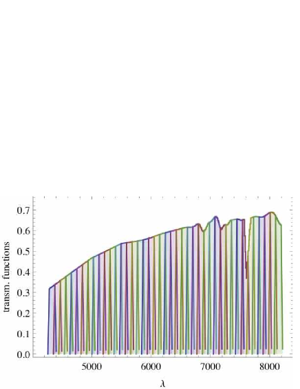
Figure 1: Throughputs of the original J-PAS filter system, assuming an airmass of 1.2, two aluminum reflections and the quantum efficiency of the LBNL CCDs (N. Benítez, private communication). The 42 narrow-band filters are spaced by 93 Å, with 118 Å FWHM, and span the interval between 4,250 Å and 8,200 Å. The final filter system for J-PAS is still under review, and may present small deviations from the original filter set of Beníitez et al. (2009) – see Beníitez et al. (2011), to appear. We have checked that the results presented in this paper are basically insensitive to these small variations.

Figure 2: Three SDSS quasars as they would be observed by the filter system of Fig. 1. The SDSS objects are, from top to bottom: J000143.41-152021.4 ($z=2.638$), J001138.43-104458.2 (at $z=1.271$), and J002019.22-110609.2 ($z=0.492$). The light (blue in color version) curve indicates the flux (in units of $10^{-17}$ erg/s/cm²/Å) in spectral bins of the original SDSS spectra; the large (red) dots denote the corresponding fluxes (normalized by the filter throughput) for the J-PAS narrow-band filters. Some emission lines can be seen in the photometric data: Ly-$\alpha$, Si IV, C IV and C III] for the spectrum on top; C III] and Mg II for the quasar in the central panel; and Mg II, H$\gamma$ and H$\beta$ (together with the [O III] doublet) for the spectrum on the bottom.

In this paper we show that a narrow-band imaging survey such as J-PAS will detect quasars in sufficiently high numbers ($\sim 2.\times 10^{6}$ up to $z\simeq 5$), and with more than sufficient redshift accuracy, to make precision measurements of the power spectrum. In particular, these observations will yield a high-redshift measurement of BAOs, at an epoch where redshift distortions and nonlinearities are much less of a nuisance than in the local Universe. This huge dataset may also allow precision measurements of the quasar luminosity function [Hopkins et al. (2007)], clustering and bias [Shen et al. (2007); Ross et al. (2009); Shen et al. (2010)], as well as limits on the quasar duty cycle [Martini & Weinberg (2001)].

This paper is organized as follows: In Section II we show how narrow ($\sim 100$ Å bandwidth) filters can be used to extract redshifts of quasars with high efficiency and accuracy. We compare two photo-z methods: empirical template fitting, and the training set method. Still in Section II, we study the issues of completeness and contamination. In Section III we compute the expected number of quasars in a flux-limited narrow-band imaging survey, and derive the uncertainties in the power spectrum that can be achieved with that catalog. Our fiducial cosmological model is a flat $\Lambda$CDM Universe with $h=0.72$ and $\Omega_{m}=0.25$, and all distances are comoving, unless explicitly noted.

As we were finalizing this work, a closely related preprint, Sawangwit et al. (2011), came to our notice. In that paper the authors analyze the SDSS, 2QZ and 2SLAQ quasar catalogs in search of the BAO features – see also Yahata et al. (2005) for a previous attempt using only the SDSS quasars. Although Sawangwit et al. are unable to make a detection of BAOs with these combined catalogs, they have forecast that a spectroscopic survey with a quarter million quasars over 2000 deg² would be sufficient to detect the scale of BAOs with accuracy comparable to that presently made by LRGs – but at a higher redshift. Their conclusions are consistent with what we have found in Section III of this paper.

2 Photometric redshifts of quasars

The idea of using the fluxes observed through multiple filters, instead of full-fledged spectra, to estimate the redshifts of astronomical objects, is almost five decades old [Baum (1962)], but only recently it has acquired greater relevance in connection with photometric galaxy surveys [Connolly et al. (1995); Bolzonella et al. (2000); Benítez (2000); Blake & Bridle (2005); Firth et al. (2003); Budavári (2009)]. In fact, many planned astrophysical surveys such as DES [Abbott et al. (2005)], Pan-STARRS and the LSST [Abell (2009)] are relying (or plan to rely) almost entirely on photometric redshifts (photo-z’s) of galaxies for the bulk of their science cases.

Photometric redshift methods can be divided into two basic groups: empirical template fitting methods, and training set methods – see, however, Budavári (2009) for a unifying scheme. With template-based methods [which may include spectral synthesis methods, e.g. Bruzual & Charlot (2003)] the photometric fluxes are fitted (typically through a $\chi^{2}$) to some model, or template, which has been properly redshifted, and the photometric redshift (photo-z) is given by a maximum likelihood estimator (MLE). In the training set approach, a large number of spectra is used to empirically calibrate a multidimensional mapping between photometric fluxes and redshifts, without explicit modeling templates.

The performance of template fitting methods and of training set methods are similar when they are applied to broad-band photometric surveys [Budavári (2009)]. In this paper we have taken both approaches, in order to compare their performances specifically for the case of a narrow-band filter surveys of quasars.

2.1 The spectroscopic sample of quasars

We have randomly selected a sample of 10,000 quasars from the compilation of Schneider et al. (2010) of all spectroscopically confirmed SDSS quasars, that lie in the Northern Galactic Cap, that have an i-band magnitude brighter than 20.4, and that have low Galactic extinction, as determined by the maps of Schlegel et al. (1998). Avoiding the Southern Galactic Cap means that the sample does not contain the various “special” samples of quasars targeted on the Celestial Equator in the Fall sky [Adelman-McCarthy et al. (2006)], which tend to be more unusual, fainter, or less representative of the quasar population as a whole. The magnitude limit also removes those objects at lowest signal-to-noise ratio. Indeed, the vast majority of the $10^{4}$ objects are selected using the uniform criteria described by Richards et al. (2002). The SEDs of these objects were measured in the interval 3,793 Å $<\lambda<$ 9,221 Å, with a spectral resolution of $R\simeq$ 2,000 and accurate spectrophotometry [Adelman-McCarthy et al. (2008b)]. The number of quasars as a function of redshift in our sample is shown in the left (red in color version) bars of Fig. 3, and reproduces the redshift distribution of the SDSS quasar catalog as a whole rather well.

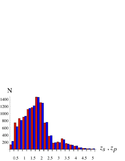
Figure 3: Redshift distribution of our full sample of quasars, in terms of their spectroscopic redshifts $z_{s}$ (left bars, red in color version) and their photometric redshifts $z_{p}$ obtained through the template fitting method of Section 2.3 (right bars, blue in color version), in bins of $\Delta z=0.25$. Left panel: sub-sample of SDSS quasars; right panel: simulated sample of fainter objects.

Starting from the spectra of our sample, we constructed synthetic fluxes using the 42 transmission functions shown in Fig. 1. The reduction is straightforward: the flux is obtained by the convolution of the SDSS spectra with the filter transmission functions:

$$f_{a(p)}=\frac{1}{n_{a}}\int T_{a}(\lambda)S_{p}(\lambda)d\lambda\;,$$

where $f_{a(p)}$ is the flux of the object $p$ measured in the narrow-band filter $a$, $T_{a}$ is the transmission function of the filter $a$, $n_{a}=\int T_{a}(\lambda)d\lambda$ is the total transmission normalization, and $S_{p}$ is the SED of the object. The noise in each filter in obtained by adding the noise in each spectral bin in quadrature.

2.2 Simulated sample of quasars

The procedure outlined above generates fluxes with errors which are totally unrelated to the errors we expect in a narrow-band filter survey. The magnitude depths (and the signal-to-noise ratios) of the original SDSS sample are characteristics of that instrument, and corresponds to objects with $i<19.1$ for $z<3.0$, and $i<20.2$ for $z>3$. However, we want to determine the accuracy of photo-z methods for a narrow-band survey that reaches $i\sim 23$. Hence, we need a sample which includes, on average, much less luminous objects than the SDSS catalog does. It is easy to construct an approximately fair sample of faint objects from a fair sample of bright objects, as long as the SEDs of these objects do not depend strongly on their luminosities – which seems to be the case for quasars [Baldwin (1977)].

We have used our original sample of 10,000 SDSS quasars described in the previous Section to construct a simulated sample of quasars. For each object in the original sample with a magnitude $i$ we associate an object in the simulated sample of magnitude $i_{s}$, given by:

$$i_{s}=14+1.5(i-14)\;.$$ (1)

Since the original sample had objects with magnitudes $i\sim 14-20.5$, the simulated sample has objects ranging from $i_{s}\sim 14$ to $i_{s}\sim 23.5$. The distribution of quasars as a function of their magnitudes, in the original and in the simulated samples, are shown in Fig. 4. Clearly, Eq. (1) still reproduces the selection criteria of the original SDSS sample, which is evidenced by the step-like features of the histograms shown in Fig. 4. However, in this Section we are not as concerned with the number of quasars as a function of redshift and magnitude (which we believe are well represented by the luminosity function that was employed in the previous Section), but with the accuracy of the photometric redshifts and the fraction of catastrophic outliers – i.e., the instances when the photometric redshifts deviate from the spectroscopic redshifts by more than a given threshold. While we have not detected any significant correlations between the absolute or relative magnitudes and the accuracy of the photo-z’s, we have found that the number of photo-z outliers is higher for the simulated sample, compared with the original sample, which means that the rate of outliers does depend to some extent on the actual magnitudes of the sample. This is discussed in detail in Section 2.3.

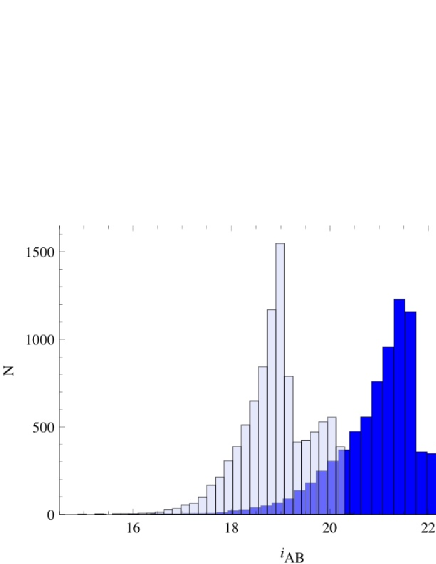
Figure 4: Distribution of magnitudes of the objects in our original sample (light bars) and in the simulated sample (dark bars.)

In order to generate realistic signal-to-noise ratios (SNR) for the objects in this simulated sample, we also need to specify the depths of the survey that we are considering, in each one of its 42 filters. The 5$\sigma$ magnitude limits that we have estimated for J-PAS, considering the size of the telescope, an aperture of 2 arcsec, the median seeing at the site, the total exposure times for an 8,000 deg² survey over 4 years, the presumed read-out noise, filter throughputs, night sky luminosity, lunar cycle, etc., are shown in Fig. 5.

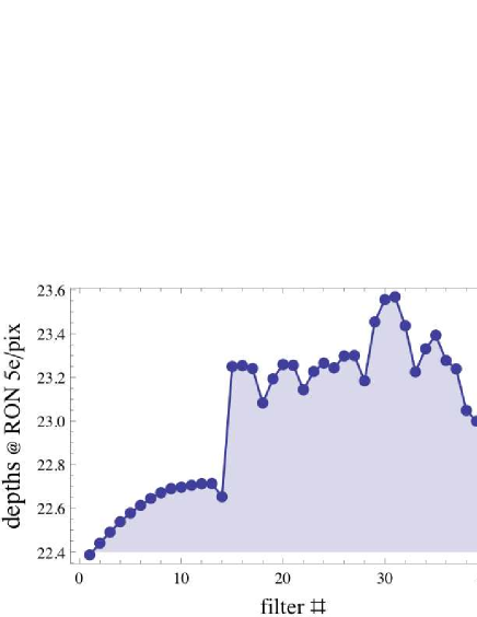
Figure 5: Estimated limiting magnitudes ($5\sigma$) for J-PAS with an aperture of 2”, assuming a read-out noise of 5e/pixel.

Our model for the signal-to-noise ratio (SNR) in each filter, for simulated quasars of a given i-band magnitude $i_{s}$, is the following:

$$SNR(a)=5\,\frac{f(a)}{\bar{f}_{i}}\,10^{0.4[d(a)-i_{s}]}\;,$$ (2)

where $\bar{f}_{i}$ is the average flux of that object in the 10 filters (7,100 $\leq\lambda\leq$ 8,100) that overlap with the $i$-band; $f(a)$ is the flux in filter $a$; $d(a)$ is the $5\sigma$ depth of filter $a$ from Fig. 5; and $i_{s}$ is the (simulated) $i$-band magnitude of that object. This model assumes that the intrinsic photon counting noise of the quasar is subdominant compared to other sources of noise such as the sky or the host galaxy. In order to obtain the desired SNR in our simulated sample, we have added a white (Gaussian) noise to the fluxes of the original sample, such that the final level of noise is the one prescribed by Eq. (2).

2.3 Photometric redshifts of quasars: Template Fitting Method

Conceptually, fitting a series of photometric fluxes to a template is the simplest method to obtain redshifts from objects that belong to a given spectral class [Benítez (2000)]. Type-I quasars possess a (double) power-law continuum that rises rapidly in the blue, and a series of broad ($\Delta\lambda/\lambda\sim$ 1/20 – 1/10 FWHM) emission lines – see Fig. 2. At high redshifts ($z\gtrsim 2.5$) the Ly-$\alpha$ break (which is a sharp drop in the observed spectrum of distant quasars due to absorption from intervening neutral Hydrogen) can be seen at $\lambda\gtrsim$ 4,000 Å, which lies just within the dynamic range of the filter system we are exploring here. These very distinct spectral features, which are clearly resolved with our filter system, allow not only the extraction of excellent photo-z’s, but can also be used to distinguish quasars from stars unambiguously – see, e.g., the SDSS spectral templates, Adelman-McCarthy et al. (2008a). The COMBO-17 quasar catalog [Wolf et al. (2003b)] has successfully employed a template fitting method not only to obtain photometric redshifts, but also to identify stars and understand the completeness and rate of contamination of the quasar sample.

Here we will assume that all quasars have already been identified, and the only parameter that we will fit in our tests is the redshift of a given object. A more detailed analysis will be the subject of a forthcoming publication (Gonzalez-Serrano et al., 2012, to appear).

Our baseline model for the quasar spectra is the Vanden Berk mean template [Vanden Berk et al. (2001)], which also includes the uncertainties due to intrinsic variations. We allow for further variability in the quasar spectra by means of the global eigen-spectra computed by Yip et al. (2004). We use both the uncertainties in the Vanden Berk template and the Yip et al. eigen-spectra because they capture different types of intrinsic variability: while the uncertainties in the template are more suited to allow for uncorrelated variations around the emission lines and below the Ly-$\alpha$, the Yip et al. eigen-spectra allow for features such as contamination from the host galaxy (which is most relevant at low luminosities), UV-optical continuum variations, correlated Balmer emission lines and other secondary effects such as broad absorption line systems. We search for the best-fit combination of the four eigen-spectra at each redshift, by varying their weights ($w_{p,z}$ , $p=1\cdots 4$) in the interval $-3w_{p}\leq w_{p,z}\leq 3w_{p}$, where $w_{p}$ is the weight of the $p$-th eigenvalue relative to the mean. The four highest-ranked global eigen-spectra have weights of $w_{1}=0.119$, $w_{2}=0.076$, $w_{3}=0.066$, and $w_{4}=0.028$ relative to the mean template spectrum (which has $w_{0}=1$ by definition) [Yip et al. (2004)].

The eigen-spectra are included in the MLE in the following way: first, we normalize the fluxes by their square-integral, i.e.: $f_{a}\rightarrow f^{n}_{a}=f_{a}/\sqrt{\sum_{b=1}^{N}f_{b}^{2}}$, where $N$ is the number of filters (42 for J-PAS.) We then add the redshifted eigen-spectra $f^{n}_{p,a}(z)$ to the average template [$f^{n}_{0,a}(z)$] with weights $w_{p}(z)$, so that at each redshift we have $f_{a}^{n}=f^{n}_{0,a}+\sum_{p=1}^{4}w_{p}f^{n}_{p,a}$. The weights $w_{p}$ are found by minimizing the (reduced) $\chi^{2}$ at each redshift:

$$\chi^{2}(i,z)=\frac{1}{N}\sum_{a}^{N}\frac{\left[f_{a}^{n}-f_{a}^{n}(i)\right]^{2}}{\sigma_{a}^{2}(i,z)}\;,$$ (3)

where $f_{a}^{n}(i)$ are the fluxes from some object $i$ in our sample of SDSS quasars, and $\sigma_{a}^{2}(i,z)$ is the sum in quadrature of the flux errors and of the (2-$\sigma$) uncertainties in the quasar template spectrum for that filter. We have not marginalized over the weights of the eigen-spectra – i.e., the method is indifferent as to whether or not the best fit to an object at a given redshift includes an unusually large contribution from some particular eigen-mode.

It is also interesting to search for the linear combination between the fluxes that leads to the most accurate photo-z’s. We could have employed either the fluxes themselves or the colors (flux differences) for the procedure that was outlined above – or, in fact, any linear combination of the fluxes. Most photo-z methods employ colors [Benítez (2000); Blake & Bridle (2005); Firth et al. (2003); Budavári (2009)], since this seems to reduce the influence of some systematic effects such as reddening, and it also eliminates the need to marginalize over the normalization of the observed flux. We have tested the performance of the template fitting method using the fluxes $f_{a}$, the colors $\Delta f_{a}=f_{a}-f_{a-1}$ (the derivative of the flux), and also the second differences $\Delta^{2}f_{a}=f_{a+1}-2f_{a}+f_{a-1}$ (the second derivative of the flux, or color differences.) We have noticed a slightly better performance with the latter choice ($\Delta^{2}f_{a}$) when compared with the usual colors ($\Delta f_{a}$), but the difference is negligible and therefore in this work we have kept the usual practice of using colors. The results shown in the remainder of this Section refer to the traditional template-fitting method with colors.

In Fig. 6 we plot the distribution of $\log_{10}\chi^{2}$ (for the best-fit $\chi^{2}$ among all $z$’s) for our sample of $10^{4}$ quasars. The wide variation in the quality of the fit is partly due to the small number of free parameters: we fit only the redshift and the weights of the four eigen-modes.

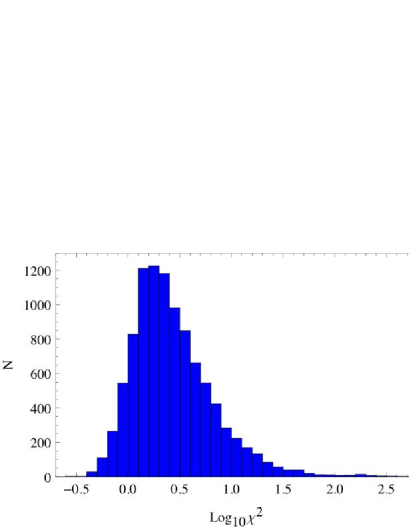
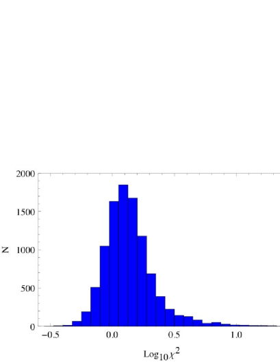
Figure 6: Histogram of the best-fit reduced $\chi^{2}$ for the sample of $10^{4}$ quasars from the SDSS spectroscopic catalog. Left panel: original SDSS sample limited at $i\lesssim 20.1$; right panel: simulated sample, effectively limited at $i\lesssim 23.5$. We point out that the distributions above are not at all typical of a $\chi^{2}$ probability distribution function – the horizontal axis is in fact $\log_{10}\chi^{2}$.

Once the $\chi^{2}(z)$ has been determined for a given object, we build the corresponding posterior probability distribution function (p.d.f.):

$$p(z)\propto e^{-\chi^{2}(z)/2}\;.$$ (4)

The photometric redshift is the one that minimizes the $\chi^{2}$ (the MLE.)

Finally, we need to estimate the “odds” that the photo-z of a given object is accurate. Due to the many possible mismatches between different combinations of the emission lines, the p.d.f.’s are highly non-Gaussian, with multiple peaks (i.e., multi-modality.) Hence, we have employed an empirical set of indicators to assess the quality of the photo-z’s. These empirical indicators are: (i) the value of the best-fit $\chi^{2}$; (ii) the ratio between the posterior p.d.f. $p(z)$ at the first (global) maximum of the p.d.f. and the value of the p.d.f. at the secondary maximum (if it exists), $r=p_{max\#1}/p_{max\#2}$; and (iii) the dispersion of the p.d.f. around the best fit, $\sigma=\int(z-z_{best})^{2}p(z)dz$. We then maximize the correlation between the redshift error $|z_{p}-z_{s}|/(1+z_{s})$ and a linear combination of simple functions of these indicators. Finally, we normalize the results so that they lie between $0$ (a very bad fit) and $1$ (very good fit.)

For the original SDSS sample, we found empirically that the combination that correlates (positively) most strongly with the photo-z errors (the quality) is given by:

$${\rm q}=0.15\log(0.7+\chi^{2}_{bf})+e^{8(r-1)}+0.06\,e^{1.4\sigma}\;.$$ (5)

For the simulated sample, the quality indicator is:

$${\rm q}=0.3\log(0.6+\chi^{2}_{bf})+e^{15(r-1)}+0.026\,e^{\sigma}\;.$$ (6)

Finally, we compute the quality factor $0<\bar{q}\leq 1$ with the formula:

$$\bar{q}=\left[\frac{{\rm max}(q)-q}{{\rm max}(q)-{\rm min}(q)}\right]^{4}\;,$$ (7)

where the power of $4$ was introduced to produce a “flatter” distribution of bad and good fits (this step does not affect the photo-z quality cuts that we impose below).

The relationship between the quality factor and the photometric redshift errors is shown in the distributions of Fig. 7. There is a strong correlation between the quality factor and the rate of “catastrophic errors”, which we define arbitrarily as any instance in which $|z_{p}-z_{s}|/(1+z_{s})\geq 0.02$ – denoted as the horizontal dashed lines in Fig. 7. We have adopted the usual convention of scaling the redshift errors by $1+z$, since this is the scaling of the rest-frame spectral features. There is no obvious reason why emission-line systems (whose salient features can enter or exit the filter system depending on the redshift) should also be subject to this scaling, but we have verified that the scatter in the non-catastrophic photo-z estimates do indeed scale approximately as $1+z$.

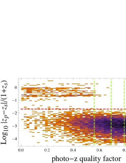
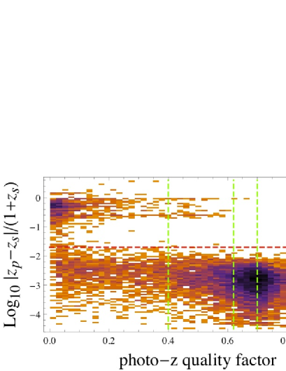
Figure 7: 2D histograms of the photo-z errors $\log_{10}|z_{p}-z_{s}|/(1+z_{s})$ (vertical axis) and the quality factor $\bar{q}$ (horizontal axis). The left and right panels correspond to the original and the simulated samples, respectively. The catastrophic redshift errors [$|z_{p}-s_{s}|/(1+z_{s})\geq 0.02$] lie above the horizontal dashed (red in color version) line. The quality factor has been grouped into four “grades”, from grade=1 to grade=4, according to the vertical dashed (green in color version) lines.

We have divided our sample into four groups with an equal number of objects, according to the value of $\bar{q}$: lowest quality ($g_{1}$, 2,500 objects), medium-low quality ($g_{2}$, 2,500 objects), medium-high quality ($g_{3}$, 2,500 objects) and highest quality ($g_{4}$, 2500 objects) photo-z’s. These grade groups are separated by the vertical dotted lines shown in Fig. 7. For the original sample, the rate of catastrophic redshifts is 16.9 %, 0.08 %, 0 % and 0 % in the grade groups $g_{1}$, $g_{2}$, $g_{3}$ and $g_{4}$, respectively. For the simulated sample, the rate of catastrophic errors is 44.7 %, 2.3 %, 0.001 % and 0 % in the groups $g_{1}$, $g_{2}$, $g_{3}$ and $g_{4}$, respectively.

The relationship between spectroscopic and photometric redshifts is shown in Fig. 8, where each quadrant corresponds to a grade group. Almost all the catastrophic redshift errors are in the $g_{1}$ grade group, and most of the catastrophic errors lie below $z_{p}\lesssim 2.5$ – since it is above this redshift that the Ly-$\alpha$ break becomes visible in our filter system.

From Figs. 7 and 8 it is clear that the rate of catastrophic photo-z’s is larger for the simulated sample, which has an overall fraction of approximately 12% of outliers, compared to the original sample, which has a total fraction of 4% of outliers. A similar increase happens also when the Training Set method is applied to these samples (see the next Section). Since the simulated sample used in this Section was not designed to reproduce the actual distribution of magnitudes expected in a real catalog of quasars, this means that our results for the rate of outliers are only an estimate for the actual rate that we should expect from the final J-PAS catalog. However, even as the rate of outliers increases from the original to the simulated samples, the accuracy of the photo-z’s are still very nearly the same. This means that the actual distribution of magnitudes of an eventual J-PAS quasar catalog should have little impact on the accuracy of the photo-z’s – although it could affect the completeness and purity of that catalog.

A further peculiarity of the quasar photo-z’s is evident in the lines $z_{p}=z_{*}+\alpha z_{s}$, which are most prominent in the $g_{1}$ groups of the original and simulated samples, as well as the $g_{2}$ group of the simulated sample. Whenever two (or more) pairs of broad emisson lines are separated by the same relative interval in wavelength, i.e. $\lambda_{\alpha}/\lambda_{\beta}\simeq\lambda_{\gamma}/\lambda_{\delta}$, (where $\lambda_{\alpha\cdots\delta}$ are the central wavelengths of the emission lines), there is an enhanced potential for a degeneracy of the fir between the data and the template – i.e., additional peaks appear in the p.d.f. $p(z)$. As the true redshift of the quasar change, the ratios between these lines remain invariant, and so the ratios between the true and the false redshifts, $(1+z_{true})/(1+z_{false})$, also remain constant, giving rise to the lines seen in Fig. 8. The degeneracy is broken when additional emission lines come into the filter system, which explains why some redshifts are more susceptible to this problem.

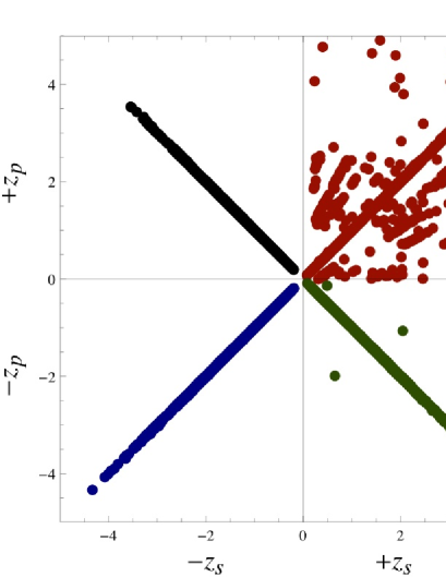
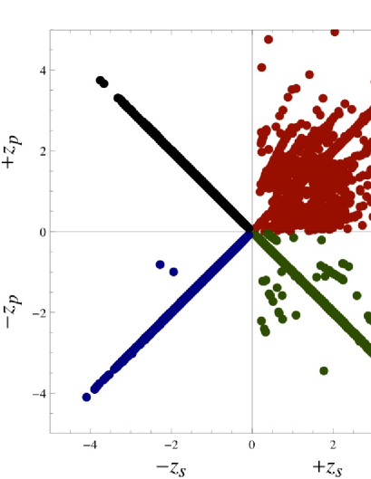
Figure 8: Scatter-plots of spectroscopic redshifts (horizontal axis) versus photometric redshifts (vertical axis) obtained with the template fitting method, for the four quality grade groups (1, 2, 3 and 4). Left panel: original sample; right panel: simulated sample. There are 2,500 objects in the group $g_{1}$ (first quadrant in the upper right corner, red dots in color version); 2,500 objects in the group $g_{2}$ (second quadrant and green dots); 2,500 objects in the group $g_{3}$ (third quadrant and blue dots); and 2,500 objects in the group $g_{4}$ (fourth quadrant and black dots). The radial lines in the $g_{1}$ group correspond to degenerate regions of the $z_{p}-z_{s}$ mapping. There are virtually no catastrophic errors for $z_{p}\gtrsim 2.5$ objects in the $g_{2}$, $g_{3}$ and $g_{4}$ grades in the simulated samples.

The median and median absolute deviation (mad) of the redshift errors in each grade groups are shown in Fig. 9, for the original (left panel) and simulated (right panel) samples. For the lowest quality photo-z’s (grade group 1), the median for the original sample of quasars is $med[|z_{p}-z_{s}|/(1+z_{s})]=0.0019$, and the deviation is $mad[|z_{p}-z_{s}|/(1+z_{s})]=0.0014$, which is very small given the high level of contamination from outliers – 12% for that group. For the simulated sample the redshift errors are much larger: the median and median deviation for group 1 are 0.0073 and 0.0069, respectively – which is not surprising given that the number of catastrophic photo-z’s is 44.7%. However, for the grade group 2 the median and median deviation for the original sample falls to 0.001 and 0.0007, respectively. More importantly, for the simulated sample the median and deviation are 0.0014 and 0.001, respectively. The accuracies of the photo-z’s for the grade groups 3 and 4 are slightly higher still.

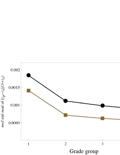
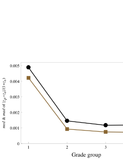
Figure 9: Median (med) and median absolute deviation (mad) of the errors in the photometric redshifts obtained with the template fitting method. Left panel: original sample of SDSS quasars; right panel: simulated sample. The circles (black in color version) denote the medians for each grade group; squares (brown in color version) denote the mad.

An alternative metric to assess the accuracy of the photometric redshifts is to manage the sensitivity to catastrophic outliers with the following method. First, we compute the tapered (or bounded) error estimator defined by:

$$\left(\frac{\sigma^{T}_{z}}{1+z}\right)^{2}=\left\langle\left[\delta_{z}\tanh\frac{1}{\delta_{z}}\frac{z_{p}-z_{s}}{1+z_{s}}\right]^{2}\right\rangle_{all}=$$ (8)

$$\frac{1}{N}\sum_{i}\left[\delta_{z}\tanh\frac{1}{\delta_{z}}\frac{z_{p}(i)-z_{s}(i)}{1+z_{s}(i)}\right]^{2}\;,$$

where $\delta_{z}=0.02$ in our case. For accurate quasar photo-z’s ($z_{p}\approx z_{s}$) with minimal contamination from outliers, this error estimator yields the usual contribution to the rms error, while for samples heavily influenced by catastrophic photo-z’s, this estimator assigns a contribution which asymptotes to our threshold $\delta_{z}.$

Second, we compute the purged rms error, summing only over the non-catastrophic photo-z’s:

$$\left(\frac{\sigma_{z}^{nc}}{1+z}\right)^{2}=\frac{1}{N^{nc}}\sum_{i=1}^{N^{nc}}\frac{[z_{p}(i)-z_{s}(i)]^{2}}{[1+z_{s}(i)]^{2}}\;.$$ (9)

The estimators (8)-(9) are therefore complementary: the tapered error estimator is indicative of the rate of catastrophic errors, while the purged rms error is a more faithful representation of the overall accuracy of the method for the bulk of the objects. The results for the two estimators of the photometric redshift uncertainties are shown in Fig. 10, for the four grade groups. The two estimators are in good agreement for the groups $g_{2}$, $g_{3}$ and $g_{4}$, which is again evidence that the rate of catastrophic photo-z’s is negligible for these groups.

Thus, we conclude that with the template fitting method alone it is possible to reach a photo-z accuracy better than $|z_{s}-z_{p}|/(1+z_{s})\sim 0.0015$ for at least $\sim 75\%$ of quasars, even for a population of faint objects (our simulated sample), with a very small rate of catastrophic redshift errors. In fact, the average accuracy given by the median and median deviation errors is already of the order of the intrinsic error in the spectroscopic redshifts due to line shifts [Shen et al. (2007, 2010)]. This means that, with filters of width $\sim$ 100 Å (or, equivalently, with low-resolution spectroscopy with $R\sim 50$) we are saturating the accuracy with which redshifts of quasars can be reliably estimated – although, naturally, with better resolution spectra and larger signal-to-noise the rate of catastrophic errors would be even smaller.

It is useful to compare the results of this section with those of the COMBO-17 quasar sample [Wolf et al. (2003b)]. That catalog, which employs five broad filters ($ugriz$) and 12 narrow-band filters, attains a photo-z accuracy of $\sigma_{z}=0.03$ – the same that was also obtained for the COMBO-17 galaxy catalog [Wolf et al. (2003a)]. The accuracy that we obtain for quasars with the 42 contiguous narrow-band filters is also of the same order as that which is obtained for red and emission-line galaxies [Benítez et al. (2009)]. Clearly, the gains in photo-z accuracy are not linear with the width of the filters, and the issue of continuous coverage over the entire dynamic range also plays in important role.

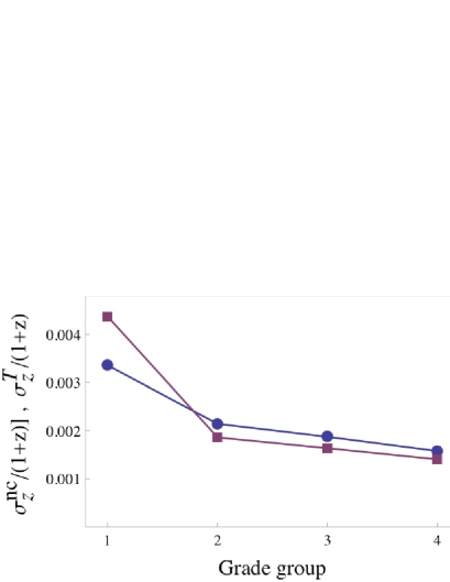
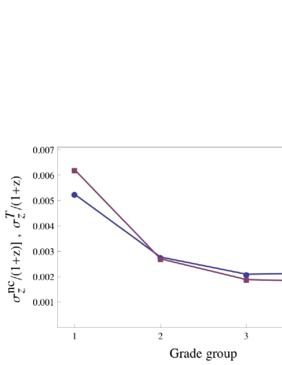
Figure 10: Photo-z errors obtained with the template fitting method for each grade group: (i) circles (blue in color version): rms error excluding catastrophic redshift errors, cf. Eq. 9; and (ii) squares (red in color version): rms tapered error including catastrophic redshift errors, cf. Eq. 8. When these two quantities coincide, the fraction of catastrophic photo-z’s has become negligible.

Finally, in order to understand how the photometric depth relates to photo-z depth, it is useful to compare the photo-z quality indicator for each object to the i-band magnitude of the simulated sample, $i_{s}$, as well as the dependence of the actual photo-z errors with $i_{s}$. The magnitude is directly related to the SNR through Eq. (2). From the left panel of Fig. 11 (which should also be compared to the right panel of Fig. 7) we see that the quality indicator declines steeply for the faintest objects in the simulated sample. From the right panel of Fig. 11 we see that the actual photo-z errors (which are plotted on an inverted scale) also depend on the magnitude, but in this case even for the faintest objects a substantial fraction of the quasars still have correctly estimated redshifts. This means that our quality indicator (which was calibrated for the full sample, independently of magnitude) is not very good at capturing the photo-z dependence for the faintest objects. Clearly, a more accurate analysis than the one we have implemented can be achieved by including the magnitudes as additional parameters for estimating the photo-z’s.

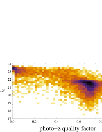
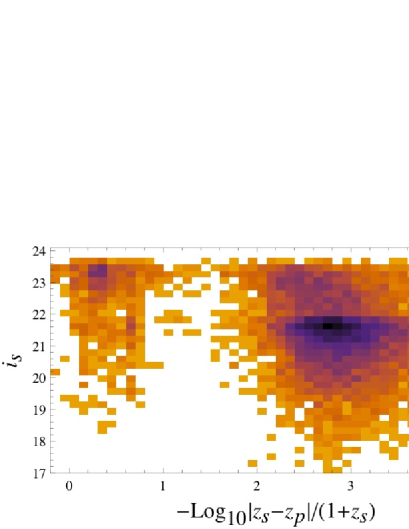
Figure 11: 2D histogram of the simulated sample, showing the magnitude in the $i$-band versus the photo-z quality indicator (left panel), and the magnitude versus the photo-z error on an inverted scale (right panel). These plots should be compared with the right panel of Fig. 7.

2.4 Photometric redshifts of quasars: Training Set Method

Training methods of redshift estimation are particularly well suited when a large and representative set of objects with known spectroscopic redshifts is available [Connolly et al. (1995); Firth et al. (2003); Csabai et al. (2003); Collister & Lahav (2004); Oyaizu et al. (2008); Banerji et al. (2008); Bonfield et al. (2010); Hildebrandt et al. (2010)]. Ideally this training set must be a fair sample of the photometric set of galaxies for which we want to estimate redshifts, reproducing its color and magnitude distributions. Whereas lack of coverage in certain regions of parameter space may imply significant degradation in photo-z quality, having a representative and dense training set can lead to a superior photo-z accuracy compared to template fits.

Empirical methods use the training set objects to determine a functional relationship between photometric observables (e.g. colors, magnitudes, types, etc.) and redshift. Once this function is calibrated, usually requiring that it reproduces the redshifts of the training set as well as possible, it can be straightforwardly applied to any photometric sample of interest. This class of methods includes machine learning techniques such as nearest neighbors [Csabai et al. (2003)], local polynomial fits [Connolly et al. (1995); Csabai et al. (2003); Oyaizu et al. (2008)], global neural networks [Firth et al. (2003); Collister & Lahav (2004); Oyaizu et al. (2008)], and gaussian processes [Bonfield et al. (2010)]. They have also been successfully applied to galaxy surveys, e.g. the SDSS [Oyaizu et al. (2008)], allowing further applications in cluster detection [Dong et al. (2008)] and weak lensing [Mandelbaum et al. (2008); Sheldon et al. (2009)].

The training set can also be used to improve template fitting, using it either to generate good priors or for empirical calibration and/or determination of the templates by, e.g., PCA of the spectra. Training sets are usually necessary to assess the photo-z quality of a certain survey specification and for calibration of the photo-z errors, which can then be modeled and included in a cosmological analysis [Ma et al. (2006); Lima & Hu (2007)]. In this sense, it is the knowledge of the photo-z error parameters – and not the value of the errors themselves – that limit the extraction of cosmological information from large data sets.

Here we implement a very simple empirical method, mainly to compare it with the template method presented in the previous Section. We use a simple nearest neighbor (NN) method: for each photometric quasar, we search the training set for its nearest neighbor in magnitude space, and then assign that neighbor’s spectroscopic redshift as the best estimate for the photo-z of the photometric quasar. We define distances with an Euclidean metric in multidimensional magnitude space, such that the distance $d_{ij}$ between objects $i$ and $j$ is:

$$d_{ij}^{2}=\sum_{a=1}^{N}(m^{a}_{i}-m^{a}_{j})^{2}\;,$$ (10)

where $N=42$ is the number of narrow filters and $m^{a}_{i}$ is the $a^{\rm th}$ magnitude of the $i^{\rm th}$ object. The nearest neighbor to a certain object $i$ is then simply the object $j$ for which $d_{ij}$ is minimum.

We computed photo-zs in this way for all $10^{4}$ quasars in the catalog. For each quasar, we took all others as the training set. In this case, there is no need to divide the objects into a training and photometric set, because all that matters is the nearest neighbor.

We can also use knowledge of the distance between the nearest neighbor and the second-nearest neighbor to assign a quality to the photo-z’s obtained with the training set method. The idea is that the quality of the photo-z is related to how sparse the training set is in the region around any given object. The original and simulated samples were then divided into four groups of increasing density (i.e., decreasing sparseness), as we did for the template fitting method. In Fig. 12 we show the photo-z’s as a function of spectroscopic redshifts for the original sample of quasars (left panel), and for the sample simulated with J-PAS specifications (right panel), for the four quality groups.

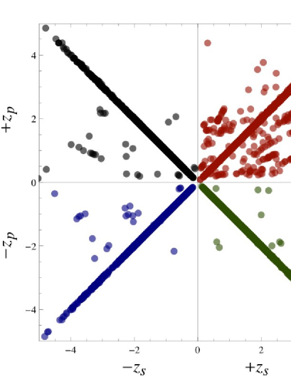
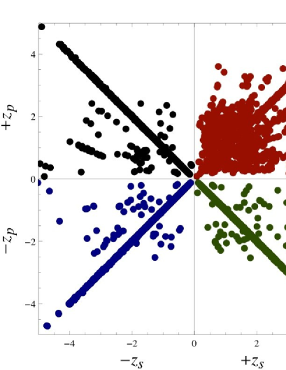
Figure 12: Scatter-plots of spectroscopic redshifts (horizontal axis) versus photometric redshifts (vertical axis) obtained with the training set method, for the four groups of decreasing sparseness (1, 2, 3 and 4, in decreasing sparseness). Left panel: original sample; right panel: simulated sample. As before, there are 2,500 objects in the first group (first quadrant in the upper right corner, red dots in color version); 2,500 objects in the second group (second quadrant and green dots); 2,500 objects in the third group (third quadrant and blue dots); and 2,500 objects in the fourth group (fourth quadrant and black dots).

The results for the median and median deviation of $|z_{s}-z_{p}|/(1+z_{s})$ are shown in Fig. 13. Although the fraction of outliers for groups 2-4 is roughly the same (at the level of 2-3%), the median and the median deviation of the photo-z errors are clearly correlated with the density of the training set. Comparing with Fig. 9 we see that the training set has a lower accuracy than the template fitting method – both the median and the median deviation of the training set groups are about twice as large as those of the template fitting groups.

The rms error after removing catastrophic objects with $\delta_{z}>0.02(1+z)$ is, for the original sample, $\sigma_{z}^{nc}/(1+z)=0.035$, 0.001, 0.0016 and 0.0037 for the sparseness bins 1-4. For the simulated sample the rms errors after eliminating the outliers are $\sigma_{z}^{nc}/(1+z)=0.082$, 0.0045, 0.0045 and 0.007 for the sparseness bins 1-4. For the photo-z groups 2, 3 and 4, the errors as measured by this criterium are about 2-3 times as large as the ones obtained with the template fitting method (see Fig. 10).

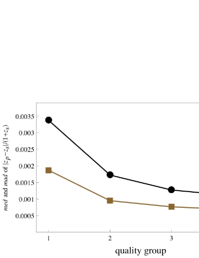
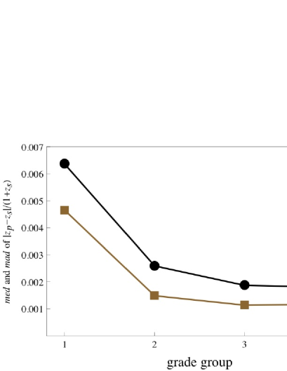
Figure 13: Median (med) and median absolute deviation (mad) of the errors in the photometric redshifts for the training set method. Left panel: original sample of SDSS quasars; right panel: simulated sample. The circles (black in color version) denote the medians for each grade group; squares (brown in color version) denote the mad.

We expect these results to improve significantly if we employ a denser training set. With the relatively sparse training set used here, we do not expect complex empirical methods to improve the photo-z accuracy. For instance, we have tried to use the set of the few nearest neighbors of a given object to fit a polynomial relation between magnitudes and redshifts, which we then applied to estimate the redshift of the photometric quasar. The results of such procedure were similar but slightly worse than simply taking the redshift of the nearest neighbor. That happens because our quasar sample is not dense enough to allow for stable global – and even local – fits.

With a sufficiently large training set, it has been shown that global neural network fits produce photo-z’s of similar accuracy to those obtained by local polynomial fits [Oyaizu et al. (2008)]. However these used a few hundred thousand training set galaxies spanning a redshift range of [0,0.3] whereas here we have $10^{4}$ quasars spanning the redshift range [0,5].

2.5 Comparison of the template fitting and training set methods

We have seen that the two methods for extracting the redshift of quasars, given a low-resolution spectrum, yield errors of the same order of magnitude. Both the template fitting (TF) and the training set (TS) methods also yield empirical criteria for selection of potential catastrophic redshift errors (the “quality factor" of the photo-z, in the case of the TF method, and the distance between nearest neighbors in the case of the TS method), which allows one to improve purity at the price of reducing completeness.

A larger sample of objects (the entire SDSS spectroscopic catalog of quasars, for instance, has $\sim 10^{5}$ objects, instead of the $\sim 10^{4}$ that we used in this work) would improve the performance of the TS method significantly, but may not necessarily make the performance of the TF method much better. A larger sample means a denser training set, which will certainly lead to better matches between nearby objects, as well as a better overall accuracy. From the perspective of the TF method, a larger sample only means a larger calibration set, and with our sample the performance of the method is already being driven not by the calibration, but by intrinsic spectral variations in quasars – something that the TS method is perhaps better suited to detect.

We have also applied a hybrid method to improve the quality of the photo-z’s even further, by combining the power of the TF and TS methods in such a way that one serves to calibrate the other. The method was implemented for the simulated sample of quasars in the following manner. First, we eliminate the 10% worst photo-z’s from the samples of quasars, either by using the quality factor, in the case of the TF method, or by using the distance between nearest neighbors, in the case of the TS method. This procedure alone reduces the median of the errors, $\Delta z/(1+z)$, to 0.0014 (TF) and 0.0024 (TS), and reduces the fraction of outliers to 5% (TF) and 4% (TS).

The next step is to flag as potential outliers all objects which have been rejected by either one of the 10% cuts, and to eliminate them from both samples – i.e., objects rejected by one method are also culled from the sample that survives the cut from the other method. The result is a culled sample containing about 83.6% of the initial $10^{4}$ objects. In that sample, the fraction of outliers is further reduced to 3.5% (TF) and 2.6% (TS).

The final step is to compare the two photo-z’s in the culled sets and flag those that differ by more than a certain threshold, namely $|z_{TF}-z_{TS}|/[1+0.5(z_{TF}+z_{TS})]=0.02$. After removing the flagged objects we still retain about 80% of the original sample (8001 quasars), but the fraction of outliers falls dramatically, to 0.6% (47 objects out of 8001). The median error for this final sample is 0.0013 (TF) and 0.0023 (TS), and the median deviation is 0.00084 (TF) and 0.0014 (TS).

Hence, the combination of the TF and TS methods can yield 80% completeness with 99.4% purity, and quasar photo-z errors which are as good as the spectroscopic ones. The histogram in Fig. 14 illustrates how this hybrid method is able to identify the outliers, and Table 1 shows how the performance of the photo-z estimation is enhanced by the successive cuts. Although the TS method is slightly better than the TF method at identifying the outliers, it is significantly worse in terms of the accuracy of the photo-z’s. However, the performance of the TS method should improve with a larger (and therefore denser) training set.

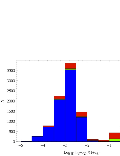
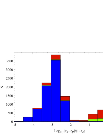
Figure 14: Histograms of the photo-z errors for the simulated sample of quasars. The left and right panels correspond to the template fitting (TF) and training set (TS) methods, respectively. The first quality cut (i.e., the quality factor in the case of the TF method, and the distance between nearest neighbors in the case of the TS method) reduces the full sample of $10^{4}$ quasars by 15% (upper bars, red in color version). The second cut, obtained by comparing the photo-z’s from each method, further reduces the number of quasars to 80% of the full sample (i.e., 8001 objects). The rate of outliers in this final sample is approximately 0.6% – see Table 1.

Table 1: Completeness (fraction of objects that remain after applying the cuts), purity (fraction of objects after culling the outliers) and accuracy of the photo-z’s for the simulated sample of quasars. The first step eliminates the 10% worst-quality photo-z’s in both techniques, producing the samples TF₉₀ and TS₉₀. The second step keeps only those objects which are present both in TF₉₀ and in TS₉₀, producing the samples TF_c and TS_c. The last step is to compare the photo-z’s that were obtained with the different techniques, and to flag those that differ by more than the threshold $\Delta z/(1+z)\geq 0.02$ as potential outliers.

Method	Completeness (%)	Purity (%)	$median\,[\,\Delta z/(1+z)\,]$
TF90 = TF - TF10	90	95	0.0014
TS90 = TS - TS10	90	96	0.0024
TFc = TF90 - TS10	85	96.5	0.0014
TSc = TS90 - TF10	86	97.4	0.0023
TFc v. TSc	80	99.4	0.0013
TSc v. TFc	80	99.4	0.0023

As a final note, there are a few important factors that we have not considered, which may affect the performance of the quasar photo-z’s. One of them is the calibration of the filters, which, if poorly determined, could introduce fluctuations of (typically) a few percent in the fluxes. Since J-PAS uses a secondary, 0.8 m aperture telescope dedicated to the calibration of the filter system, the stated goal of reaching 3% global homogeneous calibration seems feasible – and, in fact, we employed that lower limit for the noise level of our simulated quasar sample. An even more important factor is the time variability of the intrinsic SEDs of quasars, which can be a much larger effect than the fluctuations induced by calibration errors. Since a final decision concerning the strategy of the J-PAS survey has not yet been reached at the time this paper was finished, we decided not to pursue a simulation that took variability into account. However, it seems likely that each quasar that is observed by J-PAS will have several (7 or more) adjacent filters measured during an interval of a few (4-10) days, at most, and the full SED will be represented by a few (4-8) of these snapshots. In that sense, the information in the time domain contained by these snapshots would not be simply a nuisance, but may be used to aid in the identification of the quasars.

2.6 Completeness and contamination

In order to understand how a quasar sample produced from an optical narrow-band survey could be contaminated by other types of objects (stars, mostly), we have used data from SDSS spectroscopic plates in which a random subsample of all point sources with $i<19$ had their spectra taken [Adelman-McCarthy et al. (2006)]. We randomly extracted $10^{4}$ stars from this catalog, and processed their spectra using the template fitting method that was outlined in the previous subsections for the SDSS simulated quasars. However, we do not include any star templates in our fitting procedure, so the only questions we are asking are: (i) what is the redshift which best fits the quasar template spectrum to the spectra of each individual star, and (ii) what are the qualities of those fits (their reduced $\chi^{2}$)?

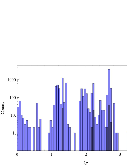
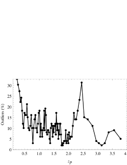
Figure 15: Left panel: photo-z’s assigned to stars by the quasar template fitting code, in 100 bins of redshift. The 1% stars with the highest potential to be confused with quasars (i.e., those whose spectra satisfy both $\chi^{2}<3.0$ and $r<0.75$) are shown as dark bars. Right panel: fraction of photo-z outliers [i.e., quasars whose photo-z’s differ from the correct redshifts by more than 0.02(1+z)] for the simulated quasar catalog, in 100 bins of redshift.

Using the tools which were introduced in Section 2.3 we were able to reject the overwhelming majority of stars, just on the basis of their poor reduced $\chi^{2}$ fits to the quasar template, and the degeneracy in their photo-z’s as measured by the parameter $r$ of Section 2.3 (stars lack the quasar’s emission-line features, which are the key determinants of the photo-z’s, and this translates into high values of $r$). Hence, it is clear that, in this sense, stars are quite segregated from quasars – and the introduction of stellar templates would further improve this separation. As a comparison, the COMBO-17 quasar catalog [Wolf et al. (2003b)] doesn’t suffer from significant contamination from stars, even though it has a lower spectral resolution than J-PAS, and similar depths. Hence, we conclude that the prospects of J-PAS achieving high levels of purity and completeness are quite good – however, we cannot definitively answer this question here, and leave this critical issue to future work.

Nevertheless, we can determine which redshift ranges are most likely to affect the completeness and purity of the quasar sample due to contamination from stars. Fig. 15 shows that the photo-z’s falsely assigned to stars are concentrated in a few intervals, corresponding to redshifts where the visible region of the quasar spectra present few distinguishing features. The concentration of false photo-z’s in narrow intervals is starker for those stars whose spectra can most easily be confused with those of quasars – which, for the purposes of this exercise, are stars whose fits to the quasar template satisfy both $\chi^{2}<3$ and $r<0.75$ (approximately 1% of the total). Some of these problematic redshift intervals also contain a large proportion of the catastrophic photo-z’s for the true quasars (see the right panel of Fig. 15). These plots indicate that contamination should be a greater concern for the redshift intervals $1.30\lesssim z_{p}\lesssim 1.31$, $2.2\lesssim z_{p}\lesssim 2.22$ and $2.65\lesssim z_{p}\lesssim 2.7$.

3 Quasars as cosmological probes

The SDSS sample of quasars [Richards et al. (2001); Vanden Berk et al. (2001); Schneider et al. (2003); Yip et al. (2004); Schneider et al. (2007); Shen et al. (2007); Ross et al. (2009); Schneider et al. (2010); Shen et al. (2010)] has enabled a reliable measurement of the quasar luminosity function [Richards et al. (2005, 2006); Hopkins et al. (2007); Croom et al. (2009a, b)], which, in terms of the g-band absolute magnitude is given by the fit [Croom et al. (2009b)]:

$$\phi(M_{G},z)=\frac{\phi_{0}}{10^{0.4\,(1+\alpha)\,[M_{G}-M_{G}^{*}(z)]}+10^{0.4\,(1+\beta)\,[M_{G}-M_{G}^{*}(z)]}}\;,$$ (11)

where $\phi_{0}=1.57\times 10^{-6}$ Mpc^-3, $\alpha=-3.33$, $\beta=-1.41$ and the break magnitude expressed in terms of $M_{G}$ is given by:

$$M_{G}^{*}(z)=-22.2-2.5\,(1.44\,z-0.32\,z^{2})\;.$$ (12)

Notice that the quasar luminosity function and the break magnitude were obtained with a sample of quasars only up to $z\sim 2.5$, and it is far from clear that these fits can be extrapolated to higher redshifts and lower luminosities [Croom et al. (2009b)].

To obtain the number density of quasars as a function of some limiting (absolute) magnitude $M_{G}^{0}$, the luminosity function above must be integrated up to that magnitude. In Fig. 16 we plot the quasar volumetric density both in terms of the limiting apparent magnitude in the $g$ band for flux-limited surveys, $n(<g_{lim})=\int_{-\infty}^{g_{\lim}}dg\ \phi(g)$ (solid lines, $g_{\lim}=$ 24, 23, 21 and 19, from top to bottom), and also in terms of the absolute magnitudes $n(<M_{G,\lim})=\int_{-\infty}^{M_{G,\lim}}dM_{G}\ \phi(M_{G})$ (dashed lines, $M_{G,\lim}=$ -20, -22, -24 and -26 from top to bottom.) Since contamination from the host galaxy may hinder our ability to identify low-luminosity quasars through color selection (this can be especially problematic at low redshifts), we chose to apply a cut in absolute magnitude in the luminosity function, in addition to the apparent magnitude cut.

As a concrete example, we will discuss a flux-limited survey up to an apparent magnitude of $g<23$, and include only those objects which are more luminous than $M_{G}<-22$, since quasars fainter than this often have their light dominated by the host galaxy. The resulting comoving number density is shown as the dashed line and hashed region in Fig. 16, which peaks at $z\sim 1.6$ with $n_{\rm max}\sim 10^{-5}$ Mpc^-3 (or $\sim 3.10^{-4}\,h^{3}$ Mpc^-3.) If the limiting apparent magnitude is $g<24$, the number density can be as large as $10^{-4}\,h^{3}$ Mpc^-3 at $z\sim 2$. As we will see below, the relatively small density of quasars when compared to galaxies (which can easily reach $n\gtrsim 10^{-3}$ Mpc^-3) is compensated by the facts that quasars are highly biased tracers of large-scale structure, and that the volume that they span is larger than that which can be achieved with galaxies – for a similar analysis, see also Wang et al. (2009); Sawangwit et al. (2011).

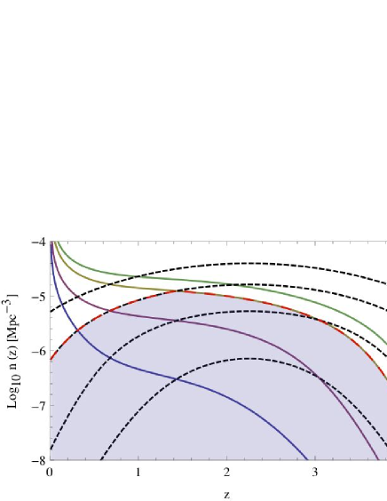
Figure 16: The volumetric density of quasars for different limiting $g$-band apparent magnitudes (solid lines) and different absolute magnitudes (dashed lines), as a function of redshift, computed according to the luminosity function of Croom et al. 2009. The solid lines, from top to bottom, correspond to limiting magnitudes of $g\leq$ 24 (green in color version), 23 (yellow in color version), 21 (red in color version) and 19 (blue in color version); the short-dashed lines, from top to bottom, correspond to absolute luminosity cut-offs of $M_{G}\leq$ -20, -22, -24 and -26 respectively.

It is also useful to compute the total number of quasars that a large-area (1/5 of the sky), flux-limited survey could produce – assuming the quasar selection is perfect. In Fig. 17 we show that an $8.4\times 10^{3}$ deg² survey up to $g<23$ ($g<24$) could yield $2.0\times 10^{6}$ ($3.0\times 10^{6}$) objects, up to $z=5$.

Figure 17: Total numbers of quasars in $\Delta z=0.5$ bins for an $8.4\times 10^{3}$ deg² survey, assuming a $5\sigma$ point-source magnitude limit of $g=$ 23 (left bars, red in color version) and 24 (right bars, blue in color version.) The numbers are identical for $z\leq 1.5$ because our selection criteria culls the quasars fainter than $M_{G}=-22$, which means that for $z<1.5$ the catalog is equivalent to a volume-limited and absolute magnitude-limited survey.

3.1 Large-scale structure with quasars

Quasars, like any other type of extragalactic sources, are biased tracers of the underlying mass distribution: $P_{q}(k,z)=b_{q}^{2}(z)P(k,z)$, where $P(k,z)$ is the matter power spectrum, $P_{q}(k,z)$ is quasar power spectrum (the Fourier transform of the quasar two-point correlation function), and $b_{q}$ is the quasar bias. The quasar bias is a steep function of redshift [Shen et al. (2007); Ross et al. (2009)], and it may depend weakly on the intrinsic (absolute) luminosities of the quasars [Lidz et al. (2006)], but it is thought to be independent of scale ($k$) – at least on large scales.

The connection between theory and observations is further complicated by the fact that both the observed two-point correlation function and the power spectrum inherit an anisotropic component due to redshift-space distortions [Hamilton (1997)]. In this work we will only consider the monopole of the power spectrum, $P(k)=\int_{-1}^{1}d\mu P(k,\mu)$, where $\mu$ is the cosine of the angle between the tangential and the radial modes. We will address the full redshift-space dataset from our putative quasar survey, as well as the resulting constraints thereof, in future work.

To first approximation the statistical uncertainty in the power spectrum can be estimated using the formula derived in Feldman et al. (1994) for three-dimensional surveys:

$$\frac{\Delta P(k,z)}{P(k,z)}\simeq\sqrt{\frac{2}{N_{m}(k,z)}}\left[1+\frac{1}{n(z)b^{2}(z)P(k,z)}\right]\;,$$ (13)

where $n$ is the average number density of the objects used to trace large-scale structure, and $b$ is the bias of that tracer. The number of modes (the statistically independent degrees of freedom) in a given bin in $k$-space is given by $N_{m}=4\pi V(z,z+\Delta z)k^{2}\Delta k/(2\pi)^{3}$, where $\Delta z$ and $\Delta k$ denote the thickness of the redshift bins and of the wavenumber bins, respectively. The first term inside the brackets in Eq. 13 corresponds to sample variance, and the second corresponds to shot noise (assuming the variance of the shot noise term is that of a Poisson distribution of the counts.) Since the power spectrum peaks at $P\lesssim 10^{4.5}\,h^{-3}$ Mpc³, a quasar survey with $n\lesssim 10^{-5}\,h^{3}$ Mpc^-3 would be almost always limited by shot noise.

For the purposes of this exercise we have used 28 bins in Fourier space, equally spaced in $\log(k)$, and spanning the interval between $0.007$ $h$ Mpc${}^{-1}<k<1.4$ $h$ Mpc^-1. Our reference matter power spectrum $P_{0}(k,z)$ is a modified BBKS spectrum [Bardeen et al. (1986)] [see also Peacock (1999) or Amendola & Tsujikawa (2010)]. The transfer function of the BBKS fit does not contain the BAO modulations, so we have modeled those features in the spectrum by means of the fit [Seo & Eisenstein (2007); see also Benítez et al. (2009)]:

$$P(k,z)=P_{0}(k,z)\left[1+kA\sin(kr_{BAO})e^{-k^{2}R^{2}}\right]\;,$$ (14)

where $r_{BAO}=146.8$ Mpc = $105.7\,h^{-1}$ Mpc is the length scale of the BAOs that can be inferred from WMAP [Hinshaw et al. (2009)], $A=0.017\,r_{BAO}$ is the amplitude of the acoustic oscillations, and $R=10\,h^{-1}$ Mpc denotes the Silk damping scale.

Eq. (13) is an approximation which is appropriate for spectroscopic redshift surveys, although this is not the type of survey that we are considering. Nevertheless, we have showed in the previous Section that, with narrow-band filters, the error in the photo-z’s of quasars can be lower than $\delta z\sim 0.002\,(1+z)$, which is excellent but not quite equivalent to a spectroscopic redshift. Redshift errors smear structures on small scales along the line-of-sight, and can be factored into the estimation of the power spectrum through an empirical damping term [Angulo et al. (2008)]:

$$\exp{\left[-k_{\parallel}^{2}\frac{\delta_{z}^{2}c^{2}}{H^{2}(z)}\right]}\;,$$ (15)

where $k_{\parallel}=k\mu$ denote the modes along the line-of-sight. In our $\Lambda$CDM model, photometric redshift errors suppress modes which are smaller than about $k_{\parallel}^{-1}\,\sim\,\delta_{z}\times 10^{3}h^{-1}$ Mpc at $z=2$ (or $k_{\parallel}^{-1}\,\sim\,\delta_{z}\times 5.10^{2}h^{-1}$ Mpc at $z=4$). Hence, a quasar photo-z error of the order of $0.002(1+z)$ only starts to affect the power spectrum at scales $k_{\parallel}\gtrsim 0.2h$ Mpc^-1 at z=2, and $k_{\parallel}\gtrsim 0.4h$ Mpc^-1 at z=4. This is smaller than either the Silk damping scale or the scales at which nonlinear effects kick in (see the discussion below), so we expect that photo-z errors will be a subdominant nuisance in the estimation of the power spectrum and derived parameter constraints.

Another important point concerning Eq. (13) is that it applies to the power spectrum as estimated by some biased tracer, but it does not automatically include the uncertainty in the bias or the selection function, or other systematic effects such as bias stochasticity [Dekel & Lahav (1999)]. Here we employ the fit found by [Ross et al. (2009)] for quasars with $z<2.2$, which is given by $b_{q}(z)=0.53+0.29\,(1+z)^{2}$. Although this bias has large uncertainties, especially at high redshifts, we will implicitly assume that $b_{q}(z)$ is a linear, deterministic bias that has been fixed at each redshift by this fit.

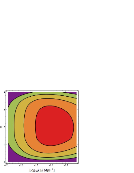
Figure 18: The contours denote the statistical errors in the power spectrum, $\log_{10}\Delta P(k,z)/P(k,z)$, for an $8.4\times 10^{3}$ deg² quasar survey, flux-limited down to $g<23$, and limited to objects brighter than $M_{G}=-22$. From inside to outside, the contours correspond to $\Delta P/P=10^{-1.5}$, $10^{-1}$, $10^{-0.5}$ and $10^{0}$. The uncertainties were computed using Eq. 13. For this plot we binned the redshift slices in intervals of $\Delta z=0.1$, and the wavenumbers were divided into 28 equally spaced bins in $\log(k)$, spanning the interval between $k=0.007\,h$ Mpc^-1 and $k=1.4\,h$ Mpc^-1. Photo-z errors and uncertainties in the bias of quasars are not included in our error budget.

In Fig. 18 we plot the contours corresponding to equal uncertainties in the power spectrum as a function of the scale [$\log_{10}k$ (h Mpc^-1), horizontal axis)] and redshift $z$ (vertical axis), according to Eqs. (11)-(14), and assuming that the J-PAS survey covers $8.4\times 10^{3}$ deg² to a $5\sigma$ limiting magnitude of $g<23$. There are three main effects that determine the shape of the contours in Fig. 18: first, at fixed $k$ and low redshifts, both the volume of the survey as well as the number density of objects (which is determined by the absolute luminosity cut) are small, while at high redshifts the number density falls rapidly due to the apparent magnitude cut. Second, for a fixed $z$ the uncertainty as a function of $k$ decreases up to scales $k\sim 0.02\,h$ Mpc^-1, where $P(k)$ peaks, and as it starts to fall, it increases the Poisson noise term in Eq. (13). Finally, the redshift evolution of the power spectrum [$P(k,z)\sim D^{2}(z)$, where $D(z)$ is the linear growth function] also increases the shot noise at higher redshifts – although this effect is partly mitigated by the redshift evolution of the quasar bias. Quasars achieve their best performance in estimating the power spectrum at $z\sim$ 1 – 3. This is because in that range the quasar bias increases faster than the number density falls as a function of redshift.

A closely related way of assessing the potential of a survey to measure the power spectrum is through the so-called effective volume:

$$V_{\rm eff}(k)=\int d^{3}x\left[\frac{n\,b^{2}\,P(k)}{1+n\,b^{2}\,P(k)}\right]^{2}\,,$$

where $x$ is comoving distance, and both the average number density $n$ and the bias $b$ are presumably only functions of $x$ (or, equivalently, of redshift). The effective volume is simply (twice) the Fisher matrix element that corresponds to the optimal (bias-weighted) estimator of the power spectrum [Feldman et al. (1994); Tegmark et al. (1998)]. In Fig. 19 we show the effective volume for our quasar survey (full line). For comparison, we have also plotted the effective volume of a hypothetical quasar survey similar to BOSS or BigBOSS, that would target $\sim 5.10^{5}$ objects over the same area and with the same redshift distribution as the J-PAS quasar survey (long-dashed line). Also plotted in Fig. 19 are the effective volumes of two surveys of LRGs assuming the luminosity function of Brown et al. (2007), either in the case of a shallow survey flux-limited to $g<21.5$ (“SDSS-like”, short-dashed line), or for a deep survey limited to $i<23$ (“J-PAS-like”, dashed line.)

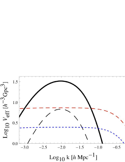
Figure 19: Effective volume of a flux-limited quasar catalog ($g<23$ and $z<4$) over $8.4\times 10^{3}$ deg². We also show the effective volume of a putative spectroscopic survey of quasars with $4.10^{5}$ objects, where we assumed the same area and redshift distribution as was used for the J-PAS catalog (“BOSS-like", long-dashed line.) For comparison, we also show two hypothetical catalogs of luminous red galaxies (LRGs) over the same area, one limited to $g<21.5$ (“SDSS-like”, short-dashed line, blue in color version) and the other limited to $i<23$ (long-dashed line, red in color version.) For the LRG estimates, we used the luminosity function of Brown et al. (2007) and assumed a constant bias $b_{\rm LRG}=1.5$.

In Fig. 20 we plot the power spectrum divided by the BBKS power spectrum $P_{0}(k)$, in order to highlight the BAO features. The error bars, from leftmost to rightmost (black in color version to orange in color version), corresponds to measurements of the power spectrum in redshit bins of $\Delta z=0.5$ centered in $z=0.5$, $z=1.0$, $z=1.5$, $z=2.0$, $z=2.5$ and $z=3.0$, respectively. The power spectrum at low redshifts is poorly constrained, but this improves at high redshifts ($z\sim 1-3$).

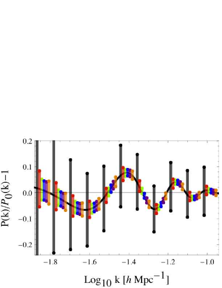
Figure 20: Baryon acoustic oscillations in position space. The oscillations are highlighted by dividing the full spectrum by a reference BBKS spectrum $P_{0}(k)$ without the baryon acoustic features. From left to right, the error bars correspond to the uncertainties at $z=0.5$ (black curve and grey error bars), $z=1.0$ (red), $z=1.5$ (green), $z=2.0$ (blue), $z=2.5$ (purple), and $z=3.0$ (orange). In this plot we employed redshift bins of $\Delta z=0.5$. The errors of the $z=0.5$ bin are much larger than those of other bins because: i) the volume of the $z=0.5$ bin is much smaller than that of other bins, which makes cosmic variance worse; and ii) the quasar luminosity function is more dominated by faint objects at low redshifts (see Fig. 16), and since we have culled those objects with our absolute luminosity cut, $M_{G}<-22$, the volumetric density drops by a large factor, thus increasing shot noise.

Figs. 18-20 demonstrate that quasars are not only viable tracers of large-scale structure, but they can also detect the BAO features at high redshifts. An interesting advantage of a high-redshift measurement of BAOs is the milder influence of redshift distortions and nonlinear effects. In linear perturbation theory, the redshift-space and the real-space spectra are related by $P^{(s)}_{q}/P^{(r)}_{q}\simeq 1+\frac{2}{3}\beta_{q}+\frac{1}{5}\beta_{q}^{2}$ [Kaiser (1987); Hamilton (1997)], where $\beta_{q}\simeq\Omega_{m}^{0.55}/b_{q}$ in a flat $\Lambda$CDM Universe. Redshift distortions in the nonlinear regime are more difficult to take into account, but they also scale roughly with $\beta_{q}$ – see, e.g., Jain & Bertschinger (1994); Meiksin et al. (2001); Scoccimarro et al. (2010); Seo et al. (2010); Smith et al. (2006); Angulo et al. (2008); Seo et al. (2008). Since quasars become more highly biased at high redshifts, both linear and nonlinear redshift-space distortions are suppressed relative to the local Universe.

The effect of random motions can be taken into accounted by multiplying the redshift-space spectrum factor of $1/[1+k^{2}\sigma_{s}(z)^{2}]$, where $\sigma_{s}(z)$ is a smoothing scale related to the one-dimensional pairwise velocity dispersion, and is usually calibrated by numerical simulations. Nonlinear growth of structure and bulk flows (which tend to smear out the BAO signature) also decrease at higher redshifts [Smith et al. (2006); Seo et al. (2008)]. Angulo et al. (2008) found a useful parametrization of this effect in terms of a Fourier-space smoothing kernel $W(k,k_{nl})=\exp[-k^{2}/2k_{nl}^{2}]$, where $k_{nl}(z)$ is a non-linear scale determined by numerical simulations.

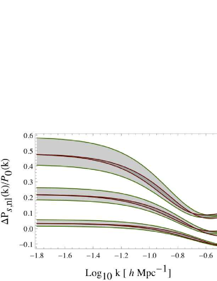
Figure 21: Scaling of the redshift distortions (outer, lighter contours and green lines in color version) and of the effects of nonlinear structure formation (inner, darker contours and red lines in color version), for $z=1$, $z=2$ and $z=3$ from top to bottom, respectively. The uncertainties caused by redshift distortions and nonlinear effects, $\Delta_{s,nl}P/P_{0}$, are indicated by the hashed regions. For visual clarity, we shifted the distortions at $z=1$ by $+0.1$, and the distortions at $z=3$ by $-0.1$. We use the empirical calibration and errors of Angulo et al. 2008 for the redshift and nonlinear distortions. For the quasar bias and its uncertainties we employ the fit of Ross et al. (2009).

In Fig. 21 we plot both the redshift distortions in linear theory, and the nonlinear effects on the power spectrum. For the redshift distortions we employ the quasar bias obtained in Ross et al. (2009):

$$b_{q}=(0.53\pm 0.19)+(0.289\pm 0.035)(1+z)^{2}\;,$$

which we assume holds up to $z=3$ (even though the uncertainties are very large at such high redshifts.) For the smoothing parameter we have extrapolated the data from Angulo et al. (2008), and found $\sigma_{s}\simeq(4-0.96z)h^{-1}$ Mpc (this approximation is good up to $z\simeq 3$.)

Finally, nonlinear structure formation effects are taken into account by the nonlinear scale given in Angulo et al. (2008) (which are appropriate for halos heavier than $M>5\times 10^{13}M_{\odot}$):

$$k_{nl}(z)=(0.096\pm 0.0074)+(0.036\pm 0.0094)z\;,$$

in units of $h$ Mpc^-1.

With these assumptions, the ratio between the non-linear power spectrum in redshift space and the linear, position-space power spectrum is modeled by:

$$\frac{P^{(s,nl)}_{q}(k,z)}{P^{(r,l)}_{q}(k,z)}=1+\left(\frac{1+\frac{2}{3}\beta+\frac{1}{5}\beta^{2}}{1+k^{2}\sigma^{2}}-1\right)\,e^{-k^{2}/2k_{nl}^{2}}\;.$$

Fig. 21 illustrates that the distortions become smaller at higher redshifts, and that the uncertainties associated with them are also being suppressed.

In conclusion, we have seen that a large-area catalog of quasars, down to depths of approximately $g<23$, can yield a precision measurement of the power spectrum and of BAOs at moderate and high redshifts. The fact that quasars can measure large-scale structure even better than LRGs around the peak of the power spectrum, despite their much smaller volumetric density, can be understood as follows. First, the volume spanned by quasars is larger, since they are much more luminous and can be seen to higher redshifts than galaxies. This makes both sample variance and shot noise smaller by a factor of the square root of the volume, according to Eq. (13). Second, although the number density of quasars is at least one order of magnitude smaller than that of LRGs, the bias of quasars increases rapidly with redshift, and becomes higher than that of LRGs at $z\sim 1$. Since the volumetric factor which determines shot noise is the product of the number density and the square of the bias, ($nb^{2}$), a highly biased tracer such as quasars can afford to have a relatively small number density. At or near the peak of the power spectrum, the accuracy of the power spectrum of quasars is almost limited by sample variance; slightly away from the peak, shot noise becomes increasingly relevant, but the vast volume occupied by a catalog of quasars means that they are still superior compared to red galaxies. It is only on very small scales, where the amplitude of the power spectrum is very small, that galaxies become superior to quasars by virtue of their much higher number densities – but then again, this only works at the relatively low redshifts where galaxies can be efficiently observed.

How, then, could such a catalog of quasars be constructed? One possibility is multi-object spectroscopy. While target selection of quasars from broad-band photometry can be quite efficient in certain redshift ranges [such as z<2.2 for the SDSS filter set [Richards et al. (2001)], there are ranges of redshifts where the broad-band optical colors of quasars and the much more numerous stars are indistinguishable, especially in the presence of photometric errors. There is the additional problem of contamination from galaxies, but this should be a subdominant effect compared to stars (we leave this issue for future work). The comoving space density of quasars peaks between z=2.5 and 3, just the redshift at which the color locus of quasars crosses the stellar locus [Fan (1999)], and selecting quasars in this redshift range tends to be quite inefficient and difficult [Richards et al. (2008); Ross et al. (2011)].

A more concrete possibility is a narrow-band photometric survey, such as J-PAS, which will take low-resolution spectra of all objects (including quasars) in the surveyed area. However, there are two problems with this technique: first, unless the photometric redshifts of the quasars are very accurate, the relative errors in their radial positions could be so large as to destroy their potential to map large-scale structure. This is even more critical if we want to measure the signature of BAOs in the angular and radial directions. In the previous Section we showed that it is possible to obtain very small photo-z errors, so this should not be the main concern. The main problem will be the classification of point sources as either quasars or stars, especially for low-luminosity objects whose fluxes are noisy. Although stars and quasars can be distinguished by criteria such as the $\chi^{2}$ of their fits to templates, as well as the level of degeneracy of the PDF’s of their photo-z’s, stars vastly outnumber quasars, and hence stringent criteria must be used in order to preserve the purity of the quasar sample. This may compromise the completeness (and therefore the final number density) of the quasar catalog, which would then lead to large levels of shot noise.

Hence, the key to realizing the potential of quasars to measure large-scale structure in a narrow-band photometric survey hinges on whether or not we can type a sufficiently high proportion of quasars, and obtain accurate photometric redshifts for the majority of objects in that catalog. In the previous section we showed that this may be possible with an instrument such as J-PAS. However, our results can be easily generalized to other surveys such as Alhambra (which goes deeper than J-PAS, but has broader filters) and HETDEX (which subtends a smaller area and has a similar depth compared with J-PAS, but has much better spectral resolution).

4 Conclusions

We have argued that quasars are viable tracers of large-scale structure in the Universe. A wide and deep survey of these objects will be a zero-cost consequence of several ongoing or planned galaxy surveys that use either narrow-band filter systems or integral field low-resolution spectroscopy.

Our estimates indicate that a dataset containing millions of objects will be a sub-product of these spectrophotometric surveys, and that they can lead not only to measurements of the distribution of matter in the Universe up to very high redshifts ($z\lesssim 4$), but also to an improved understanding of these objects, how they evolved, what are their clustering properties and bias, as well as their relationship and co-evolution with the host galaxies. Such a large dataset, spread over such vast volumes, will also allow a range of applications that break these objects into sub-groups (of absolute magnitude, types of host galaxies, etc.)

We have also shown that with a narrow-band set of filters (of width $\sim$ 100 Å in the optical) it is possible to obtain near-spectroscopic photometric redshifts for quasars: $\sigma_{z}\sim 0.001(1+z)$ with the template fitting method, and at least $\sigma_{z}\sim 0.002(1+z)$ with the training set method. This means an unprecedented resolution along the direction of the line-of-sight that extends up to vast distances, and is a further reason for using quasars as tracers of large-scale structure.

References

- Abbott et al. (2005) Abbott T. et al., 2005, astro-ph/0510346
- Abdalla et al. (2008a) Abdalla F., Banerji M., Lahav O., Rashkov V., 2008, arXiv e-print 0812.3831
- Abdalla et al. (2008b) Abdalla F., Amara A., Capak P., Cypriano E., Lahav O., Rhodes J., 2008, MNRAS , 387, 969
- Abdalla et al. (2008c) Abdalla F., Mateus A., Santos W., Sodrè L., Ferreras I., Lahav O., 2008, MNRAS , 387, 945
- Abell (2009) Abell P. et al., 2009, 0912.0201
- Adelman-McCarthy et al. (2006) Adelman-McCarthy J. K. et al., 2006, ApJS, 162, 38
- Adelman-McCarthy et al. (2008a) Adelman-McCarthy J. K. et al. 2008, VizieR Online Data Catalog, 2282, 0
- Adelman-McCarthy et al. (2008b) Adelman-McCarthy J. K. et al., 2008, ApJS, 175, 297
- Amendola & Tsujikawa (2010) Amendola L., Tsujikawa S., 2010, Dark Energy: Theory and Observations. Cambridge University Press
- Angulo et al. (2008) Angulo R., Baugh C. M., Frenk C. S., Lacey C. G., 2007, MNRAS , 383, 755
- Baldwin (1977) Baldwin J. A., 1977, ApJ, 214, 679
- Banerji et al. (2008) Banerji, M. and Abdalla, F. B. and Lahav, O. and Lin, H., 2008, MNRAS , 386, 1219
- Bardeen et al. (1986) Bardeen J. M., Bond J. R., Kaiser N., Szalay A. S., 1986, The ApJ, 304, 15
- Baum (1962) Baum W. A., 1962, in IAUS Vol. 15, Photoelectric magnitudes and Red-Shifts. p. 390
- Benítez (2000) Benítez N., 2000, ApJ, 536, 571
- Benítez et al. (2009) Benítez N. et al., 2009, ApJ, 691, 241
- Blake & Glazebrook (2003) Blake, C., Glazebrook, K., 2003, ApJ, 594, 665
- Blake & Bridle (2005) Blake C., Bridle S., 2005, MNRAS , 363, 1329
- Blake et al. (2007) Blake C., Collister A., Bridle S., Lahav O., 2007, MNRAS, 374, 1527
- Bolzonella et al. (2000) Bolzonella M., Miralles J., Pelló R., 2000, A&A, 363, 476
- Bond & Efstathiou (1984) Bond, J. R., Efstathiou, G., 1984, ApJ, 285, L45
- Bonfield et al. (2010) Bonfield D. G., Sun Y., Davey N., Jarvis M. J., Abdalla F. B., Banerji M., Adams R. G., 2010, MNRAS , 405, 987
- Brown et al. (2007) Brown M. J. I., Dey A., Jannuzi B. T., Brand K., Benson A. J., Brodwin M., Croton D. J., Eisenhardt P. R., 2007, ApJ, 654, 858
- Bruzual & Charlot (2003) Bruzual G., Charlot S., 2003, MNRAS , 344, 1000
- Budavári (2009) Budavári T., 2009, ApJ, 695, 747
- Coil et al. (2010) Coil A. L. et al., 2010, ArXiv e-prints 1011.4307
- Cole et al. (2005) Cole S. et al., 2005, MNRAS , 362, 505
- Collister & Lahav (2004) Collister, A. A. and Lahav, O., 2004, PASP, 116, 345
- Connolly et al. (1995) Connolly A. J., Csabai I., Szalay A. S., Koo D. C., Kron R. G., Munn J. A., 1995, AJ, 110, 2655
- Cool (2008) Cool R. J., 2008, PhD thesis, The University of Arizona
- Croft et al. (1998) Croft R. A. C., Weinberg D. H., Katz N., Hernquist L., 1998, ApJ, 495, 44
- Croom et al. (2004) Croom S. M., Smith R. J., Boyle B. J., Shanks T., Miller L., Outram P. J., Loaring N. S., 2004, MNRAS , 349, 1397
- Croom et al. (2005) Croom S. M., Boyle B. J., Shanks T., Smith R. J., Miller L., Outram P. J., Loaring N. S., Hoyle F., da Ângela J., 2005, MNRAS , 356, 415
- Croom et al. (2009a) Croom S. M. et al., 2009, MNRAS , 392, 19
- Croom et al. (2009b) Croom S. M. et al., 2009, MNRAS , 399, 1755
- Csabai et al. (2003) Csabai I. et al., 2003, AJ, 125, 580
- da Ângela et al. (2005) da Ângela J. et al., 2005, MNRAS , 360, 1040
- Dekel & Lahav (1999) Dekel A., Lahav O., 1999, ApJ, 520, 24
- Dong et al. (2008) Dong F., Pierpaoli E., Gunn J. E., Wechsler R. H., 2008, ApJ, 676, 868
- Eisenstein & Hu (1999) Eisenstein D. J., Hu W., 1999, ApJ, 511, 5
- Eisenstein (2003) Eisenstein D. J., 2003, ApJ, 586, 718
- Eisenstein et al. (2005) Eisenstein D. J. et al., 2005, ApJ, 633, 560
- Fan (1999) Fan X., 1999, AJ, 117, 2528
- Feldman et al. (1994) Feldman H. A., Kaiser N., Peacock J. A., 1994, ApJ, 426, 23
- Firth et al. (2003) Firth A. E., Lahav O., Somerville R. S., 2003, MNRAS , 339, 1195
- Hamilton (1997) Hamilton A. J. S., 1997, in “The Evolving Universe”, ed. D. Hamilton, Kluwer Academic, p. 185 (1998), arXiv e-print astro-ph/9708102
- Hildebrandt et al. (2010) Hildebrandt, H. et al., 2010, A&A, 523, A31
- Hinshaw et al. (2009) Hinshaw G., et al., 2009, ApJS, 180, 225
- Holtzman (1989) Holtzman J., 1989, ApJS, 71, 1
- Hopkins et al. (2007) Hopkins P. F., Richards G. T., Hernquist L., 2007, ApJ, 654, 731
- Hu & Sugiyama (1995) Hu W. & Sugiyama N., 1996, ApJ, 471, 542
- Jain & Bertschinger (1994) Jain B., Bertschinger E., 1994, ApJ, 431, 495
- Kaiser (1987) Kaiser N., 1987, MNRAS , 227, 1
- Kormendy & Richstone (1995) Kormendy J., Richstone D., 1995, Ann. Rev. Astron. Astroph., 33, 581
- Lidz et al. (2006) Lidz A., Hopkins P. F., Cox T. J., Hernquist L., Robertson B., 2006, ApJ, 641, 41
- Lima & Hu (2007) Lima, M., Hu, W., Phys. Rev. D76, 123013
- Lynden-Bell (1969) Lynden-Bell D., 1969, Nature, 223, 690
- Ma et al. (2006) Ma Z., Hu W., Huterer D., 2006, ApJ, 636, 21
- Mandelbaum et al. (2008) Mandelbaum R. et al., 2008, MNRAS , 386, 781
- Martini & Weinberg (2001) Martini P., Weinberg D. H., 2001, ApJ, 547, 12
- Meiksin et al. (2001) Meiksin A., White M., Peacock J. A., 1999, MNRAS , 304, 851
- Moles et al. (2008) Moles M. et al., 2008, AJ, 136, 1325
- Moles et al. (2010) Moles M. et al., 2010, PASP, 122, 363
- Oyaizu et al. (2008) Oyaizu H., Lima M., Cunha C. E., Lin H., Frieman J., Sheldon E. S., 2008, ApJ, 674, 768
- Padmanabhan et al. (2005) Padmanabhan N. et al., 2005, MNRAS , 359, 237
- Padmanabhan et al. (2007) Padmanabhan N. et al., 2007, MNRAS , 378, 852
- Padmanabhan et al. (2008) Padmanabhan N., White M., Norberg P., Porciani C., 2008, MNRAS , 397, 1862
- Peacock (1999) Peacock J. A., 1999, Cosmological Physics. New York: Cambridge University Press
- Peebles & Yu (1970) Peebles P. J. E., Yu J. T., 1970, ApJ, 162, 815
- Percival et al. (2007) Percival W. J. et al., 2007, MNRAS , 381, 1053
- Porciani et al. (2004) Porciani C., Magliocchetti M., Norberg P., 2004, MNRAS, 355, 1010
- Richards et al. (2005) Richards G. T. et al., 2005, MNRAS , 360, 839
- Richards et al. (2002) Richards G. T. et al., 2002, AJ, 123, 2945
- Richards et al. (2008) Richards G. T. et al., 2008, ApJS, 180, 67
- Richards et al. (2006) Richards G. T. et al., 2006, AJ, 131, 2766
- Richards et al. (2001) Richards G. T. et al., 2001, AJ, 122, 1151
- Richstone et al. (1998) Richstone D. et al., 1998, Nature, 395, 14
- Ross et al. (2011) Ross N. P. et al., 2011, ArXiv e-prints 1105.0606
- Ross et al. (2009) Ross N. P. et al., 2009, ApJ, 697, 1634
- Salpeter (1964) Salpeter E. E., 1964, ApJ, 140, 796
- Salvato et al. (2009) Salvato M. et al., 2009, ApJ, 690, 1250
- Sawangwit et al. (2011) Sawangwit U., Shanks T., Croom S. M., Drinkwater M. J., Fine S., Parkinson D., Ross N. P., 2011, ArXiv e-prints 1108.1198
- Schlegel et al. (1998) Schlegel D. J., Finkbeiner D. P., Davis M., 1998, ApJ, 500, 525
- Schneider et al. (2003) Schneider D. P. et al., 2003, AJ, 126, 2579
- Schneider et al. (2007) Schneider D. P. et al., 2003, AJ, 134, 102
- Schneider et al. (2010) Schneider D. P. et al., 2010, AJ, 139, 23
- Scoccimarro et al. (2010) Scoccimarro R., Zaldarriaga M., Hui L., 1999, ApJ, 527, 1
- Scoville et al. (2007) Scoville N. et al., 2007, ApJS, 172, 1
- Seljak et al. (2005) Seljak U. et al., 2005, Phys. Rev. D71, 103515
- Seo & Eisenstein (2003) Seo H. J., Eisenstein D. J., 2003, ApJ, 598, 720
- Seo & Eisenstein (2007) Seo H.-J., Eisenstein D. J., 2007, ApJ, 665, 14
- Seo et al. (2008) Seo H. J., Siegel E. R., Eisenstein D. J., White M., 2008, ApJ, 686, 13
- Seo et al. (2010) Seo H. J., Eckel J., Eisenstein D. J., Mehta K., Metchnik M., Padmanabhan N. Pinto P., Takahashi R., White M., Xu X., 2010, ApJ, 720, 1650
- Sheldon et al. (2009) Sheldon, E. S. et al., 2009, ApJ, 703, 2217
- Shen et al. (2010) Shen Y. et al., 2010, ApJS, 194, 45
- Shen et al. (2007) Shen Y. et al., 2007, AJ, 133, 2222
- Smith et al. (2006) Smith R. E., Scoccimarro R., Sheth R. K., 2006, Phys. Rev. D75, 063512
- Sunyaev & Zeldovich (1970) Sunyaev R. A., Zeldovich Y. B., 1970, Astroph. Space Sc., 7, 20
- Tegmark et al. (2006) Tegmark M. et al., 2006, Phys. Rev. D74, 123507
- Tegmark et al. (1998) Tegmark M., Hamilton A. J. S., Strauss M. A., Vogeley M. S., Szalay A. S., 1998, ApJ, 499, 555
- Vanden Berk et al. (2001) Vanden Berk D. E. et al., 2001, AJ, 122, 549
- Wang et al. (2009) Wang X. et al., 2009, MNRAS , 394, 1775
- Wolf et al. (2003a) Wolf C. et al., 2003, A&A, 401, 73
- Wolf et al. (2003b) Wolf C. et al., 2003, A&A, 408, 499
- Yahata et al. (2005) Yahata K. et al., 2005, PASJ, 57, 529
- Yip et al. (2004) Yip C. W. et al., 2004, AJ, 128, 2603
- York et al. (2000) York D. G., et al., 2000, AJ, 120, 1579
- Zel’Dovich & Novikov (1965) Zel’Dovich Y. B., Novikov I. D., 1965, Soviet Physics Doklady, 9, 834