XMM-Newton observations of the dwarf nova RU Peg in quiescence: Probe of the boundary layer

Abstract

We present an analysis of X-ray and UV data obtained with the XMM-Newton Observatory of the long period dwarf nova RU Peg. RU Peg contains a massive white dwarf, possibly the hottest white dwarf in a dwarf nova, it has a low inclination, thus optimally exposing its X-ray emitting boundary layer, and has an excellent trigonometric parallax distance.

We modeled the X-ray data using XSPEC assuming a multi-temperature plasma emission model built from the MEKAL code (i.e., CEVMKL). We obtained a maximum temperature of 31.7 keV, based on the EPIC MOS1, 2 and pn data, indicating that RU Peg has an X-ray spectrum harder than most dwarf novae, except U Gem. This result is consistent with and indirectly confirms the large mass of the white dwarf in RU Peg. The X-ray luminosity we computed corresponds to a boundary layer luminosity for a mass accretion rate of $2\times 10^{-11}M_{\odot}$/yr (assuming $M_{wd}=1.3M_{\odot}$), in agreement with the expected quiescent accretion rate. The modeling of the O viii emission line at 19Å  as observed by the RGS implies a projected stellar rotational velocity $v_{rot}\sin{i}=$695 km s^-1, i.e. the line is emitted from material rotating at $\sim$936-1245 km s^-1 ($i\sim 34^{\circ}-48^{\circ}$) or about 1/6 of the Keplerian speed; this velocity is much larger than the rotation speed of the white dwarf inferred from the Far Ultraviolet Spectroscopic Explorer (FUSE) spectrum. Cross-correletion analysis yielded an undelayed (time lag $\sim$ 0) component and a delayed component of 116$\pm$17 sec where the X-ray variations/fluctuations lagged the UV variations. This indicates that the UV fluctuations in the inner disk are propagated into the X-ray emitting region in about 116 sec. The undelayed component may be related to irradiation effects.

1 Introduction

1.1 The long period dwarf nova RU Peg

Dwarf novae (DNe) are a class of weakly-magnetic cataclysmic variables (CVs) which are interacting compact binaries in which a white dwarf (WD, the primary star) accretes matter and angular momentum from a main (or post-main) sequence star (the secondary) filling its Roche-lobe. The matter is transferred, at a continuous or sporadic accretion rate ($\dot{M}$), by means of an accretion disk usually reaching all the way to the WD surface. Ongoing accretion at a low rate (quiescence) is interrupted every few weeks to months by intense accretion (outburst) of days to weeks (a dwarf nova accretion event). DNe are powerful X-ray sources with luminosities of $10^{30}-10^{33}$erg s^-1. The X-ray emission is believed to originate in the boundary layer (BL) between the slowly rotating accreting WD and the fast rotating (Keplerian) inner edge of the accretion disk, where the material dissipates its remaining rotational kinetic energy before it accretes onto the surface of the WD. The typical DNe, i.e. those systems exhibiting normal DN outbursts are the U Gem sub-type of DNe (according to the classification of Ritter & Kolb (2003)) and are located above the period gap ($P_{orb}>3$hr).

RU Peg is a U Gem type DN with an orbital period $P_{orb}$ = 8.99 hrs, a secondary spectral type K2-5V, a primary (WD) mass $M_{wd}=1.29_{-0.20}^{+0.16}M_{\odot}$, and a secondary mass $M_{2}=0.94\pm 0.04M_{\odot}$ (Stover, 1981; Wade, 1982; Shafter, 1983). The system has a magnitude range $V_{max}-V_{min}\approx 9.0-13.1$ with outbursts lasting $\sim$20 days and recurring every $\sim$50 days. The near-Chandrasekhar WD mass has been corroborated by the sodium (8190Å) doublet radial velocity study of Friend et al. (1990). They obtained a mass of 1.38$\pm$0.06 M_⊙ for the WD and also found a range of inclination angles between 34^∘-48^∘ in agreement with the range of plausible inclinations found in the study by Stover (1981). More recently, a Hubble Fine Guidance Sensor (FGS) parallax of $3.55\pm 0.26$ mas was measured by Johnson et al. (2003) yielding a distance of $282\pm 20$ pc.

RU Peg was observed with IUE under several different observing programs both in quiescence and in outburst and was part of several survey-like studies (e.g. La Dous et al. (1985); Verbunt (1987); Szkody et al. (1991) to cite just a few).

Sion & Urban (2002) modeled 4 IUE spectra obtained in deep quiescence with accretion disks and photospheres. They found that a very hot WD dominated the FUV spectrum with a temperature T${}_{eff}=50-53,000$K which places RU Peg among the hottest WDs in DNe. The distance corresponding to their best fitting, high gravity ($Log(g)=8.7$) photosphere models was 250 pc.

More recently, (Godon et al., 2008) modeled the FUSE spectrum of RU Peg in quiescence and obtained a WD with a temperature of 70,000K, a rotational velocity of 40 km s^-1, assuming $Log(g)=8.8$ and a distance of 282 pc. In this later study the higher temperature obtained in the model fitting is mainly a consequence of the assumed larger distance and gravity. It is clear that RU Peg has a massive WD and therefore a deep potential well, and its surface temperature is very large ($>$50,000K), possibly pointing to strong accretional and boundary layer heating. For these reasons, we chose RU Peg as our X-ray target, as it is expected to be a copious source of X-rays and should be an ideal candidate to study its boundary layer.

1.2 The Boundary Layer

The boundary layer is that region between the slowly rotating accreting WD and the fast rotating (Keplerian) inner edge of the accretion disk. For accretion to occur, gravity has to overcome the centrifugal acceleration, and this happens in the boundary layer as the material dissipates its remaining rotational kinetic energy before being accreted onto the surface of the WD. In the boundary layer the rotational velocity is sub-Keplerian and decreases inwards.

The standard disk theory (Shakura & Sunyaev, 1973) predicts a BL luminosity almost equal to the disk luminosity (Pringle, 1981) :

$$L_{BL}=(1-\beta^{2})L_{disk}=(1-\beta^{2})\frac{GM_{*}\dot{M}}{2R_{*}},$$ (1)

where $G$ is the gravitational constant, $M_{*}$ is the mass of the accreting star, $R_{*}$ its radius, $\dot{M}$ is the mass accretion rate, and $\beta$ is the stellar angular velocity in Keplerian units $\beta=\Omega_{*}/\Omega_{K}(R_{*})$. For most systems the WD rotational velocity is of the order of a few $100$ km s^-1 and one therefore has $\beta<<1$ and $L_{BL}\approx L_{disk}$. For a star rotating at (e.g.) 10% of the breakup velocity eq.(1) gives $L_{BL}=0.99L_{disk}$. However, the standard disk theory does not take into account the boundary layer explicitly. Using a one-dimensional approach, Kluźniak (1987) has shown that part of the BL (kinetic) energy actually goes into the spinning of the star in the equatorial region, and the BL luminosity is more accurately given by the relation

$$L_{BL}=\left(1-\beta\right)^{2}L_{disk}.$$ (2)

For a star rotating at 10% of the breakup velocity, eq.(2) gives $L_{BL}=0.81L_{disk}$, which is significantly different than eq.(1).

Because of its small radial extent, the BL is expected to emit its energy in the X-ray bands ($L_{BL}\approx L_{X-ray}$). At high accretion rate (or during dwarf nova outburst), the BL is expected to be optically thick with a temperature $T\approx 10^{5}-10^{6}$K (Godon et al., 1995; Popham & Narayan, 1995), and emits in the soft X-ray band. Observations of CVs in high state (e.g. Mauche et al. (1995); Baskill et al. (2005)) confirm these predictions. Accretion onto white dwarfs in some symbiotics presents similar soft X-ray emissions (Luna & Sokoloski, 2007; Luna et al., 2008; Kennea et al., 2009) because of the large mass accretion rates in these systems. At low mass accretion rate (or during dwarf nova quiescence), as the density is much decreased, the BL becomes optically thin and emits in the hard X-ray band with $T\approx 10^{8}$K (Narayan & Popham, 1993) (see below for observational evidence of such optically thin BLs). Hence, during quiescence the emission should arise from a very hot plasma very close to the WD surface.

Previous X-ray observations of dwarf nova systems in quiescence (e.g. van der Woerd & Heise (1987); van Teeseling & Verbunt (1996); Belloni et al. (1991)) while confirming the presence of hard X-ray, deduced that, contrary to the theory, the quiescent BL luminosity was underluminous. Namely, they found $L_{BL}=L_{X-ray}<<L_{disk}$, which confirmed the original claim that BLs were actually missing (Ferland et al. 1982). However, these earlier results assumed the disk to be the source of the optical and ultraviolet radiation ($L_{disk}=L_{opt}+L_{UV}$) and used eq.(1) rather than eq.(2). More recently, X-ray Multi Mirror-Newton (XMM-Newton) observations of 8 DNe in quiescence by Pandel et al. (2003, 2005) revealed that a significant part of the emitted FUV flux ($L_{UV}$) actually originates from the WD itself, and the evidence for underluminous BLs in quiescent DNe was refuted. For RU Peg, FUSE observations (Godon et al., 2008) indicate that the WD contributes possibly most of the FUV light with a temperature $T>50,000$K. In addition, Godon & Sion (2005) noted that the region where the boundary layer meets the inner edge of the Keplerian disk (Popham, 1999) can also contribute some FUV flux. It is clear now that one cannot just compare the X-ray luminosity to the optical + UV luminosity to check whether the boundary luminosity is as large as the disk luminosity.

For the 8 dwarf novae caught in quiescence, Pandel et al. (2003, 2005), using the XMM-Newton data, obtained X-ray boundary layer luminosities of the order of $\sim 1\times 10^{31}$ergs s^-1 to $6.6\times 10^{32}$ergs s^-1, with temperatures ranging from $\sim 8$ to $55$ keV, and mass accretion rates deduced from X-rays in the range $10^{-12}M_{\odot}$/yr to $10^{-10}M_{\odot}$/yr. In this work, we present XMM-Newton observations of RU Peg taken in quiescence to derive its X-ray luminosity and gain information on its boundary layer.

2 Observations and Analysis

The XMM-Newton Observatory (Jansen et al., 2001) has three 1500 cm² X-ray telescopes each with an European Photon Imaging Camera (EPIC) at the focus. Two of the telescopes have Multi-Object Spectrometer (MOS) CCDs (Turner et al., 2001) and the last one uses pn CCDs (Strüder et al., 2001) for data recording. There are two Reflection Grating Spectrometers (RGS) (den Herder et al., 2001). The Optical Monitor (OM), a photon counting instrument, is a co-aligned 30-cm optical/UV telescope, providing for the first time the possibility to observe simultaneously in the X-ray and optical/UV regime from a single platform (Mason et al., 2001).

RU Peg was observed (pointed observation) with XMM-Newton for an duration of 53.1 ks on June 9th, 2008, at 07:16:50.0 UTC (obsID 0551920101). At that time the system was at a visual magnitude of $\sim 12.5$, about 2 months into quiescence and 2 weeks before the next outburst (from AAVSO data ). Data were collected with the EPIC MOS and pn cameras in the prime partial window2 and prime full window imaging mode, respectively, the Reflection Grating Spectrometer and the Optical Monitor using the fast imaging mode ($\leq$0.5 sec time resolution) with the UVW1 filter (240-340 nm).

We analysed the pipeline-processed data using Science Analysis Software (SAS) version 9.0.0. Data (single- and double-pixel events, i.e., patterns 0–4 with Flag=0 option for pn and patterns $\leq$ 12 with Flag=0 for MOS1,2) were extracted from a circular region of radius 60^′′ for pn, and 45^′′ MOS1 & MOS2 in order to perform spectral analysis together with the background events extracted from a source free zone normalized to the source extraction area. We checked the pipeline-processed event file for any existing flaring episodes and no sporadic events in the background were detected with count rate higher than 0.08 c s^-1 (for MOS1,2) and 0.5 for pn detectors. Table 1 displays the background subtracted count rates for the EPIC pn, MOS1 and MOS2.

The RGS observations were carried out using the standard spectroscopy mode for readout. We reprocessed the data using the XMM-SAS routine rgsproc. We first made event files and determined times of low background from the count rate on CCD 9 (which is closest to the optical axis). The final exposure times and net count rates showed that there were no sporadic high background events in our data. Table 1 displays the background subtracted count rates for RGS1 and RGS2. Source and background counts for the RGS were extracted using the standard spatial and energy filters for the source position, which defines the spatial extraction regions as well as the wavelength zero point.

2.1 X-ray and UV Light curves

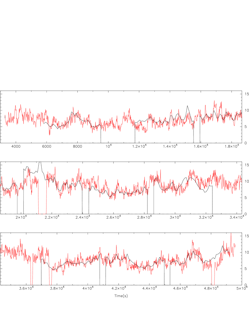
Figure 1: The EPIC X-ray light curve (binned at 16 s, in red) together with the OM UV light curve (binned here at 100 s for display, in black; the data were binned at 20 s for the correlation check). The count rate of the UV data has been divided by 9.1736 to fit the count rate level of the X-ray data for easier comparison. The time $t=0$ corresponds to $t=3.29389320\times 10^{8}$s, counted from the MJD reference day 50,814, namely: 54,626.376 MJD. The time modulation of the UV data follows closely the time modulation of the X-ray data except around $t\approx$12 ks, 20-22 ks, 31 ks, & 48.5 ks, where the UV has relatively more flux.

The UV and EPIC pn X-ray light curves are shown together for comparison in Figure 1, where we have scaled the UV count rate to fit the X-ray count rate for a better comparison. The count rate for the UV data ranges between $\sim$50 c/s and $\sim$100 c/s with a time average of $\sim$71.8 c/s. For UV-bright objects, a count rate of 1 s^-1 in the UVW1 filter translates into a flux of $4.5\times 10^{-16}$ergs cm^-2s^-1Å^-1 at 290 nm (see the online XMM-Newton documentation). This gives for RU Peg a flux of $\approx 2.2-4.5\times 10^{-14}$ergs cm^-2s^-1Å^-1, corresponding to a luminosity of $\approx 2.1-4.3\times 10^{29}$ergs s^-1Å ^-1 (at a distance d=282pc). The time modulation of the UV data follows closely the time modulation of the X-ray data except around $t\approx$12 ks, 20-22 ks, 31 ks, & 48.5 ks, where the UV has relatively more flux for a duration of several hundred seconds (and up to 1,000 s). Since the UV is expected to be emitted further out than the X-rays, these four epochs where the UV light curves do not decrease as much as the X-rays might be due to the occultation of the X-ray emitting material by the WD, while the UV emitting region is not hidden from the observer.

In order to study the correlation between the X-ray and the UV variability, we calculated the cross-correlation between the two light curves. We used time bins of 5 sec averaging several power spectra with 128 bins for the analysis. The resulting correlation coefficient as a function of time lag is shown in Figures 2a & 2b. The correlation coefficient is normalized to have a maximum value of 1. The curve shows a clear asymmetry indicating existence of time delays. We, also, detect a strong peak near zero time lag suggesting a significant correlation between X-rays and the UV light curves. We call this the undelayed component (see Figures 2a & 2b). The positive time-lag in the asymmetric profile shows that the X-ray variations are delayed relative to those in the UV. In order to calculate an average time-lag that would produce the asymmetric profile, we fitted the varying cross-correlation by two lorentzians, with time parameter fixed at 0.0 lag and the other set as free. The resulting fit yields a lag of 116$\pm$17 sec. This is the delayed component.

2.2 EPIC Spectrum

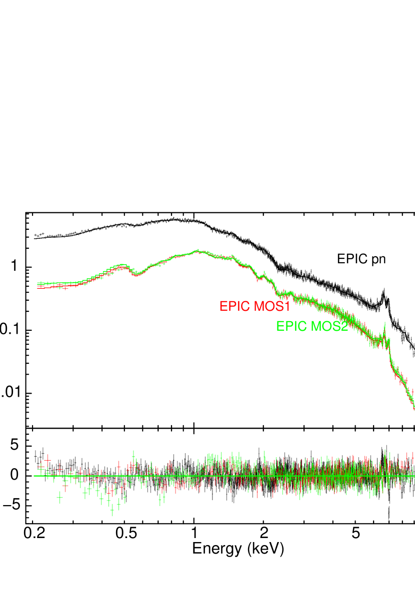
Figure 3: EPIC MOS1,2 and pn spectra simultaneously fitted to the same model TBabs$\times$CEVMKL. The model includes an ISM absorption model and a multi-temperature plasma emission model built from the MEKAL code. The maximum shock temperature obtained from the fit is 31.7 keV. The second panel below the fitted spectra is the residuals in standard deviations. One can notice a slight CTI problem of the pn detector around the iron lines (6.4-6.9 keV) where the fluctuations in the residuals due to CTI are evident. This does not affect the global fitting procedure but only slightly increases the reduced $\chi^{2}$ of the fits.

We performed spectral analysis of the EPIC data using the SAS task ESPECGET and derived the spectra of the source and the background together with the appropriate response matrices and ancillary files. How the photons were extracted is described in Section 2. The EPIC pn, EPIC MOS1 and EPIC MOS2 spectra were simultaneously fitted to derive the spectral parameters. The spectral analysis was performed using XSPEC version 12.6.0q (Arnaud 1996). A constant factor was included in the spectral fitting to allow for a normalization uncertainty between the EPIC pn and EPIC MOS instruments. We grouped the pn and MOS spectral energy channels so that there is a minimum of 80 (MOS1,2)-150 (pn) counts in a bin to improve the statistical quality of the spectra. The fits were conducted in the 0.2-10.0 keV range. The simultaneously fitted spectra from the three EPIC instruments are shown in Figure 3. We modeled the X-ray spectrum of RU Peg in a similar fashion as Pandel et al. (2005) and fitted the data with (TBabs$\times$CEVMKL) model within XSPEC. TBabs is the Tuebingen-Boulder ISM absorption model (Wilms, Allen and McCray 2000) and CEVMKL is a multi-temperature plasma emission model built from the mekal code (Mewe et al., 1985). Emission measures follow a power-law in temperature (i.e. emission measure from temperature T is proportional to $(T/T_{max})^{\alpha-1}$). The residuals in Figure 3 show systematic fluctuation around the 6.7-6.9 keV iron line complex mainly from the EPIC pn data and some small low energy fluctuations exist in the MOS2 data, as well. This is due to the CTI (Charge transfer inefficiency) problem, in the pn (and possibly MOS2) instrument. These generally occur around lines due to small calibration errors and mostly effect only the line shapes leaving systematic residuals and increasing the reduced $\chi^{2}$ of the fits. Our EPIC MOS1 data does not exhibit any CTI effects and the reduced $\chi^{2}$ for the fit to this data alone is 1.15 (d.o.f. 290). The reduced $\chi^{2}$ for the simultaneously fitted spectra is higher than the value for the MOS1 fit, but the spectral parameters for all three instruments are almost the same within the errors. Table 2 contains the spectral parameters from fits (using three detectors simultaneously) with the (TBabs$\times$CEVMKL) model. Errors are given at 90% conf. level. We find a maximum plasma temperature in a range 29-33 keV and mostly solar abundances of elements aside from oxygen and neon which we calculate to be subsolar. The unabsorbed X-ray flux is 4.1${}^{+0.2}_{-0.2}$$\times 10^{-11}$ erg s^-1cm^-2 which translates to a luminosity of 4.1${}^{+0.3}_{-0.3}$$\times 10^{32}$ erg s^-1 at 282 pc (see sec. 1). The neutral hydrogen column density is 4.3-4.5$\times 10^{20}$ cm^-2.

2.3 RGS Spectrum

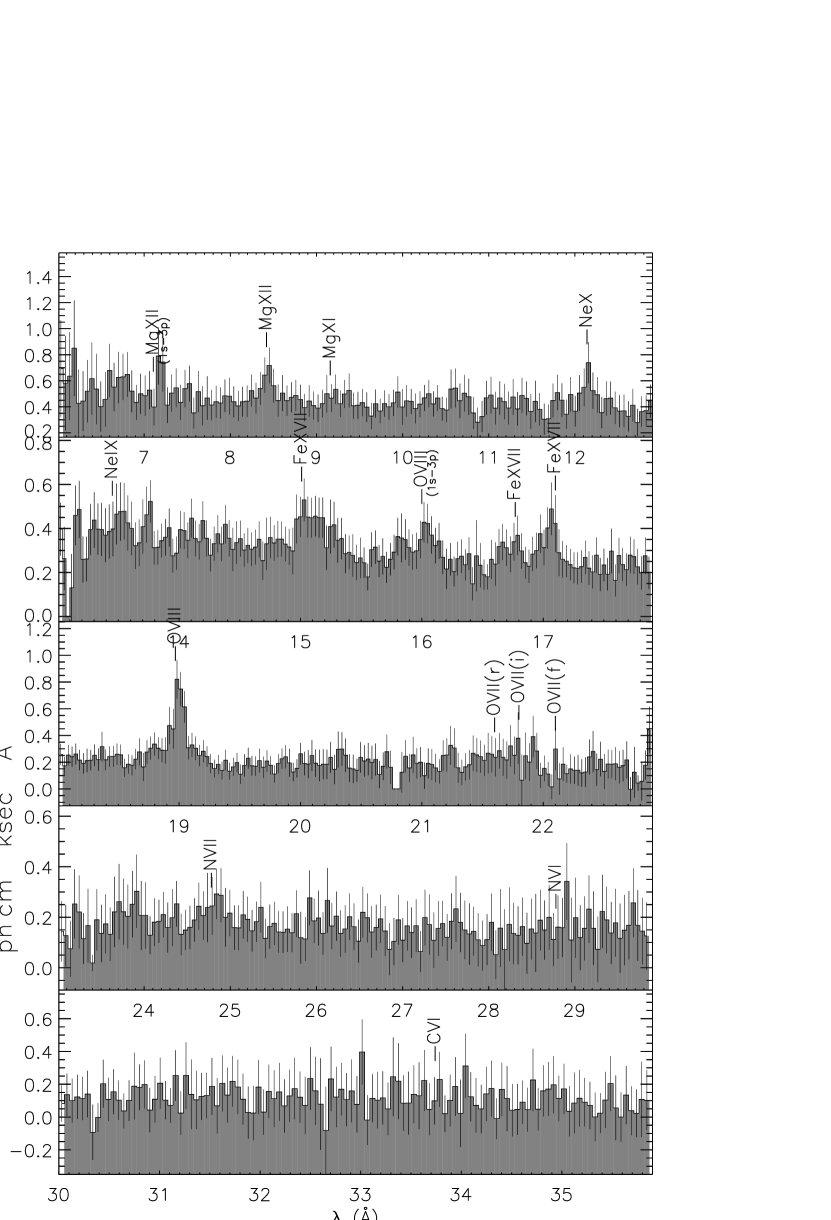
Figure 4: The fluxed RGS Spectrum of RU Peg with line identifications.

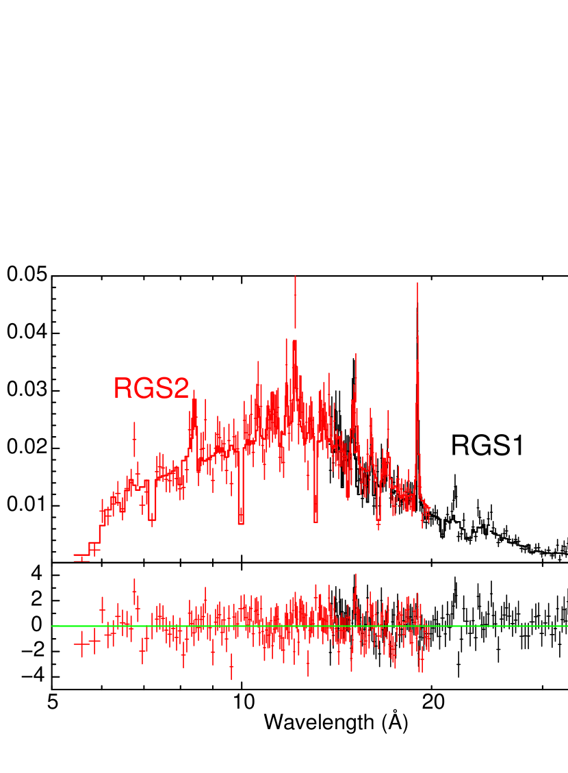
Figure 5: The simultaneously fitted RGS 1 and RGS 2 spectrum of RU Peg. The same model TBabs$\times$CEVMKL is used for the fit. The residuals in the second panel below are in standard deviations.

The RGS analysis tool rgsproc was used to obtain RGS1 and RGS2 spectra and to produce fluxed spectrum (i.e., using rgsfluxer) The resultant fluxed spectrum of the combined RGS1 and RGS2 detectors is shown in Figure 4 with line identifications. The detected lines and corresponding wavelengths are listed in Table 3. Fluxed spectra are obtained just by dividing the count spectrum by the RGS effective area. It neglects the redistribution of monochromatic response into the dispersion channels. Since proper response is not utilized by the fluxed spectrum, in order to perform a similar spectral fit/analysis using the same (TBabs$\times$CEVMKL) model within XSPEC, we used the count rate spectra produced for RGS1 and RGS2 simultaneously with the appropriate response files for each detector. This is a very efficient approach to find the spectral parameters in comparison with the EPIC results. The fitted RGS1 and RGS2 spectra are shown in Figure 5. Table 4 contains the spectral parameters from the fit with the (TBabs$\times$CEVMKL) model within XSPEC. Errors are 90% conf. level and the fit is performed between 0.2-2.5 keV.

The maximum temperature from the fits with the RGS data yield 24 keV with a large error range of 17-41 keV since the spectrum has a lower count rate and a lower upper energy boundary (i.e., 2.5 keV) compared with the EPIC data (i.e., 12 keV). We find that most of the RGS spectral parameters are consistent for the EPIC results. Oxygen and neon are subsolar in abundance and silicon appears to be slightly enhanced compared to solar abundance. The resolution of the RGS spectra is sufficient to measure the rotational velocity of the bounday layer via Doppler broadening of emission lines. We calculated the broadening using the O viii emission line at 19Å which is the strongest line in the spectrum. We used a Gaussian model to calculate the $\sigma$ of the line ($\sigma\times 2.4$=FWHM) along with a power-law/bremmstrahlung for the continuum. We find that FWHM=0.044Å and the corresponding velocity in the line of sight is 695 km s^-1 ($\Delta\lambda$/$\lambda$ = $v/c$). We also checked the resolution of RGS at around 19Å and found 0.04-0.05 Å and we caution that our measurement is on the limit of the RGS spectral resolution.

3 Discussion

The maximum X-ray shock temperature we obtain is 29-33 keV, based on the EPIC MOS1, 2 and pn data, as they have higher count rates and braoder energy ranges than the RGS data. RU Peg has a harder X-ray spectrum than in most dwarf novae, but softer than U Gem in quiescence, which also contains a massive white dwarf (Sion et al., 1998; Long & Gilliland, 1999). This result is consistent with and confirms the large mass of the white dwarf in RU Peg.

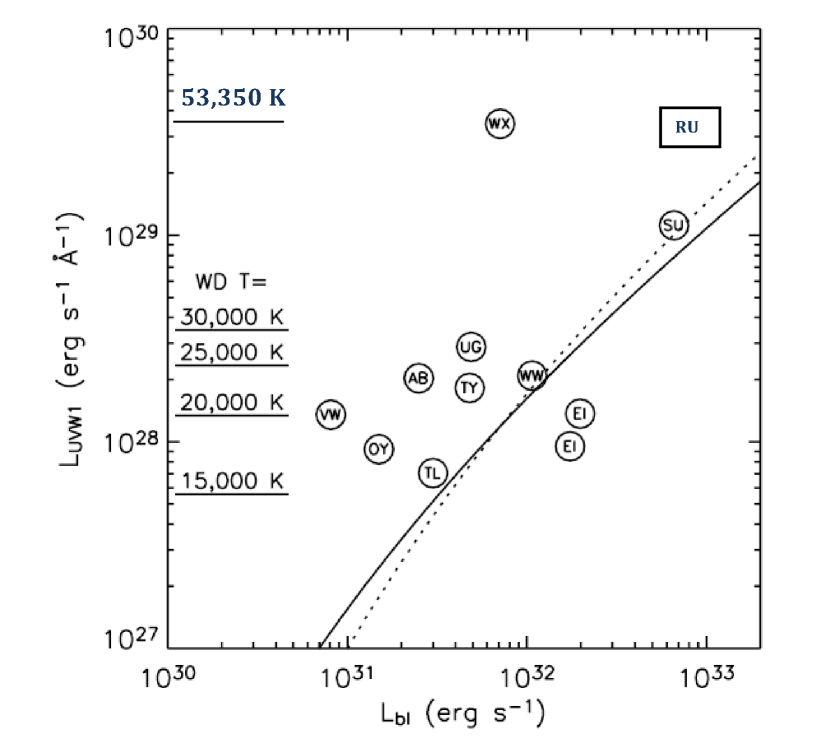
Figure 6: The boundary layer (X-ray) luminosities vs. the UV spectral luminosity at 290 nm, as derived by Pandel et al. (2005) for quiescent DNe observed with XMM-Newton. We have added RU Peg on the graph. The solid and dotted lines show $L_{bl}=L_{disk}(=L_{UVW1})$ assuming UV luminosity predicted by a simple accretion disk model for an inner radius $R_{in}=5000$ km and 10,000 km respectively. For systems higher above the line, such as RU Peg, the UV excess is due to the contribution from the WD. The UV luminosity of a WD with a 8000 km radius at various temperature is shown on the left. RU Peg corresponds here to a $\sim$53,350 K WD with a radius of 8000 km (which we have also added to the original graph), which translates to a $\sim$75,000 K for a 4000 km WD, more in line with the large mass of the WD in RU Peg. WX Hyi was caught in outburst explaining its UV excess.

The X-ray luminosity of RU Peg is $4.1\times 10^{32}$ ergs s^-1 (0.2-10.0 keV), and assuming we see only half of the boundary layer (if it is close to the star), we have $L_{bl}=8.2\times 10^{32}$ ergs s^-1. This is in the range of the other quiescent DNe observed with XMM-Newton by Pandel et al. (2005). However, in order to fully compared RU Peg with these other systems, we also need to consider the UV luminosity. For the UV we use the spectral luminosity at 290 nm $L_{UVW1}$ obtained from the OM data (see section 2.1). We have reproduced Figure 4 of Pandel et al. (2005) in Figure 6 with the inclusion of RU Peg, which shows the quiescent DNe observed with XMM-Newton plotted on a $L_{UVW1}$ against $L_{bl}$ graph. In this figure the solid and dotted lines show the relation $L_{bl}=L_{disk}$ for a UV luminosity predicted by a simple accretion disk model with an inner radius of 5000km and 10,000km respectively. This simple disk model does not include UV contribution from the WD, or outer edge of the BL where it meets the inner disk. The location of a system in the vicinity of this diagonal (e.g. SU UMa, WW Hyi) indicates that the boundary layer luminosity $L_{bl}$ is comparable to the disk luminosity (here $L_{disk}=L_{UVW1}$). For RU Peg, as for U Gem for example, the excess of UV is due to the contribution from the WD marked on the left of the graph. RU Peg has a UV luminosity corresponding to 53,350 K for a 8,000 km radius WD (assuming the flux scales simply as $\propto T^{4}$), or 75,450 K WD for a 4,000 km radius (more consistent with the large mass of RU Peg). This confirms the temperature of the WD as derived from the FUSE spectrum (Godon et al., 2008), and puts RU Peg (literally) in line with all the other quiescent DNe such as VW Hyi, U Gem, SU UMa, OY Car, and AB Dra, on the $L_{UVW1}$ versus $L_{bl}$ graph.

Because of its large mass (and therefore small radius), the WD in RU Peg has a deeper potential well, and v_Kep of the order of 5-6,000 km s^-1 in the BL. As the matter is decelerated in the BL, the X-rays emitting gas has velocities of a few 1000 km s^-1. The modeling of the O viii emission line at 19Å  implies a projected rotational broadening $v_{rot}\sin{i}=$ 695 km s^-1, i.e. the line is emitted from material rotating at $\sim$ 936-1245 km/ s^-1 (since $i\sim 34^{\circ}-48^{\circ}$) or about 1/6 of the Keplerian speed. This velocity is still much larger than the rotation speed of the white dwarf inferred from the FUSE spectrum (40 km  s^-1 ; (Godon et al., 2008)). This implies that the X-ray emission comes directly from the decelerating boundary layer material. It is possible that the X-ray emission originates in the equatorial region of the white dwarf as shown by Piro & Bildsten (2004), who found that poloidal motion may be negligible at low mass accretion rates as a characteristics of DNe in quiescence. In such a case most of the dissipated energy is radiated back into the disk, which may justify the use of a one-dimensional treatment (such as Narayan & Popham (1993); Popham (1999)).

The X-ray luminosity we computed corresponds to a boundary layer luminosity (eq.2) for a mass accretion rate of $2.0\times 10^{-11}M_{\odot}$/yr assuming a $1.29M_{\odot}$ WD mass, and it increases to $3.0\times 10^{-11}M_{\odot}$/yr for a $1.2M_{\odot}$ WD mass. This is entirely consistent with a quiescent accretion rate.

We checked the correlation between the variability of the X-ray data and the UV data and found two components; one delayed and the other undelayed. The X-ray and UV emission originate from distinct regions in the binary. Since RU Peg is a non-magnetic system, the X-ray emission is entirely from the inner edge of the boundary layer very close to the WD surface. As to the UV radiation, it is emitted by the heated WD, the very inner disk, and also that region where the outer boundary layer meets the disk (Popham, 1999). The significant modulation correlation at $\Delta t$$\sim$0 lag is expected to be caused by reprocessing of X-rays (i.e., irradiation by X-rays) in the accretion disk. Such time lags are on the order of milliseconds and proportional to light travel time which is well beyond the time resolution in our light curves. The delayed component of $\Delta t$$\sim$116 sec lag is much longer and can not be produced by light travel effects nor by reprocessing of the X-ray, since the X-ray trails behind the UV. The only viable explanation, is that the time lag is the time it takes for matter to move inwards from the very inner disk (emitting in the UV) onto the stellar surface (emitting in the X-ray). This is the time it takes to spin down the material in the boundary layer $\tau_{spin}=\Delta t=116$s . The modulations of the UV component and its lagging X-ray counterpart are due to modulations in $\dot{M}$. A comparable time delayed ($\Delta t$$\sim$100 sec) component was also detected for VW Hyi (Pandel et al., 2003), and a much shorter one ($\sim 7$s; Revnivtsev et al. 2011) was detected for the intermediate polar EX Hya (indicating that the transit of matter through magnetic field lines to the poles is faster than though the non-magnetic boundary layer).

Following the work of Godon & Sion (2005), we use the spin down time $\tau_{spin}=116$s and the rotation (or dynamical) time $\tau_{rot}=2\pi r/v_{K}(r)$=25.3s to derive the viscous time in the BL $\tau_{\nu}=\tau^{2}_{spin}/\tau_{rot}=$532s. This gives a boundary layer viscosity $\nu=\delta_{bl}^{2}/\tau_{\nu}=4.8\times 10^{13}$cm²s^-1, where we have assumed $M_{wd}=1.29M_{\odot}$, $R_{wd}=4,000$km, and a boundary layer size $\delta_{bl}$ given by the boundary layer radius $r_{bl}=(1+\delta_{bl})R_{wd}=1.4R_{wd}$ (Popham, 1999). In the alpha viscosity prescription $\nu=\alpha c_{s}H$, the value of the alpha parameter is then simply $\alpha=\nu/(c_{s}H)\approx 0.003$, where we assumed $c_{s}\approx 10^{8}$cm s^-1 (for $T\approx 10^{8}$K) and the vertical thickness of the boundary layer $H\approx 0.4R_{wd}$ (Popham, 1999). This value of $\alpha$ for the BL of RU Peg and the one derived for the BL of VW Hyi (0.009 - Godon & Sion (2005)) indicate that the alpha viscosity parameter in the BL ($\alpha_{bl}$) is much smaller than in the disk ($\alpha_{disk}$; at least in quiescent dwarf novae). This is consistent with the analytical estimates of Shakura & Sunyaev (1988) and Godon (1995) which obtained $\alpha_{bl}<<\alpha_{disk}$. Since the source of the boundary layer viscosity is unknown (Inogamow & Sunyaev, 1999; Popham & Sunyaev, 2001), this result is important for future theoretical work investigating the source of the viscosity in the boundary layer.

Table 1: XMM-Newton Observations of RU Peg

Instument	Count Rate
	$<s^{-1}>$
RGS2	$0.2881\pm 0.0030$
RGS1	$0.2351\pm 0.0029$
EPIC pn	$10.03\pm 0.017$
EPIC MOS1	$3.154\pm 0.0084$
EPIC MOS2	$3.241\pm 0.0085$

Table 2: Spectral parameters of fit to the combined EPIC spectrum of RU Peg in the energy range 0.2-10 keV. $N_{H}$ is the absorbing column, $\alpha$ is the index for power-law emissivity function ($dEM=(T/T_{max})^{\alpha-1}dT/T_{max}$), $T_{max}$ is the maximum temperature for CEVMKL model. Element names stand for the abundance relative to solar abundances, Gaussian LineE is the line center for the emission line, $\sigma_{G}$ is the line width; $K_{CEVMKL}$ and $K_{G}$ are the normalizations for CEVMKL and Gaussian models respectively. The unabsorbed X-ray flux is given in the range 0.2-10.0 keV. All error ranges are given in 90% confidence level ($\Delta\chi^{2}$=2.71 for a single parameter)

PARAMETER	VALUE
$N_{H}$ ($10^{22}$ atoms/cm2)	0.044${}^{+0.001}_{-0.001}$
$\alpha$	1.05${}^{+0.03}_{-0.03}$
$T_{max}$ (keV)	31.7${}^{+1.7}_{-2.0}$
O	0.3${}^{+0.06}_{-0.06}$
Ne	0.55${}^{+0.16}_{-0.16}$
Mg	1.3${}^{+0.2}_{-0.2}$
Si	0.8${}^{+0.14}_{-0.14}$
S	0.9${}^{+0.3}_{-0.2}$
Ca	1.8${}^{+0.8}_{-0.7}$
Fe	0.8${}^{+0.04}_{-0.04}$
$K_{CEVMKL}$	0.047${}^{+0.001}_{-0.001}$
Gaussian LineE (keV)	6.4 (fixed)
$\sigma_{G}$ (keV)	0.19${}^{+0.025}_{-0.025}$
$K_{G}$	0.000052${}^{+0.000006}_{-0.000006}$
Flux ($10^{-11}$ ergs cm-2s-1)	4.1${}^{+0.2}_{-0.2}$
$\chi^{2}_{\nu}$ (d.o.f.)	1.5 (1741)

Table 3: Line Identifications of the XMM-Newton RGS spectrum of RU Peg

Ion	Wavelength
	$<\AA>$
Mg xii	7.20
	7.45
Ne x	12.15
Fe xvii	15.03
O viii	16.05
Fe xvii	16.80
Fe xvii	17.07
O viii	19.00
O vii(i)	21.80
O vii(f)	22.11
N vii	24.77

Table 4: Spectral parameters of the fit to the RGS spectrum of RU Peg in the energy range 0.2-2.5 keV with same definitions as in Table 2.

PARAMETER	VALUE
$N_{H}$ ($10^{22}$ atoms/cm2)	0.031${}^{+0.007}_{-0.007}$
$\alpha$	1.2${}^{+0.16}_{-0.16}$
$T_{max}$ (keV)	24.1${}^{+17.0}_{-7.0}$
O	0.8${}^{+0.13}_{-0.12}$
Ne	1.1${}^{+0.5}_{-0.5}$
Mg	2.7${}^{+1.2}_{-1.1}$
Si	3.4${}^{+2.0}_{-2.0}$
S	1.4${}^{<}_{-3.2}$
Ca	1.0 (fixed)
Fe	1.0 (fixed)
$K_{CEVMKL}$	0.043${}^{+0.004}_{-0.005}$
Flux ($10^{-11}$ ergs cm-2)	3.9${}^{+0.4}_{-0.4}$
$\chi^{2}_{\nu}$ (d.o.f.)	1.3 (283)

Figure 2: Cross-correlation between X-ray and UV light curves. Left: a single Lorentzian is used to fit the data at 0; Right: a second Lorentzian fit is added to fit the delayed component. The figures show strong correlation at zero time lag. The asymmetric profile centered at zero time lag (asymmetry towards positive lag) indicates that the X-ray variations are delayed with respect to the UV variations. Error bars indicate the standard deviations from the average of the value of the cross-correlation at any given lag in different time segments where power spectra are calculated.

References

- Baskill et al. (2005) Baskill, D.S., Wheatley, P.J., Osborne, J.P. 2005, MNRAS, 357, 626
- Belloni et al. (1991) Belloni, T. et al. 1991, A&A, 246, L44
- den Herder et al. (2001) den Herder, J.W., et al. 2001, A&A, 365, L7
- Ferland et al. (1982) Ferland, G.J., Pepper, G., Langer, S.H., MacDonald, J., Truran, J.W., & Shaviv, G. 1982, ApJ, 262, L53
- Friend et al. (1990) Friend, M.T., Martin, J.S., Smith, R.C., Jones, D.H.P. 1990, MNRAS, 246, 654
- Godon (1995) Godon, P. 1995, MNRAS, 277, 157
- Godon et al. (1995) Godon, P., Regev, O., & Shaviv, G., 1995, MNRAS, 275, 1093
- Godon & Sion (2005) Godon, P., & Sion, E.M. 2005, MNRAS, 361, 809
- Godon et al. (2008) Godon, P., Sion, E.M., Barrett, P.E., Hubeny, I., Linnell, A.P., Szkody, P., ApJ, 679, 1447
- Inogamow & Sunyaev (1999) Inogamov, N.A., & Sunyaev, R.A., 1999, Astron. Lett., 25, 5.
- Jansen et al. (2001) Jansen, F. et al. 2001, A&A, 365, L1
- Johnson et al. (2003) Johnson, J.J., Harrison, T.E., Howell, S.B., Szkody, P., McArthur, B.E., Benedict, G.F. 2003, BAAS, 202, 0702
- Kennea et al. (2009) Kennea, J.A., Mukai, K., Sokoloski, J.L., Luna, G.J.M., Tueller, J., Markwardt, C.B., Burrows, D.N. 2009, ApJ, 701, 1992
- Kluźniak (1987) Kluźniak, W. 1987, Ph.D. Thesis, Standford University
- La Dous et al. (1985) La Dous, C. et al., 1985, MNRAS, 212, 231L
- Long & Gilliland (1999) Long, K.S., & Gilliland, R.L. 1999, ApJ, 511, 916
- Luna et al. (2008) Lunna, G.J.M., Sokoloski, J.L., Mukai, K. 2008, RS Ophiuchi (2006) and the Recurrent Nova Phenomenon, ASP Conferences Series, Vol. 401, p. 342, eds. A. Evans, M.F. Bode, T.J. O’brien, M.J. Darnley
- Luna & Sokoloski (2007) Luna, G.J.M. & Sokoloski, J.L. 2007, ApJ, 617, 741
- Mason et al. (2001) Mason, K.O., et al. 2001, A&A, 365, L36
- Mauche et al. (1995) Mauche, C.W., Raymond, J.C., Mattei, J.A. 1995, ApJ, 446, 842
- Mewe et al. (1985) Mewe, R., Gronenschild, E.H.B.M., & van den Oord, G.H.J. 1985, A&AS, 62, 197
- Narayan & Popham (1993) Narayan, R., & Popham, R. 1993, Nature, 362, 820
- Pandel et al. (2003) Pandel, D., Córdova, F.A., Howell, S.B. 2003, MNRAS, 346, 1231
- Pandel et al. (2005) Pandel, D., Córdova, F.A., Mason, K.O., Priedhorsky, W.C. 2005, ApJ, 626, 396
- Piro & Bildsten (2004) Piro, A.L., & Bildsten, L. 2004, ApJ, 610, 977
- Popham (1999) Popham, R. 1999, MNRAS, 308, 979
- Popham & Narayan (1995) Popham, R., & Narayan, R. 1995, ApJ, 442, 337
- Popham & Sunyaev (2001) Popham, R., & Sunyaev, R. 2001, ApJ, 547, 355
- Pringle (1981) Pringle, J.E. 1981, ARA&A, 19, 137
- Ritter & Kolb (2003) Ritter H., & Kolb U. 2003, A&A, 404, 301 http://physics.open.ac.uk/RKcat/RKcat_AA.ps
- Shafter (1983) Shafter, A. 1983, Ph.D Thesis, UCLA.
- Shakura & Sunyaev (1973) Shakura, N.I., & Sunyaev, R.A. 1973, A&A, 24, 337
- Shakura & Sunyaev (1988) Shakura, N.I., & Sunyaev, R.A. 1988, Adv.Space Res., 8, 135
- Sion et al. (1998) Sion, E.M., Cheng, F.H., Szkody, P., Sparks, W.M., Gänsicke, B.T., Huang, M., Mattei, J. 1998, ApJ, 496, 449
- Sion & Urban (2002) Sion, E.M., & Urban, J. 2002, ApJ, 572, 456
- Stover (1981) Stover, R. 1981, ApJ, 249, 673
- Strüder et al. (2001) Strüder, L., et al. 2001, A&A, 365, L18
- Szkody et al. (1991) Szkody, P., Stablein, C., Mattei, J.A., Waagen, E.O. 1991, ApJS, 76, 359
- Turner et al. (2001) Turner, M.J.L., et al. 2001, A&A, 365, L27
- Verbunt (1987) Verbunt, F. 1987, A&AS, 71, 339
- Wade (1982) Wade, R. 1982, AJ, 87, 1558
- van der Woerd & Heise (1987) van der Woerd, H., & Heise, J. 1987, MNRAS, 225, 141
- van Teeseling & Verbunt (1996) van Teeseling, A., & Verbunt, F. 1996, A&A, 292, 519