A new effective interaction for the trapped fermi gas: the BEC-BCS crossover

Abstract

We extend a recently introduced separable interaction for the unitary trapped Fermi gas to all values of the scattering length. We derive closed expressions for the interaction matrix elements and the two-particle eigenvectors and analytically demonstrate the convergence of this interaction to the zero-range two-body pseudopotential for $s$-wave scattering. We apply this effective interaction to the three- and four-particle systems along the BEC-BCS crossover, and find that their low-lying energies exhibit convergence in the regularization parameter that is much faster than for the conventional renormalized contact interaction. We find similar convergence properties of the three-particle free energy at unitarity.

I Introduction

Atomic Fermi gas systems have generated much interest in the last several years giorgini:1215 ; bloch:885 . While these systems can be well-described by a relatively simple model Hamiltonian, at low temperatures they exhibit a rich phenomenology whose theoretical description has proven to be challenging. At low momenta, or when the range of the interaction is sufficiently short, the dominant scattering process occurs in the $s$-wave channel, so that a single parameter, the $s$-wave scattering length $a$, suffices to characterize the inter-particle interaction. Depending on the value of $k_{F}a$ (where $k_{F}$ is the Fermi momentum), widely different behavior is observed. This ranges from the formation of tightly bound dimers in the Bose-Einstein condensate (BEC) regime when $k_{F}a$ is small and positive, to Cooper pairing in the Bardeen-Cooper-Schrieffer (BCS) regime when $k_{F}a$ is small and negative. These behaviors are connected by a strongly interacting, nonperturbative regime, known as the unitary regime, where $|a|$ is much larger than any other length scale in the system. Remarkably, each of these regimes is accessible experimentally, and all exhibit superfluid behavior below a certain $a$-dependent critical temperature.

While accurate mean-field theories exist for the BEC and BCS regimes, there is no simple approximation that can accurately describe the transition between these regimes through the unitary limit. As a result much interest has been taken in applying numerical methods, such as quantum Monte Carlo and numerical diagonalization. For systems varying from $\sim 10$ to hundreds of particles, quantum Monte Carlo calculations have been carried out to calculate ground state carlson:2003 ; astrakharchik:2004 ; chang:2004 ; chang:2005 ; stecher:2007 ; blume:2007 ; jauregui:2007 ; greene:2008 ; gezerlis:2008 ; zinner:2009 and thermodynamic properties bulgac:2006-9 ; burovski:2006 ; chang:2007 ; akkineni:2007 ; goulko:2010 . For smaller numbers of trapped atoms, energy spectra have been calculated using a basis set expansion method with correlated Gaussians in coordinate space (for up to six atoms) stecher:2007 ; blume:2007 and a stochastic variational approach (for four atoms) daily:2010 .

The three-body problem has been solved analytically in the unitary regime werner:2006 ; tan3body and numerically to high accuracy along the BEC-BCS crossover Kestner:2007 ; Liu:2009 . In fact the few-body trapped cold atom problem has become more interesting recently, since it was pointed out that the virial expansion for the partition function in a harmonic trap works well at unexpectedly low temperatures into the quantum degenerate regime Liu:2009 . Moreover, the scaling relations which exist for the dilute gas can allow larger systems to be addressed from the study of smaller ones adhikari:2009 ; zhang:2009 .

Here we discuss the cold atom problem in the context of the configuration-interaction (CI) approach to interacting many-particle fermionic systems. In this approach, widely used in atomic, molecular and nuclear physics, a single-particle basis in the laboratory frame is used to construct a many-particle basis of Slater determinants for a fixed number of fermions. The Hamiltonian matrix is then calculated in this many-particle basis and diagonalized. For a harmonically trapped system, a natural choice for the single-particle basis is that of the three-dimensional harmonic oscillator.

The short-range interaction of the cold atom problem is often approximated by a zero-range interaction. However, the obvious form of such a potential, a contact interaction $V_{0}\delta(\bm{r})$, is ill-defined in three dimensions and must be regularized. This is usually accomplished by introducing a momentum or energy cutoff in relative motion and renormalizing the strength $V_{0}$ of the interaction so it reproduces the physical scattering length for the uniform gas, or the lowest bound state energy in relative motion for the trapped system. The many-particle energies are then calculated as a function of the regularization cutoff parameter.

A contact interaction is non-vanishing only for relative angular momenta $l=0$ of the two particles. For a basis of harmonic oscillator wave functions, a natural regularization parameter is the number of oscillator $s$ waves in relative motion. However, the convergence of the many-particle energies as a function of this regularization parameter for the renormalized contact interaction is slow (as a low negative power) Stetcu:2008 ; Alhassid:2008 .

In Ref. Alhassid:2008, a new effective interaction was introduced in the unitary limit for which the low-lying energies of the three- and four-particle systems converge substantially faster than for the conventional renormalized contact interaction as a function of the regularization parameter. While this effective interaction is no longer a contact interaction, it reproduces the same many-particle energies in the limit when the regularization parameter is sent to infinity. The faster convergence of the many-particle energies enables their calculation to higher accuracy when using this new effective interaction. Another approach to improve the convergence relative to the renormalized contact interaction was investigated within the framework of effective field theory by including perturbatively next-to-leading order and next-to-next-to-leading order interactions Stetcu:2010 .

Here we generalize the construction of such an effective interaction away from unitarity. We study the low-energy spectra of the three- and four-particle systems and find convergence properties versus the regularization parameter along the complete BEC-BCS crossover that are similar to the unitary regime. We also use this effective interaction to study the thermodynamics of the three-particle system at unitarity. In particular, we demonstrate the exponential convergence of the free energy at finite temperature as a function of the regularization parameter. The converged free energy is compared with the exact free energy constructed from the known analytical spectrum of the three-particle system werner:2006 ; tan3body .

This paper is organized as follows. In Sec. ii@, we briefly review the two-particle cold atom problem in a harmonic trap. In Sec. iii@, we derive closed expressions for the matrix elements of the new effective interaction for any scattering length and demonstrate convergence (as a function of the regularization parameter) of its two-particle eigentates to the exact eigenstates in the unitary limit. In Sec. iv@, we use this interaction to study the convergence (vs. the regularization parameter) of the spectra of the three- and four-body systems along the BEC-BCS crossover and the three-particle free energy at unitarity. The latter is compared with exact results. Finally, in Sec. v@ we present our conclusion.

II Two-particle problem

The trapped two species cold atom system is modeled by the Hamiltonian

$$H=-\sum_{i=1}^{N}\frac{\hbar^{2}}{2m}\nabla_{i}^{2}+\sum_{i=1}^{N}\frac{1}{2}m\omega^{2}r_{i}^{2}+\sum_{i<j}V(\bm{r}_{ij}),$$ (1)

where $N=N_{1}+N_{2}$, $N_{1}$ and $N_{2}$ are the number of atoms for each species (spin-up and spin-down), $\omega$ is the trap frequency, and $V(\bm{r})$ is a short-range interaction. A natural length scale for this Hamiltonian is the oscillator length $a_{\textrm{osc}}=\sqrt{\hbar/m\omega}$.

The interaction $V(\bm{r})$ is modeled by a zero-range, pure $s$-wave interaction, which due to Pauli exclusion acts only between particles of differing species. This can be expressed by a regularized $\delta$-function,

$$V(r)=g\delta^{3}(\bm{r})(\partial/\partial r)r\;,$$ (2)

where $g=2\pi\hbar^{2}a/\mu$ relates the scattering length $a$ to the strength of the interaction giorgini:1215 . Equivalently, one can impose the Bethe-Peierls contact conditions on the wavefunctions; see, e.g., in Ref. werner:2006, . Several interesting consequences of the form (2) of the interaction potential for the many-body system have been explored in Ref. tan:2008, .

For a two-particle system, the Hamiltonian is separable in the center-of-mass and relative coordinates $\bm{R}=(\bm{r}_{1}+\bm{r}_{2})/2$ and $\bm{r}=\bm{r}_{2}-\bm{r}_{1}$, so that $H=H_{\rm CM}+H_{\rm rel}$, with

$$H_{\rm rel}=-\frac{\hbar^{2}}{2\mu}\nabla_{\bm{r}}^{2}+\frac{1}{2}\mu\omega^{2}r^{2}+V(\bm{r})\equiv H_{0}+V(r)\;,$$

where $H_{0}$ is the harmonic oscillator Hamiltonian in relative motion with reduced mass $\mu=m/2$.

The eigenstates of the non-interacting two-particle system in a harmonic trap may be labeled as $|\mathcal{NLM}nlm\rangle$, where $\mathcal{N,L,M}$ are the radial, angular momentum, and magnetic quantum numbers for the center of mass motion, and $n,l,m$ are the corresponding quantum numbers for the relative motion. The associated energies are $E=(2\mathcal{N}+\mathcal{L}+3/2+2n+l+3/2)\hbar\omega$. A pure $s$-wave interaction leaves the $l\neq 0$ states and energies unchanged while mixing the $l=0$ states into eigenstates we denote by $|\mathcal{NLM}u^{(i)}\rangle$, with $E=2\mathcal{N}+\mathcal{L}+3/2+\varepsilon_{i}$. The energies $\varepsilon_{i}$ in relative motion for scattering length $a$ are given by the solutions to the transcendental equation Busch:1998 ; Jonsell:2002

$$\frac{\Gamma(-\varepsilon/(2\hbar\omega)+3/4)}{\Gamma(-\varepsilon/(2\hbar\omega)+1/4)}=\frac{1}{\sqrt{2}a/a_{\rm osc}}.$$ (3)

The exact wave functions in relative motion are also known. They are given by Busch:1998

$$|u^{(i)}\rangle=\sum_{n=0}^{\infty}u^{(i)}_{n}|n00\rangle\;,$$

where

$$u^{(i)}_{n}=A_{i}\frac{\varphi_{n}^{\ast}(0)}{\alpha_{n}-\varepsilon_{i}}\;.$$

Here $\alpha_{n}=(2n+3/2)\hbar\omega$ are the non-interacting relative energies, $A_{i}$ is a normalization factor, and $\varphi_{n}(\bm{r})\equiv\varphi_{n00}(\bm{r})$ is a harmonic oscillator wave function, with

$$\varphi_{n}(0)=\pi^{-3/4}\left[\frac{(2n+1)!!}{(2n)!!}\right]^{1/2}\;.$$

In the unitary limit, where $\varepsilon_{i}=(2i+1/2)\hbar\omega$, the normalization factor $A_{i}$ has the simple form

$$A_{i}^{-2} = \pi^{-3/2}\sum_{n=0}^{\infty}\frac{(2n+1)!!}{(2n)!!}\frac{1}{[2(n-i)+1]^{2}}$$

$$= {\pi^{-1/2}\over 2}\frac{(2i)!!}{(2i-1)!!}\;.$$

III Effective interaction

We first discuss the conventional contact interaction. It can be regularized by introducing an energy cutoff in relative motion. This defines a sequence of interactions $\hat{V}_{\rm c}^{(q)}$, $q=0,1,2,...$, with

$$\langle nlm|\hat{V}_{\rm c}^{(q)}|n^{\prime}lm\rangle=\chi_{q}\psi_{n}(0)\psi_{n^{\prime}}(0)\delta_{l,0}\delta_{m,0}\;,$$ (4)

for $n,n^{\prime}=0,1,\ldots,q$, and where $\psi_{n}(0)\equiv[(2n+1)!!/(2n)!!]^{1/2}$. All other matrix elements of $V_{\rm c}^{(q)}$ are taken to be zero. The coefficient $\chi_{q}$ is determined for each $q$ so as to reproduce the lowest relative-motion energy $\varepsilon_{0}$. We refer to this interaction as a renormalized contact interaction.

The contact interaction in Eq. (4) is separable in the relative oscillator basis. A general separable interaction for $l=0$ has the form

$$\langle nlm|\hat{V}_{\rm eff}^{(q)}|n^{\prime}lm\rangle=f^{*}_{n}f_{n^{\prime}}\delta_{l,0}\delta_{m,0}\hskip 20.00003pt(n,n^{\prime}\leqslant q)\;.$$ (5)

An effective interaction for the trapped cold atom system can be determined by choosing the coefficients $f_{n}$ to reproduce the lowest $q+1$ relative energies $\varepsilon_{0},\ldots,\varepsilon_{q}$ of the two-particle system. This idea was used in Ref. Alhassid:2008, to construct a new effective interaction in the unitary limit of infinite scattering length. Here we consider the more general problem for any value of the scattering length $a$.

III.1 General problem and solution

The matrix elements of the relative-coordinate Hamiltonian take the form

$$\langle n00|\hat{H}^{(q)}_{\rm rel}|n^{\prime}00\rangle=\delta_{n,n^{\prime}}\alpha_{n}-f^{*}_{n}f_{n^{\prime}}\;,$$ (6)

where $\alpha_{n}$ are the non-interacting eigenvalues of $H_{0}$. To determine the coefficients $f_{n}$ we derive the following result.

Theorem. Let $\varepsilon_{0},\varepsilon_{1},\ldots,\varepsilon_{q}$ and $\alpha_{0},\alpha_{1},\ldots\alpha_{q}$ be real numbers such that $\varepsilon_{0}<\ldots<\varepsilon_{q}$, $\alpha_{0}<\ldots<\alpha_{q}$ and $\varepsilon_{i}\neq\alpha_{j}$ for all $i,j$, and let $f_{0},f_{1},\ldots,f_{q}$ be complex. Then the $(q+1)$-dimensional matrix $H_{n,n^{\prime}}=\alpha_{n}\delta_{n,n^{\prime}}-f_{n}^{*}f_{n^{\prime}}$ has the $\varepsilon_{i}$ as its eigenvalues if and only if

$$|f_{n}|=\sqrt{\frac{\prod_{k}(\alpha_{n}-\varepsilon_{k})}{\prod_{k\neq n}(\alpha_{n}-\alpha_{k})}},$$ (7)

in which case the $i$th eigenvector $b^{(i)}$ has components

$$b_{n}^{(i)}=C_{i}\frac{f_{n}^{*}}{\alpha_{n}-\varepsilon_{i}},\qquad C_{i}=\sqrt{\frac{\prod_{k}(\alpha_{k}-\varepsilon_{i})}{\prod_{k\neq i}(\varepsilon_{k}-\varepsilon_{i})}}\;.$$ (8)

A solution satisfying (7) exists if and only if $\varepsilon_{0}<\alpha_{0}<\varepsilon_{1}<\ldots<\alpha_{q}$.

Proof. An eigenvector $b^{(i)}$ with eigenvalue $\varepsilon_{i}$ must satisfy

$$\sum_{n=0}^{q}(\delta_{mn}\alpha_{n}-f_{m}^{*}f_{n})b^{(i)}_{n}=\varepsilon_{i}b^{(i)}_{m}$$ (9)

which implies

$$b^{(i)}_{n}=C_{i}\frac{f_{n}^{*}}{\alpha_{n}-\varepsilon_{i}}$$ (10)

where $C_{i}=\sum_{m}f_{m}b_{m}^{(i)}$ is a normalization constant. Inserting (10) into (9), we obtain

$$\sum_{n=0}^{q}M_{in}|f_{n}|^{2}=1\;,$$

where the matrix $M$ is defined by

$$M_{in}=\frac{1}{\alpha_{n}-\varepsilon_{i}}\;.$$ (11)

Thus the $f_{n}^{2}$ are determined from the eigenvalues by the matrix equation $M\bm{v}=\bm{1}$, where $\bm{1}=(1,1,\ldots,1)^{T}$ and $\bm{v}=(|f_{0}|^{2},|f_{1}|^{2},\ldots,|f_{q}|^{2})^{T}$.

The Matrix $M$ is of a well-known form, called a Cauchy matrix, whose inverse is given by knuthv1

$$(M^{-1})_{ni}=\frac{\prod_{k}(\alpha_{n}-\varepsilon_{k})(\alpha_{k}-\varepsilon_{i})}{(\alpha_{n}-\varepsilon_{i})\prod_{k\neq i}(\varepsilon_{k}-\varepsilon_{i})\prod_{k\neq n}(\alpha_{n}-\alpha_{k})}.$$

We therefore have

$$|f_{n}|^{2} = (M^{-1}\bm{1})_{n}$$ (12)

$$= \sum_{i}\frac{\prod_{k}(\alpha_{n}-\varepsilon_{k})(\alpha_{k}-\varepsilon_{i})}{(\alpha_{n}-\varepsilon_{i})\prod_{k\neq i}(\varepsilon_{k}-\varepsilon_{i})\prod_{k\neq n}(\alpha_{n}-\alpha_{k})}$$

$$= \frac{\prod_{k}(\alpha_{n}-\varepsilon_{k})}{\prod_{k\neq n}(\alpha_{n}-\alpha_{k})}\sum_{i}\frac{\prod_{k\neq n}(\varepsilon_{i}-\alpha_{k})}{\prod_{k\neq i}(\varepsilon_{i}-\varepsilon_{k})}\;.$$

The sum in the last expression can be evaluated using the identity knuthv1

$$\sum_{i=1}^{N}\frac{x_{i}^{r}}{\prod_{k\neq i}(x_{i}-x_{k})}=\left\{\begin{array}[]{ll}0,&0\leqslant r<N-1\\ 1,&r=N-1\\ \sum_{i=1}^{N}x_{i},&r=N\end{array}\right.$$ (13)

where $x_{1},\ldots,x_{N}$ are all distinct. This is done by observing that $\prod_{k\neq n}(\varepsilon_{i}-\alpha_{k})=\varepsilon^{q}_{i}+P(\varepsilon_{i})$, where $P$ is a polynomial of degree smaller than $q$. There are $q+1$ of the $\varepsilon_{i}$, which we take to be $x_{1},x_{2},...,x_{q+1}$ in Eqs. (13). According to the first case in Eqs. (13), the contribution to the last sum in Eq. (12) from $P(\varepsilon_{i})$ vanishes, while according to the second case of (13), the contribution of $\varepsilon^{q}_{i}$ to the sum is exactly 1. Thus, the components $f_{n}$ satisfy (7). On the other hand, it is easy to verify that if the $f_{n}$ satisfy (7) then $b^{(i)}$ given by (10) is an eigenvector with eigenvalue $\varepsilon_{i}$.

If $\varepsilon_{0}<\alpha_{0}<\varepsilon_{1}<\ldots<\alpha_{q}$ then it can easily be seen that the argument to the square root in Eq. (7) is positive, and therefore a solution for the $f_{n}$ exists. Conversely, we can show that if the argument to the square root is positive for all $n$, the eigenvalues must have this ordering. For each $n=0,\ldots,q$ let $k_{n}$ be the number of eigenvalues $\varepsilon_{i}$ for which $\varepsilon_{i}<\alpha_{n}$. Then

$$\text{sign}\,\frac{\prod_{k=0}^{q}(\alpha_{n}-\varepsilon_{k})}{\prod_{k\neq n}(\alpha_{n}-\alpha_{k})} = \frac{(-1)^{q+1-k_{n}}}{(-1)^{q-n}}.$$

In order for the sign to be positive for all $n$, we therefore require that $n+1-k_{n}$ is always even. But since $0\leq k_{0}\leq\ldots\leq k_{q}\leq q+1$, the only possibility is $k_{n}=n+1$, i.e., $\varepsilon_{0}<\alpha_{0}<\varepsilon_{1}<\ldots<\alpha_{q}$.

The eigenvectors are given by Eq. (10). To determine the normalization constant $C_{i}$, we require $\sum_{n=0}^{q}|b^{(i)}_{n}|^{2}=1$ and use Eq. (7) for $|f_{n}|$ to find

$$C_{i}^{-2} = \sum_{n=0}^{q}\frac{\prod_{0\leqslant k\leqslant q}(\alpha_{n}-\varepsilon_{k})}{\prod_{k\neq n,0\leqslant k\leqslant q}(\alpha_{n}-\alpha_{k})}\frac{1}{(\alpha_{n}-\varepsilon_{i})^{2}}.$$

This sum can also evaluated using the identity (13). To do this, we define $\alpha_{q+1}\equiv\varepsilon_{i}$ and rewrite

$$C_{i}^{-2} = \sum_{n=0}^{q}\frac{\prod_{k\neq i,0\leqslant k\leqslant q}(\alpha_{n}-\varepsilon_{k})}{\prod_{k\neq n,0\leqslant k\leqslant q+1}(\alpha_{n}-\alpha_{k})}.$$

We now add and subtract the $n=q+1$ term to obtain

$$C_{i}^{-2} = \sum^{q+1}_{n=0}\frac{\prod_{k\neq i,0\leqslant k\leqslant q}(\alpha_{n}-\varepsilon_{k})}{\prod_{k\neq n,0\leqslant k\leqslant q+1}(\alpha_{n}-\alpha_{k})}$$

$$\qquad\qquad-\frac{\prod_{k\neq i,0\leqslant k\leqslant q}(\alpha_{q+1}-\varepsilon_{k})}{\prod_{0\leqslant k\leqslant q}(\alpha_{q+1}-\alpha_{k})}.$$

Taking $x_{1}=\alpha_{0},x_{2}=\alpha_{1},...,x_{N}=\alpha_{q+1}$, the first case of (13) may be applied to find that the sum vanishes and thus

$$C_{i}^{-2} = \frac{\prod_{k\neq i}(\varepsilon_{k}-\varepsilon_{i})}{\prod_{k}(\alpha_{k}-\varepsilon_{i})}\;.$$

This completes the proof.

Since the eigenvalues $\varepsilon_{i}$, $\alpha_{n}$ for the cold atom problem are indeed ordered as the theorem requires, we choose $f_{n}=|f_{n}|$ to be positive real numbers according to Eq. (7).

The complete set of the two-particle eigenvectors of the effective interaction $V_{\rm eff}^{(q)}$ is therefore given by (i) the noninteracting states $|\mathcal{N}\mathcal{L}\mathcal{M}nlm\rangle$ for $l>0$ or ($n>q$ and $l=0$) with eigenvalues $\left(2\mathcal{N}+\mathcal{L}+3/2+2n+l+3/2\right)\hbar\omega$, and (ii) the $l=0$ interacting states

$$|\mathcal{N}\mathcal{L}\mathcal{M}b^{(i)}\rangle=\left[\frac{\prod_{k}(\alpha_{k}-\varepsilon_{i})}{\prod_{k\neq i}(\varepsilon_{k}-\varepsilon_{i})}\right]^{1/2}\\ \times\sum_{n=0}^{q}\frac{f_{n}}{\alpha_{n}-\varepsilon_{i}}|\mathcal{N}\mathcal{L}\mathcal{M}n00\rangle$$ (14)

with eigenvalues $\left(2\mathcal{N}+\mathcal{L}+3/2+\varepsilon_{i}\right)\hbar\omega$ and where the $\varepsilon_{i}$ are given by the solutions of Eq. (3).

We also derive closed expressions for the trace and norm of the $(q+1)$-dimensional matrix $V_{\rm eff}^{(q)}$ defined by $(V_{\rm eff}^{(q)})_{nn^{\prime}}\equiv\langle n00|\hat{V}_{\rm eff}^{(q)}|n^{\prime}00\rangle$. Its trace has a simple form which can be obtained via Eqs. (7) and (13). Taking $x_{1}=\alpha_{0},x_{2}=\alpha_{1},...,x_{N}=\alpha_{q}$ and applying the second and third cases of Eq. (13), we find

$$\text{tr}\ V_{\rm eff}^{(q)} = \sum_{n=0}^{q}\frac{\prod_{k}(\alpha_{n}-\varepsilon_{k})}{\prod_{k\neq n}(\alpha_{n}-\alpha_{k})}$$

$$= \sum_{n=0}^{q}(\alpha_{n}-\varepsilon_{n}).$$

This result implies that the Frobenius norm of $V_{\rm eff}^{(q)}$ is

$$\sum_{n,n^{\prime}}|(V_{\rm eff}^{(q)})_{nn^{\prime}}|^{2}=\left(\sum_{n=0}^{q}(\alpha_{n}-\varepsilon_{n})\right)^{2}\;.$$

III.2 Properties in the unitary limit

In this section we consider the properties of the separable effective interaction in the unitary limit. The simple form of the relative-motion unitary eigenvalues $\varepsilon_{i}$ allows us to verify Eq. (9) in Ref. Alhassid:2008, for the interaction parameters $f_{n}$ at unitarity and prove analytically that $V^{(q)}_{\rm eff}$ converges to the pseudopotential (2) in the limit $q\to\infty$.

III.2.1 Interaction parameters $f_{n}$

In the unitary limit $\varepsilon_{i}=2i+1/2$ are the harmonic oscillator energies shifted down by one oscillator quantum. In this case the expression for $f_{n}$ reduces to

$$f_{n}^{2} = \frac{\prod_{k=0}^{q}(2(n-k)+1)}{\prod_{k\neq n}2(n-k)}$$ (15)

$$= \frac{\prod_{k=0}^{n}(2k+1)}{\prod_{k=1}^{n}2k}\frac{\prod_{k=1}^{q-n}(-2k+1)}{\prod_{k=1}^{q-n}(-2k)}$$

$$= \frac{(2n+1)!!}{(2n)!!}\frac{(2(q-n)-1)!!}{(2(q-n))!!}\;,$$

which is exactly Eq. (9) of Ref. Alhassid:2008, .

III.2.2 Convergence of two-particle eigenvectors

To prove the convergence of the effective interaction to the pseudopotential $V({\bf r})$ in Eq. (2), we study the convergence of the two-particle eigenstates $|b^{(i)}\rangle$ of $\hat{H}_{0}+\hat{V}_{\rm eff}^{(q)}$ to the corresponding eigenstates $|u^{(i)}\rangle$ of $\hat{H}_{0}+V(r)$ as $q\rightarrow\infty$. For any scattering length, the square of the $n$-th component of $|b^{(i)}\rangle$ is given by

$$(b^{(i)}_{n})^{2} = \frac{\prod_{k}(\alpha_{k}-\varepsilon_{i})}{\prod_{k\neq i}(\varepsilon_{k}-\varepsilon_{i})}\frac{\prod_{k}(\alpha_{n}-\varepsilon_{k})}{\prod_{k\neq n}(\alpha_{n}-\alpha_{k})}\frac{1}{\left(\alpha_{n}-\varepsilon_{i}\right)^{2}}\;.$$

In the unitary case

$$(b^{(i)}_{n})^{2} = \frac{\prod_{k}(2(k-i)+1)}{\prod_{k\neq i}2(k-i)}\frac{\prod_{k}(2(n-k)+1)}{\prod_{k\neq n}2(n-k)}\frac{1}{\left(\alpha_{n}-\varepsilon_{i}\right)^{2}}$$

$$= \frac{1}{(\alpha_{n}-\varepsilon_{i})^{2}}\frac{(2i-1)!!}{(2i)!!}\frac{(2(q-i)+1)!!}{(2(q-i))!!}$$

$$\times\frac{(2n+1)!!}{(2n)!!}\frac{(2(q-n)-1)!!}{(2(q-n))!!}\;.$$

The asymptotic behavior for large $q$ is

$$b_{n}^{(i)}(q)\sim \frac{\sqrt{2/\pi}}{(\alpha_{n}-\varepsilon_{i})}\left[\frac{(2i-1)!!}{(2i)!!}\right]^{1/2}\left[\frac{(2n+1)!!}{(2n)!!}\right]^{1/2}$$

$$\times\left[\frac{q-i+3/4}{q-n+1/2}\right]^{1/4}\;.$$

We compare to the exact wave function $|u^{(i)}\rangle$ by computing the relative difference for each component,

$$\frac{|b_{n}^{(i)}-u_{n}^{(i)}|}{u_{n}^{(i)}} \sim \left|\left(1+\frac{n-i+1/4}{q-n+1/2}\right)^{1/4}-1\right|$$

$$\sim \frac{n-i+1/4}{4(q-n+1/2)}\;.$$

This diminishes like $1/q$ for large $q$, proving convergence to the exact two-body eigenstates in relative motion. Importantly, this is faster than the $1/\sqrt{q}$ convergence of the renormalized contact interaction Alhassid:2008 .

IV Applications

To demonstrate the advantage of the new effective interaction as compared with the renormalized contact interaction, we study the convergence versus $q$ of low-lying energies of the three and four-particles systems at various values of the scattering length. We also study the convergence versus $q$ of the three-particle free energy at unitarity (for which an exact solution exists). The latter is important for thermodynamical studies of the trapped gas. The three-particle system we study consists of two spin-up particles and one spin-down particle ($\uparrow\uparrow\downarrow$), while the four-particle system is unpolarized ($\uparrow\uparrow\downarrow\downarrow$).

IV.1 Spectroscopy

The CI method works in the laboratory frame and requires a certain truncation scheme. As in Ref. Alhassid:2008, , we use as our many-particle basis the set of all Slater determinants which can be constructed from the single-particle states in the harmonic oscillator shells $N=0,\ldots,N_{\rm max}$. For a given regularization parameter $q$, the two-body interaction matrix elements in the laboratory frame are calculated by transforming to the relative and center of mass coordinates via the Talmi-Moshinsky brackets Talmi:1952 and using the interaction (5) in relative motion. We carry out direct diagonalization of the CI Hamiltonian using a new code for three and four particles which works in a two-species formalism with a basis of good total orbital angular momentum $L$ and parity $\pi$. In order to determine the many-particle energies, we take the following limits. For fixed $q$ we calculate the energies as a function of $N_{\rm max}$ and extrapolate to $N_{\rm max}\to\infty$ following the method of Ref. Alhassid:2008, . The resulting energies are then studied as a function of $q$ to obtain an estimate of the $q\to\infty$ limit.

In the CI calculations we used PARPACK for parallel diagonalization on a Linux cluster using between 1 and 320 CPU cores. The largest system studied, the four-particle system with $N_{\text{max}}=12$ and total $L=1$ (involving $\sim 4.6$ million configurations), required a total of about 2300 GB to store the matrix elements of the Hamiltonian and 24 hours to run on 320 cores, while more typical calculations, e.g., four particles at $N_{\text{max}}=9$ and $L=1$ ($520,000$ configurations) required about 64 GB of storage and four hours of computation time on 32 cores.

IV.1.1 Three particles

We study a selected set of the low-lying energies of the three-particle system as a function of the inverse scattering length. Here the main topic of interest is the convergence of the eigenvalues (i) as the size of the model space (i.e., the maximal number of oscillator shells $N_{\rm max}$) increases, and (ii) as the regularization parameter $q$ increases.

(i) Overall, convergence in $N_{\rm max}$ is fast for both the renormalized contact interaction and the new effective interaction, and similar to what was already discussed in Ref. Alhassid:2008, in the unitary limit. Convergence slows somewhat as we follow the crossover from the BCS to the BEC regime and tends to require more shells as $q$ increases. At $q=4$, $N_{\rm max}=13$, we find that the lowest four eigenvalues for each of $L^{\pi}=0^{+}$, $1^{+}$, $1^{-}$, $2^{+}$, and $2^{-}$ are converged in $N_{\rm max}$ to about $0.0003\%$ in the BCS regime ($a_{\rm osc}/a=-0.8$), $0.002\%$ in the unitary limit and $0.01\%$ in the BEC regime ($a_{\rm osc}/a)=0.8$), on average.

Figure 1: Convergence of the lowest 1- state for the three particle system on either side of the crossover. The energy $E^{(q)}$ is plotted as a function of the regularization parameter $q$. Solid circles are for the effective interaction and open circles are for the renormalized contact interaction. (a): The BCS side, $a_{\rm osc}/a=-0.8$. (b): The BEC side, $a_{\rm osc}/a=+0.8$. Inset: the differences $\Delta E^{(q)}\equiv E^{(q)}-E^{(q-1)}$ on a log scale. For the effective interaction the energy decreases slightly above $q=4$, with the $q=6$ values equal to $4.7392\,\hbar\omega$ and $3.2664\,\hbar\omega$ in cases (a) and (b), respectively.

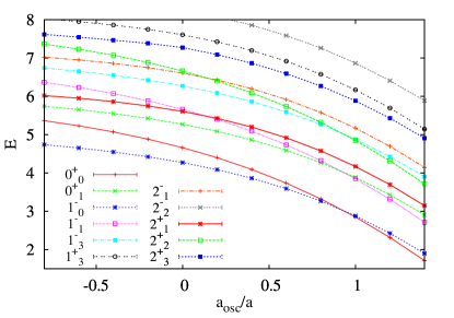
Figure 2: (Color online) Selected low-lying energies of the three-particle system vs. scattering length. Symbols are the estimates for $q\to\infty$ as described in the text. Lines are linear interpolations.

(ii) As a function of $q$ (for $1\leqslant q\leqslant 6$), we identify two convergence patterns for low-lying three-body eigenvalues. The first occurs for most eigenvalues, and is characterized by fast, monotonic convergence for $1\leqslant q\leqslant 4$ or $1\leqslant q\leqslant 5$ at an exponential or faster-than-exponential rate. The values at larger $q$ then give small, often nonmonotonic corrections. As an example, the lowest $L^{\pi}=0^{+}$ state at unitarity has the exact value $E=4.6662\ldots\hbar\omega$. With the effective interaction, we find the energy of this state decreases monotonically to $E=4.6602\,\hbar\omega$ at $q=4$ (slightly overshooting), and $E=4.6597\,\hbar\omega$ at $q=5$. The convergence then switches direction at $q=6$ and approaches the exact value with a low power-law behavior, so that the $q\geqslant 6$ values provide only a $0.14\%$ correction to the $q=4$ value. For such eigenvalues we report the energy at the highest $q$ calculated, usually $q=6$.

The second convergence pattern we encounter is completely monotonic for $2\leqslant q\leqslant 6$, but with a noticeably slower rate of convergence. For these eigenvalues, the convergence is smooth, and we estimate the $q\to\infty$ value by fitting ${\rm log}(\Delta E^{(q)})$, where $\Delta E^{(q)}=E^{(q)}-E^{(q-1)}$, to a quadratic polynomial. This provides an interpolating function $f(q)=A+Bq+Cq^{2}$ (with $C<0$) which we then use to numerically sum the residual terms in the expansion $E^{(\infty)}=E^{(q)}+\Delta E^{(q+1)}+\Delta E^{(q+2)}+\ldots\approx E^{(q)}+10^{f(q+1)}+10^{f(q+2)}+\ldots$. An example of such a state is the $0^{+}_{3}$ state at $a_{\rm osc}/a=0.0$. (We label energy levels as $L^{\pi}_{n}$, where $n$ indexes the levels with total angular momentum $L$ and parity $\pi$ in increasing order starting from zero, so that $0^{+}_{3}$ is the fourth-largest eigenvalue of those with $L=3$ and positive parity.) In this case, the $q=4$ value is $6.716\,\hbar\omega$ and the extrapolated value (from $q=6$) is $6.657$, indicating the state with the exact energy of $6.6662\ldots\hbar\omega$, a $0.14\%$ error.

Comparing with the renormalized contact interaction, we find significantly faster convergence with the new interaction for both convergence patterns. For example, the $0^{+}_{3}$ state at unitarity attains the value $6.984\,\hbar\omega$ at $q=4$ with the contact interaction, a difference of $5\%$ from the correct value, compared to $0.7\%$ at $q=4$ for the new interaction. The difference for faster-converging eigenvalues is not as dramatic, but the new interaction is still clearly preferred. This is shown in Fig. 1 for the $1^{-}_{0}$ state on either side of the crossover, at $a_{\rm osc}/a=-0.8$ and $a_{\rm osc}/a=0.8$. Importantly, we see that the advantage of the new interaction is maintained away from unitarity. This holds true for all the eigenvalues we studied, and for the four-particle system as well.

Because convergence is only truly attained for large $q$, and it is difficult to assess the effects of non-monotonicity, we estimate the systematic error in our three-particle energies along the crossover based on comparison with the unitary calculations, where we compare the convergence in $q$ with the known exact results. From this we estimate an upper bound for the systematic error due to non-convergence of approximately $0.2\%$ in our three-particle energies.

Using the new effective interaction, we also present in Fig. 2 results for a selected set of the low-lying energies of the three-particle system as a function of the inverse scattering length. Although the three-particle system is now well-studied, this provides a clear verification of the capability of the method. Our results agree with those published previously Stetcu:2008 ; Kestner:2007 . As in the the earlier studies, we find crossings between levels with different quantum numbers, for instance the $2^{+}_{1}$ state and the $1^{-}_{1}$ state at approximately $a_{\rm osc}/a=0.14$, and the $1^{-}_{0}$ state and the $0^{+}_{0}$ state at approximately $a_{\rm osc}/a=0.93$, which changes the parity and angular momentum of the ground state.

IV.1.2 Four particles

The four-particle system is less well-studied and provides a more interesting test of the new effective interaction. As with the three-particle system, we examined a selected set of the low-lying energies as a function of the inverse scattering length.

(i) Overall we find fast convergence in $N_{\rm max}$, very similar to the three-particle case. More precisely, at $q=4$, $N_{\rm max}=11$, the level of convergence ranges from an average of about $0.05\%$ at $a_{\rm osc}/a=-0.8$ to $0.2\%$ at $a_{\rm osc}/a=0.8$ for the lowest four states of each of the $0^{-}$, $0^{+}$, $1^{-}$ and $1^{+}$ configurations.

(ii) As a function of $q$, the two convergence patterns observed for the three particle case – the more common fast, slightly non-monotonic convergence and the less common slower, monotonic convergence – are still prevalent, but with the addition of a few eigenvalues which are non-monotonic for smaller $q$. An example is the $0^{+}_{1}$ state at unitarity, which becomes non-monotonic at $q=3$. For eigenvalues with the first two convergence patterns, we estimate the $q\to\infty$ values in the same manner as the three-particle case. For the new non-monotonic eigenvalues, we report the result of the calculation at largest $q$, usually $q=5$. For instance, for the $0^{+}_{1}$ state at unitarity, the $q=5$ value is $E=7.036\,\hbar\omega$, and appears to be an upper bound based on the direction of convergence. This compares favorably with the result $E=7.010\,\hbar\omega$ (a $0.4\%$ difference) of Ref. daily:2010, , in which the center of mass coordinate is separated out and a stochastic variational approach is employed. Note we add a center of mass excitation of $1.5\,\hbar\omega$ to the results of Ref. daily:2010, to allow comparison.

An example of a fast, slightly non-monotonic energy is the $1^{+}_{0}$ state, which was calculated in Ref. daily:2010, to have a value $E=6.588(20)\,\hbar\omega$. Our $q=5$ estimate of the new interaction is $6.582\,\hbar\omega$, well within error.

Compared with the renormalized contact interaction, the new interaction provides much improved convergence for four particles, as it did for the three particle system. For example, Fig. 3 shows the convergence of the $1^{+}_{0}$ state using the new and the renormalized contact interactions on either side of the crossover. As with all the energies we have studied, this displays a marked improvement in convergence. On the BEC side, in particular, we find a $7\%$ difference between the two interactions at $q=4$.

Figure 3: Convergence of the lowest $1^{+}$ state for the four particle system. Solid circles are the results calculated with the effective interaction, and open circles are the results from the renormalized contact interaction. (a): Convergence of the energy $E^{(q)}$ vs $q$ on the BCS side of the crossover at $a_{\rm osc}/a=-0.8$. (b): The BEC side of the crossover at $a_{\rm osc}/a=+0.8$. Inset: The absolute values of the differences $|\Delta E^{(q)}|$. In both cases, the convergence becomes slightly non-monotonic at the $q=5$ point.

In Fig. 4 we present results for a selected set of low-lying energies of the four-particle system as a function of inverse scattering length. As for the three-particle case, we find crossings between levels with different quantum numbers, for instance, the $1^{+}_{1}$ state and the $0^{-}_{0}$ state at approximately $a_{\rm osc}/a=0.36$. In contrast to the three-particle system, the angular momentum and parity of the ground state (here $0^{+}_{0}$) remain fixed through the full range of scattering lengths.

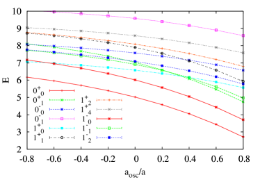
Figure 4: (Color online) Selected low-lying energies of the four-particle system vs. scattering length. Symbols are the estimates for $q\to\infty$ as described in the text. Lines are linear interpolations.

IV.2 Thermodynamics

As thermodynamics is one of the central topics of interest for cold atoms, we test the usefulness of the new separable effective interaction for thermodynamical studies by studying the convergence of the free energy (at a given temperature) versus $q$ for the three-particle system. Our calculations were done at temperatures between $T=0\,\hbar\omega$ and $T=2.0\,\hbar\omega$ as a function of $q$ and $N_{\rm max}$ via a direct diagonalization of the Hamiltonian through $N_{\rm max}=10$. We compare our calculations with exact results for the three-particle system.

An example of the convergence in $N_{\rm max}$ for $q=4$ and $T=0.4\,\hbar\omega$ is shown in Fig. 5, where we observe smooth behavior for both interactions. For higher temperatures, the smooth character of the $\Delta F$ vs. $N_{\rm max}$ is preserved, while the curvature flattens out to a straight line (on a logarithmic scale), allowing for accurate extrapolations in $N_{\rm max}$.

The convergence as a function of $q$ is demonstrated in the inset to Fig. 6 for $T=0.4\;\hbar\omega$. The convergence using the new effective interaction is significantly faster than for the renormalized contact interaction. In general, we found that the convergence in $q$ for the new interaction was quite uniform and fast for temperatures up to approximately $T=1.0\,\hbar\omega$. In fact, at higher temperatures, the abundance of interactionless states (see below) diminishes the error for even small $q$ values so that at $T=2.0\,\hbar\omega$, the difference between $q=1$ and the exact value is only about $0.8\%$, compared to $2.1\%$ at $T=0.1\,\hbar\omega$. By comparison, the difference in the free energy between the non-interacting and interacting systems is $2\%$ at $T=2.0\,\hbar\omega$ and $30\%$ at $T=0.1\,\hbar\omega$.

Figure 5: Convergence of the free energy in $N_{\rm max}$ at $T=0.4\hbar\omega$ and $q=4$ calculated with the effective interaction (solid circles) and renormalized contact interactions (open circles). The solid lines are fits to the interpolating function ${\rm log}(\Delta F)=A+Bq+Cq^{2}$ with fit parameters $A$,$B$,$C$, and are used to extrapolate to the limit $N_{\rm max}~{}\to~{}\infty$.

Our thermodynamics studies are summarized in Figs. 6 and 7, where we compare our calculations of the free energy and entropy as a function of temperature with exact calculations for the interacting and non-interacting systems (described below). We find excellent agreement. Although this is only a three-body system, the entropy curve indicates that our results apply in the entirety of the interesting quantum degenerate regime.

Figure 6: Free energy versus temperature for the three-particle system. Solid circles: new effective interaction at $q=4$. Solid line: exact result. Dashed line: non-interacting system. The inset demonstrates the convergence of $F$ vs. $q$ at $T=0.4\,\hbar\omega$. The solid circles were calculated using the separable effective interaction, while the open circles are from the renormalized contact interaction. The horizontal line indicates the exact result of $3.6537\ldots\hbar\omega$.

Figure 7: Entropy versus temperature for the three-particle system, calculated via a numerical derivative of the free energy, $S=-\partial F/\partial T$. Symbols and lines are as in Fig. 6.

Since the three-body problem has been solved exactly at unitarity werner:2006 ; tan3body , we can compare the thermodynamic functions calculated using the new effective interaction with exact results.

We summarize the exact calculation as follows. There are two classes of eigenstates for the trapped Fermi gas, interacting states and interactionless states. The interacting states satisfy the Bethe-Peierls contact condition werner:2006

$$\varphi(\bm{r}_{1},\bm{r}_{2},\bm{r}_{3})=\left(\frac{1}{r_{ij}}-\frac{1}{a}\right)A(\bm{R}_{ij},\bm{r}_{k})+O(r_{ij})$$

(as $r_{ij}\rightarrow 0$) via a function $A$ which is non-zero. The interactionless states satisfy a similar condition but with $A$ identically zero. They are also eigenstates of the non-interacting Hamiltonian and are identical for all values of the scattering length.

To calculate the energy levels of the interacting states we follow the procedure of Ref. werner:2006, . However, as noted there, at large temperatures the number of interactionless states grows much larger than that of the interacting states, so that energies for both are necessary to calculate thermodynamic quantities for the system. The wave functions and energies of the interactionless states for the three-particle system have been characterized completely in Ref. tan3body, . Below we summarize the main results.

The energy of any state of the system (interacting or interactionless) is given by

$$E=(\gamma+n_{c}+2\nu+9/2)\hbar\omega$$

where $n_{c}$ is the number of oscillator quanta in the center-of-mass excitation, $\gamma$ is a scaling exponent, and $\nu=0,1,2,...$ is the hyperradial quantum number. The corresponding intrinsic wave functions are of the form $\psi\propto\tilde{\phi}\,L_{\nu}^{(\gamma+2)}(R^{2}/a_{\rm osc}^{2})e^{(-R^{2}/2a_{\rm osc}^{2})}$, where $R$ is the hyperradius. The function $\tilde{\phi}$ ($\propto R^{\gamma}$) satisfies the Bethe-Peierls contact conditions as well as additional equations. States with total internal angular momentum $l=0,1,\ldots$ have exponents $\gamma_{l,n}$ where $n=0,1,\ldots$. For the interacting states $\gamma_{l,n}=s_{l,n}-7/2$ where $s_{l,n}$ are an infinite sequence of solutions to an $l$-dependent transcendental equation obtained from the three-particle Schrodinger equation werner:2006 . For the interactionless states, $\gamma_{l,n}$ are integers $\geq 2$ and have degeneracies; these degeneracies are non-trivial and must be determined in order to calculate thermodynamic quantities for the system. We followed the method of Ref. tan3body, to determine these degeneracies (see, e.g., Table II of Ref. tan3body, ).

Using the above classification of interacting and interactionless states, we computed the entire three-body spectrum to the extent needed to ensure convergence of the free energy at any temperature of interest (see Figs. 6 and 7). Table 1 provides a few values of the free energy $F$ and entropy $S$ at various temperatures for reference. For the non-interacting calculations we use simple closed formulas that are derived in the Appendix.

$T\,\,(\hbar\omega)$	$E\,\,(\hbar\omega)$	$F\,\,{\bf(\hbar\omega)}$	$S$	$E_{\text{free}}$	$F_{\text{free}}$	$S_{\text{free}}$
0.1	4.2754	4.1622	1.1321	5.5003	5.3901	1.1016
0.5	5.0767	3.3510	3.4514	6.5632	4.4837	4.1590
1.0	8.5107	0.47585	8.0348	10.017	1.1690	8.8483
2.0	17.792	-11.109	14.451	18.459	-10.874	14.667

Table 1: A few values of the exact thermodynamic functions of the unitary and non-interacting three-particle systems. $E$, $F$, and $S$ are the energy, free energy and entropy of the unitary system; $E_{\text{free}}$, $F_{\text{free}}$, and $S_{\text{free}}$ are the same quantities for the non-interacting system.

V Conclusion

We have extended a new separable effective interaction for the unitary trapped gas in the configuration-interaction framework to regions away from unitarity, i.e., the BEC-BCS crossover. The main advantage of this interaction, when compared with the conventional renormalized contact interaction, is its much improved convergence of the many-particle energies in the regularization parameter. This allows accurate calculations in the configuration interaction approach. In particular, we calculated the low-lying energies for three and four particles as a function of the inverse scattering length.

We also studied the three-particle system at finite temperature in the unitary limit and found similar convergence properties of the free energy as a function of the regularization parameter. This separable effective interaction may therefore facilitate accurate studies of the thermodynamics of the trapped cold atom system.

Appendix A Non-interacting thermodynamics

In Figs. 6 and 7 we compared our calculations with the non-interacting three-body trapped systems (dashed lines). For this purpose we derived simple formulas for the canonical partition functions of small systems of trapped non-interacting spin-$1/2$ particles. For three particles ($\uparrow\uparrow\downarrow$), we proceed as follows. Label the state of each particle as $\bm{s}=(n_{x},n_{y},n_{z},\sigma)$, where $n_{x},n_{y},n_{z}$ are the $3$-D harmonic oscillator quantum numbers and $\sigma=\pm 1/2$ is the $z$-component of the spin. Then the canonical partition function is

$$\mathcal{Z}=\frac{1}{3!}\sum_{\begin{subarray}{c}\bm{s}_{1},\bm{s}_{2},\bm{s}_{3}\\ \sigma_{1}+\sigma_{2}+\sigma_{3}=1/2\end{subarray}}e^{-\beta\left(E_{\bm{s}_{1}}+E_{\bm{s}_{2}}+E_{\bm{s}_{3}}\right)}S(\bm{s}_{1},\bm{s}_{2},\bm{s}_{3})$$

where $E_{\bm{s}}=(n_{x}+n_{y}+n_{z}+3/2)\hbar\omega$ and $S(\bm{s}_{1},\bm{s}_{2},\bm{s}_{3})$ is the selection function

$$S(\bm{s}_{1},\bm{s}_{2},\bm{s}_{3}) =\left\{\begin{array}[]{l l}0&\quad\mbox{if any two $\bm{s}_{i}$ are equal}\\ 1&\quad\mbox{otherwise}\\ \end{array}\right.$$ (18)

$$=\prod_{i<j}(1-\delta_{\bm{s}_{i},\bm{s}_{j}}).$$ (19)

To perform the sum, one expands the selection function to obtain eight terms involving sums over the Maxwell-Boltzmann factor $e^{-\beta\left(E_{\bm{s}_{1}}+E_{\bm{s}_{2}}+E_{\bm{s}_{3}}\right)}$ times a product (say $D$) of zero to three Kronecker $\delta$’s. By collapsing the sum over the $\delta$’s one obtains a geometric series which then easily yields a closed-form expression. As an example, for $D=\delta_{\bm{s}_{1},\bm{s}_{2}}$, and with the notation $|\bm{n}_{i}|\equiv n_{i,x}+n_{i,y}+n_{i,z}$, the corresponding sum is

$$\begin{split}\sum_{\begin{subarray}{c}\bm{s}_{1},\bm{s}_{2},\bm{s}_{3}\\ \sigma_{1}+\sigma_{2}+\sigma_{3}=1/2\end{subarray}}&e^{-\beta\left(E_{\bm{s}_{1}}+E_{\bm{s}_{2}}+E_{\bm{s}_{3}}\right)}\delta_{\bm{s}_{1},\bm{s}_{2}}\\ &=\left(\frac{1}{1-e^{-2\beta}}\right)^{3}\left(\frac{1}{1-e^{-\beta}}\right)^{3}.\end{split}$$

Note that in this case, the sum over $\sigma_{2}$ and $\sigma_{3}$ is exactly 1 (and is zero for the two and three-$\delta$ terms for this system).

The final result is

$$\@ADDCLASS{ltx_eqn_lefteqn}$\displaystyle\mathcal{Z}=\frac{1}{2}e^{-9\beta/2}\Bigg{[}\left(\frac{1}{1-e^{-\beta}}\right)^{9}-$\mbox{}\hfil\\ \left(\frac{1}{1-e^{-\beta}}\right)^{3}\left.\left(\frac{1}{1-e^{-2\beta}}\right)^{3}\right].$$

References

- (1) I. Bloch, J. Dalibard, and W. Zwerger, Rev. Mod. Phys. 80, 885 (2008).
- (2) S. Giorgini, L. P. Pitaevskii, and S. Stringari, Rev. Mod. Phys. 80, 1215 (2008).
- (3) Q. Chen, J. Stajic, S. Tan, and K. Levin, Phys. Rep. 412, 1-88 (2005).
- (4) J. Carlson, S.-Y. Chang, V. R. Pandharipande, and K. E. Schmidt, Phys. Rev. Lett. 91, 050401 (2003).
- (5) G. E. Astrakharchik, J. Boronat, J. Casulleras, and S. Giorgini, Phys. Rev. Lett. 93, 200404 (2004).
- (6) S. Y. Chang, V. R. Pandharipande, J. Carlson, K. E. Schmidt, Phys. Rev. A 70, 043602 (2004).
- (7) S. Y. Chang and V. R. Pandharipande, Phys. Rev. Lett. 95, 080402 (2005).
- (8) J. von Stecher, C. H. Greene, and D. Blume, Phys. Rev. A 76, 053613 (2007).
- (9) D. Blume, J. von Stecher, and C. H. Greene, Phys. Rev. Lett. 99, 233201 (2007).
- (10) R. Jáuregui, R. Paredes, and G. T. Sánchez, Phys. Rev. A 76, 011604(R) (2007)
- (11) J. von Stecher, C. H. Greene, and D. Blume, Phys. Rev. A. 77, 043619 (2008)
- (12) A. Gezerlis and J. Carlson, Phys. Rev. C 77, 032801(R) (2008)
- (13) N. T. Zinner, K. Mølmer, C. Özen, D. J. Dean, and K. Langanke, Phys. Rev. A 80, 013613 (2009).
- (14) A. Bulgac, J. E. Drut, and P. Magierski, Phys. Rev. Lett. 96, 090404 (2006); Phys. Rev. Lett. 99, 120401 (2007); Phys. Rev. A 78, 023625 (2008); P. Magierski, G. Wlazlowski, A. Bulgaac, and J. E. Drut, Phys. Rev. Lett. 103, 210403 (2009).
- (15) E. Burovski, N. Prokof’ev, B. Svistunov, and M. Troyer, Phys. Rev. Lett. 96, 160402 (2006).
- (16) S. Y. Chang and G. F. Bertsch, Phys. Rev. A 76, 021603(R) (2007).
- (17) V. K. Akkineni, D. M. Ceperly, and N. Trivedi, Phys. Rev. B 76, 165116 (2007).
- (18) O. Goulko and M. Wingate, Phys. Rev. A 82, 053621 (2010).
- (19) K. M. Daily and D. Blume, Phys. Rev. A 81, 053615 (2010); D. Blume and K. M. Daily, arXiv:1008.3191.
- (20) F. Werner and Y. Castin, Phys. Rev. Lett. 97, 150401 (2006).
- (21) S. Tan, preprint (2006) and private communication.
- (22) J. P. Kestner and L.-M. Duan, Phys. Rev. A 76, 033611 (2007).
- (23) X.-J. Liu, H. Hu, and P. D. Drummond, Phys. Rev. Lett. 102, 160401 (2009); Phys. Rev. A 82, 023619 (2010).
- (24) S. K. Adhikari, Phys. Rev. A 79, 023611 (2009)
- (25) S. Zhang and A. J. Legget, Phys. Rev. A 79, 023601 (2009)
- (26) I. Stetcu, B. R. Barrett, U. van Kolck, and J. P. Vary, Phys.Rev. A 76, 063613 (2007).
- (27) Y. Alhassid, G. F. Bertsch, and L. Fang, Phys. Rev. Lett. 100, 230401 (2008).
- (28) I. Stetcu, J. Rotureau, B.R. Barrett, U. van Kolck, arXiv:1001.5071; J. Rotureau, I. Stetcu, B. R. Barrett, M. C. Birse, and U. van Kolck, Phys. Rev. A 82, 032711 (2010).
- (29) S. Tan, Ann. Phys. (N.Y.) 323, 2952 (2008); Ann. Phys. (N.Y.) 323, 2971 (2008); Ann. Phys. (N.Y.) 323, 2987 (2008).
- (30) S. Jonsell, Few-Body Systems 31, 255 (2002).
- (31) T. Busch, B.-G. Englert, K. Rza̧żewski, and M. Wilkens, Found. Phys. 28, 549 (1998).
- (32) D. E. Knuth, The art of computer programming, vol. 1, fundamental algorithms, (Addison-Wesley, 1997) pp. 36-38, 3rd ed.
- (33) I. Talmi, Helv. Phys. Acta 25, 185 (1952); M. Moshinsky, Nucl. Phys. 13, 104 (1959).