Dipolar response of hydrated proteins

Abstract

The paper presents an analytical theory and numerical simulations of the dipolar response of hydrated proteins. The effective dielectric constant of the solvated protein, representing the average dipole moment induced at the protein by a uniform external field, shows a remarkable variation among the proteins studied by numerical simulations. It changes from 0.5 for ubiquitin to 640 for cytochrome c. The former value implies a negative dipolar susceptibility of ubiquitin, that is a dia-electric dipolar response and negative dielectrophoresis. It means that a protein carrying an average dipole of $\simeq 240$ D is expected to repel from the region of a stronger electric field. This outcome is the result of a negative cross-correlation between the protein and water dipoles, compensating for the positive variance of the protein dipole in the overall dipolar susceptibility. This phenomenon can therefore be characterized as overscreening of protein’s dipole by the hydration shell. In contrast to the neutral ubiquitin, charged proteins studied here show para-electric dipolar response and positive dielectrophoresis. The protein-water dipolar cross-correlations are long-ranged, extending approximately 2 nm from the protein surface into the bulk. A similar correlation length of about 1 nm is seen for the electrostatic potential produced by the hydration water inside the protein. The analysis of numerical simulations suggests that the polarization of the protein-water interface is strongly affected by the distribution of the protein surface charge. This component of the protein dipolar response gains in importance for high frequencies, above the protein Debye peak, when the response of the protein dipole becomes dynamically arrested. The interface response found in simulations suggests a possibility of a positive increment of the high-frequency dielectric constant of the solution compared to the dielectric constant of the solvent. This analysis provides a theoretical foundation for experimentally observed positive increments of the absorption of THz radiation by protein solutions.

I Introduction

Polarization of the interface is an important component of the response of a polar substance to an external field. The standard approach of Maxwell’s electrostatics assumes that the interface cuts through the polarized dipoles of the dielectric, leaving their monopoles at the surface (Fig. 1a). The density of these monopoles is the surface charge density $\sigma_{P}$. It is given by the projection $P_{n}$ of the dipolar polarization vector $\mathbf{P}$ on the outward normal $\mathbf{\hat{n}}$ to a continuous dielectric medium.Landau8 ; Frohlich This surface charge is opposite in sign to an external charge and so the field of the surface charges compensates the external field. The sum of the two fields makes the Maxwell field inside the dielectric, which is lower in intensity than the external field.

The same basic considerations apply to the problem of solutions polarized by a uniform external field $\mathbf{E}_{0}$. The interface is now a closed surface enveloping each solute. The polarization field, uniform in the bulk, becomes inhomogeneous close to the solute-solvent interface. It generates positive and negative lobes of the surface charge density (Fig. 2) integrating into an overall interface (subscript “int”) dipole $\mathbf{M}_{0}^{\text{int}}$. Its calculation is generally a complex problem involving both the effects of the solute shape and the alteration of the liquid structure by the solute surface multipoles. A closed-form solution is, however, possible in the framework of standard dielectric theories for a spherical void in a dielectric,Landau8 when all specifics of the solute-solvent interactions are neglected

$$\mathbf{M}_{0}^{\text{int}}=-3\Omega_{0}\mathbf{P}/(2\epsilon_{s}+1).$$ (1)

Here, $\epsilon_{s}$ is the solvent dielectric constant, $\Omega_{0}$ is the solute volume, and subscript “0” is assigned throughout below to the solute parameters. The orientation of the interface dipole is opposite to the uniform polarization of the medium $\mathbf{P}$.

The appearance of $\mathbf{M}_{0}^{\text{int}}$ is an interfacial, but not necessarily a surface phenomenon. This interface dipole is the integral effect of the inhomogeneous polarization surrounding an excluded volume of the solute. This polarization perturbation in fact propagates quite far into the bulk, as we show below, and can be taken fully into account only in the thermodynamic limit for the solution, which we represent below as the $k\rightarrow 0$ limit in the inverted Fourier space of wavevectors $\mathbf{k}$. The surface charge density $\sigma_{P}$ is just a convenient mathematical representation of this highly non-local physical reality in terms of properties assigned to an infinitely thin mathematical surface enveloping the solute.

The interface dipole arising from a void in a uniformly polarized liquid will in turn polarize the surrounding solvent. As a result, the dipole moment of a uniformly polarized solution is given as

$$\mathbf{M}_{s}=\mathbf{M}^{\text{liq}}-\Omega_{0}\mathbf{P}-(2/3)(\epsilon_{s}-1)\mathbf{M}_{0}^{\text{int}}.$$ (2)

The first summand in this equation is the dipole moment of a uniformly polarized homogeneous liquid. The second term is the dipole moment reduced from the liquid by putting a solute of volume $\Omega_{0}$ into it. Finally, the last summand is the polarization of the liquid by the interface dipole.

The interface dipole $\mathbf{M}_{0}^{\text{int}}$ exists at any closed interface in a polarized medium, even in the absence of solute’s own charges. When calculated according to Eqs. (1) and (2), it will lower the dielectric constant of the solution $\epsilon$ compared to the dielectric constant $\epsilon_{s}$ of the homogeneous liquid. In contrast, if the solute possesses its own dipole, it will align along the external field $E_{0}$ producing an average permanent dipole $\langle\mathbf{M}_{0}\rangle_{E}$. This dipole moment will enhance the dielectric response of the solution. The overall dipole moment associated with a solute will be the sum of the intrinsic permanent dipole and the dipole induced at the dielectric interfaceDMpre:10

$$\mathbf{M}_{0}=\langle\mathbf{M}_{0}\rangle_{E}+\mathbf{M}_{0}^{\text{int}},$$ (3)

where $\langle\dots\rangle_{E}$ refers to the statistical average in the presence of the field.

Both the permanent and interface components of $\mathbf{M}_{0}$ depend on the ability of the interface to polarize. The very basic physics outlined in Fig. 1a assumes the dipoles of the medium to have the ability to freely change their orientations in order to align along an external electric field. While this is probably the case for solvation of small ions in polar liquids, solvation of larger solutes might present a challenge to this picture.

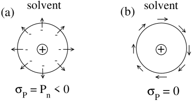
Figure 1: Cartoon of two extreme polarization patterns of a polar solvent at the surface of a spherical solute with a positive charge at the center. In panel (a), the solvent dipoles align with the electric field of the solute charge. This alignment results in surface charge density $\sigma_{P}=P_{n}<0$. In panel (b), the surface dipoles preserve their preferential in-plane orientations characteristic of a free surface of a polar liquid.Sokhan:97 This orientational pattern produces no surface charge, $\sigma_{P}=0$.

Dipoles of polar liquids preferentially orient in-plane at interfaces.Lee:84 ; Sokhan:97 ; Bratko:09 ; DMepl:08 ; Rossky:10 ; DMjcp2:11 Unless an external field rotates the dipoles off-plane, such orientational structure eliminates the surface charge since $\sigma_{P}=P_{n}\simeq 0$ in this case (Fig. 1b). The standard boundary conditions of continuum electrostatics do not apply to this scenario which implies

$$\mathbf{M}_{0}^{\text{int}}=0,$$ (4)

instead of the standard electrostatic result listed in Eq. (1).

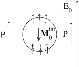
Figure 2: Cartoon of the interface polarization of a spherical void in a uniformly polarized polar liquid. The surface charges at the interface produce negative and positive lobes of the overall surface charge density responsible for the interface dipole $M_{0z}^{\text{int}}=\chi_{1}\Omega_{0}E_{0}$. When the surface charge density disappears because of the in-plane alignment of the surface dipoles, the dipole subtracted from the solution is simply the product of the solute volume and the uniform polarization of the bulk [Eq. (2)]. This is the Lorentz scenario of the interface polarization corresponding to $\chi_{1}=0$. In contrast, the Maxwell scenario anticipates a non-zero surface charge density, which reduces the dipole taken from the solution from the Lorentz value $-P_{z}\Omega_{0}$ to the Maxwell value given by Eq. (1). This scenario also anticipates a nonzero and negative dipolar interface susceptibility $\chi_{1}$ given by Eq. (15).

Equations (2) and (4) suggest that carving a void from a dielectric removes the dipole moment equal to the product of the uniform bulk polarization and the void volume. Such a solution would appear in the standard theories of dielectricsScaife:98 if the void in the dielectric had the interface of a Lorentz virtual cavity, which has no surface polarization by definition. We will dubb this outcome, corresponding to $\sigma_{P}=0$ in Fig. 1b, as the “Lorentz scenario”. On the other hand, when $\mathbf{M}_{0}^{\text{int}}$ from Eq. (1) is substituted into Eq. (2), the two last terms combine into the same $\mathbf{M}_{0}^{\text{int}}$, which becomes the dipole subtracted from the homogeneous liquid upon insertion of the solute. The rules of electrostatics therefore predict that the dipole removed from the solution will be, at $\epsilon_{s}\gg 1$, just a small fraction of the Lorentz dipole. Since this scenario follows from the standard electrostatics with Maxwell’s boundary conditions at the dielectric interface, we will call this outcome, and the corresponding interface polarization, the “Maxwell scenario” (Figs. 1a and 2).

Water presents a particularly important study case for the Lorentz scenario of Eq. (4). Large solutes, over 1 nm in size,ChandlerNature:05 ; Ball:08 break the network of hydrogen bonds of bulk water, resulting in preferential in-plane orientation of the interfacial water dipoles.Lee:84 ; Sokhan:97 ; Bratko:09 ; Rossky:10 This phenomenon, general for polar fluids,DMepl:08 ; DMpre1:08 is further amplified for water interfaces by the high energy of water’s hydrogen bonds.DMjcp2:11

The orientational structure of interfacial water has macroscopically observable consequences, both mechanical and electrostatic. Mechanical consequences include the rotation of hydrated nanometer solutes by external fields Daub:09 and slipping of the boundary layers in the hydrodynamic flow.Barrat:99 For electrostatic observables, the electric field inside cavities formed in uniformly polarized dipolar liquidsDMepl:08 and in waterDMjcp2:11 seem to follow the scenario of an unpolarized interface sketches in Fig. 1b. One can therefore anticipate that in-plane dipolar orientations might be preserved, at least in patches, if the external field is not sufficiently strong to compete with interface hydrogen bonds forcing water dipoles orient in-plane. If this is the case, the boundary conditions of the dielectric response problem will alter, thus affecting all relevant polar response functions.

Electrostatic interactions are critical for biological function.Tessier:03 ; Gitlin:06 ; Warshel:06 Most biomolecules and all cellular membranes carry charges.Sear:03 Electrostatic solvation and interactions affect the stability of folded proteins and their aggregation and crystallization. Richardson:02 ; Lawrence:07 ; Pace:09 Therefore, the question of what is the dipolar polarization at the interface of a hydrated biomolecule is critical for structural biology and bioenergetics.DMpccp:10

Surfaces of proteins, and of all biomaterials in general, are obviously chemically and electrostatically heterogeneous.Giovambattista:08 One therefore cannot expect a clear-cut scenario of either in-pane dipoles or dipoles fully aligned along the electric field. This study in fact shows that none of the scenarios sketched in Fig. 1 presents a complete description of hydrated proteins, which explore a much wider range of possibilities allowing them to tune their response to global and local in vitro fields. To grasp this complexity, we ask what would be a minimal set of coarse-grained parameters describing the water-protein interface. We approach this question here by first presenting an analytical theory framing the problem in terms of a set of interface susceptibilities, followed by numerical simulations of several hydrated globular proteins. The property of interest is the average dipole moment $M_{0}$ [Eq. (3)] induced at the protein by an external electric field. As such, this is a fundamental and well-defined physical quantity related to broad-band dielectric spectroscopy of solutions, not considered here, and directly probed by dielectrophoresis of protein solutionsWashizu:94 ; JonesBook:95 ; HughesBook:03 discussed below.

II Dielectric considerations

According to the separation of the solute dipole into the intrinsic permanent and interfacial components, one can define linear dipolar susceptibilities for the corresponding dipoles along the external field. If the $z$-axis of the laboratory frame is set along the external field, one gets for the dipolar (“d”) and interfacial (“int”) parts of the response

$$\begin{split}&\chi_{0}^{d}=\langle M_{0z}\rangle_{E}/(\Omega_{0}E_{0}),\\ &\chi_{0}^{\text{int}}=M_{0z}^{\text{int}}/(\Omega_{0}E_{0}).\end{split}$$ (5)

We first focus on the solute permanent dipole and consider the first-order perturbation expansion for the corresponding susceptibilityFrohlich

$$\chi_{0}^{d}=(\beta/3\Omega_{0})\langle\delta\mathbf{M}_{0}\cdot\delta\mathbf{M}\rangle,$$ (6)

where $\beta=1/(k_{\text{B}}T)$ is the inverse temperature. Further, $\delta\mathbf{M}_{0}=\mathbf{M}_{0}-\langle\mathbf{M}_{0}\rangle$ and $\delta\mathbf{M}=\mathbf{M}-\langle\mathbf{M}\rangle$ are the deviations of the solute ($\mathbf{M}_{0}$) and total sample ($\mathbf{M}$) dipole moments from their corresponding average values; $\langle\dots\rangle$ refers to a statistical average in the absence of an external field. Since the solute can in principle be charged, keeping the variation $\delta\mathbf{M}_{0}$ eliminates the dependence of its dipole on the origin of the system of coordinates. On the other hand, $\delta\mathbf{M}$ can be replaced with $\mathbf{M}$ if the sample is neutral and isotropic.

The dipolar susceptibility

$$\chi_{0}=\chi_{0}^{d}+\chi_{0}^{\text{int}}$$ (7)

connects average dipole of the solute to a weak external field $E_{0}$ which varies on a length-scale significantly larger than the solute dimension. This electric field creates an excess chemical potential of the soluteLandau8

$$\Delta\mu_{0}=-\frac{1}{2}M_{0z}\ E_{0},$$ (8)

where $\mathbf{M}_{0}$ is given by Eq. (3). The dipolar susceptibility therefore follows from the derivative of $\Delta\mu_{0}$ over the external field strength: $\chi_{0}\Omega_{0}E_{0}=-\partial\Delta\mu_{0}/\partial E_{0}$. Since the external field $E_{0}$ is well defined by the charge density at the plates of a planar capacitor in the dielectric experiment or by the light intensity in absorption measurements, the corresponding susceptibility is a well defined parameter as well.

This susceptibility is obviously distinct from the susceptibility of the protein solution responding to the macroscopic Maxwell field $E$. One can consider the average solute dipole created in response to $E$. In that case, one needs a connection between the two fields. This connection, $E=E_{0}/\epsilon$ (where $\epsilon$ is the solution dielectric constant), is again straightforward in dielectric measurements, but depends on the simulation protocol in numerical simulations.Neumann:86 ; King:91 It simplifies, however, significantly for tin-foil implementation of the Ewald sums representing Coulomb interactions in simulations with periodically replicated simulation cell.Neumann:86 In that case, which is followed in this study, $E=E_{0}$ and $\chi_{0}^{d}$ from MD trajectories gives the response to the Maxwell field $E$. A more elaborate theory, which we present below, is, however, needed to obtain the interface susceptibility $\chi_{0}^{\text{int}}$. Once this is done, one can follow the standard convention to introduce the statistical (that is obtained from the variance of the dipole moment) dielectric constantWarshel:06 of the protein

$$\epsilon_{0}=1+4\pi\chi_{0}.$$ (9)

The dielectric constant $\epsilon_{0}$, used here to quantify the solute dipolar response, is neither the dielectric constant of the solution $\epsilon$ reported by the dielectric experiment Takashima:89 ; Pethig:92 ; Oleinikova:04 nor it is the screening parameter used to describe Coulomb interactions between charges inside the solute, such as atomic charges of protein residues.Warshel:06 ; Vicatos:09 ; Isom:10 We also stress that $\epsilon_{0}$ defined by Eqs. (7) and (9) represents the dipolar response of the entire protein (irrespective of its shape) and tells nothing about dielectric properties of any region inside the protein.King:91 The definition of the solute dipolar response in terms of the external field $E_{0}$, instead of the Maxwell field $E$, is convenient for a number of reasons, including the fact that one does not need to calculate the solution dielectric constant $\epsilon$, which requires additional modeling.

The susceptibility

$$\chi_{0}^{d}=\chi_{00}+\chi_{0s}$$ (10)

is a sum of the direct solute component $\chi_{00}\propto\langle\delta M_{0}^{2}\rangle$ and a cross-correlation term $\chi_{0s}\propto\langle\delta\mathbf{M}_{0}\cdot\delta\mathbf{M}_{s}\rangle$, where $\mathbf{M}_{s}=\mathbf{M}-\mathbf{M}_{0}$ is the solvent dipole moment. While $\chi_{00}$, the dielectric susceptibility defined for a finite solute volume $\Omega_{0}$,King:91 is obviously positive, one wonders what is the sign and relative magnitude of the $\chi_{0s}$ component.Loffler:97 The answer depends strongly on the details of the dipolar polarization of the solute-solvent interface.

One needs to recognize that the correlator of the solute dipole $\mathbf{M}_{0}$ with the entire sample dipole $\mathbf{M}$ in Eq. (6), instead of the self-correlator $\langle\delta M_{0}^{2}\rangle$ typically appearing in macroscopic theories of dielectrics, substitutes for the boundary conditions used in these theories. The boundary conditions represent the physical fact that any treatment of the dipolar polarization of a finite sample should include surface charges if the sample is placed in vacuum or the polarization of the surrounding medium if the finite sample is a part of an infinite dielectric material.Frohlich This notion also implies that understanding and potentially modeling of the cross-correlation susceptibility $\chi_{0s}\propto\langle\delta\mathbf{M}_{0}\cdot\delta\mathbf{M}_{s}\rangle$ allows one to substitute the boundary conditions of standard electrostatics, which rely on the bulk dielectric constant,Landau8 ; Frohlich with microscopic rules incorporating various polarization scenarios, such as two extremes sketched in Fig. 1. This perspective is particularly important for studies of solvation at the nano-meter scale. The number of first-shell waters of a typical globular protein reaches the magnitude of $N_{1}\simeq 200-500$, separating them, and potentially other nearby shells, into a sub-ensemble. The properties of this sub-ensemble might dramatically differ from those of the bulk solvent. The language of interfacial susceptibilities might better grasp this reality than bulk properties typically used in standard theories to construct the interfacial response functions.

Accordingly, we introduce below the dipolar susceptibility of the surface charge density $\chi_{1}$ which will incorporate all possible boundary conditions at the surface of the solute and will reproduce the Lorentz and Maxwell scenarios as special cases. We will use this susceptibility to both provide a connection between $\chi_{0s}$ and $\chi_{00}$ components of the dipolar response function $\chi_{0}^{d}$ and derive a relation for $\chi_{0}^{\text{int}}$. This formalism will allow us to analyze the results of numerical simulations of protein solutions presented next.

III Response functions

A general insight into the understanding of the solvent polarization surrounding a solute can be gained from the inhomogeneous response function of the dipolar polarization in the solute’s vicinity. These types of problems typically involve integral convolutions in real space, which become algebraic relations in inverted $\mathbf{k}$-space. In the presence of the solute, the dipolar response function $\bm{\chi}(\mathbf{k}_{1},\mathbf{k}_{2})$, which is a rank-two tensor, becomes a function of two wave-vectors, $\mathbf{k}_{1}$ and $\mathbf{k}_{2}$.DMjcp1:04 This is a reflection of the inhomogeneous character of the problem, in contrast to the response function of the homogeneous solvent $\bm{\chi}_{s}(\mathbf{k})$, which depends on one wave-vector only.

The modification introduced to the solvent response by the solute can be given as an inhomogeneous correction to $\bm{\chi}_{s}(\mathbf{k})$ as follows

$$\bm{\chi}(\mathbf{k}_{1},\mathbf{k}_{2})=\bm{\chi}_{s}(\mathbf{k}_{1})\delta_{\mathbf{k}_{1},\mathbf{k}_{2}}-(\chi_{1}/\chi_{1}^{\text{M}})\bm{\chi}_{0}(\mathbf{k}_{1},\mathbf{k}_{2}).$$ (11)

Here, the Kronecker delta $\delta_{\mathbf{k}_{1},\mathbf{k}_{2}}$ is normalized to the sample volume $V$, $\delta_{\mathbf{0},\mathbf{0}}=V$. Further, the homogeneous liquid has isotropic symmetry, which is broken in $\mathbf{k}$-space by the wave-vector $\mathbf{\hat{k}}=\mathbf{k}/k$ introducing axial symmetry to the problem. The second-rank tensor functions are then fully described by two scalar projections, longitudinal (L) and transverse (T), onto two diadic tensors,Wertheim:71 $\mathbf{J}^{L}=\mathbf{\hat{k}}\mathbf{\hat{k}}$ and $\mathbf{J}^{T}=\mathbf{1}-\mathbf{\hat{k}}\mathbf{\hat{k}}$. Correspondingly, the response function of the homogeneous solvent is given as the sum of the longitudinal and transverse components,DMjcp1:04 $\bm{\chi}_{s}(\mathbf{k})=\chi_{s}^{L}(k)\mathbf{J}^{L}+\chi_{s}^{T}(k)\mathbf{J}^{T}$. Their $k=0$ values are bulk susceptibilities connected to the liquid dielectric constant $\epsilon_{s}$

$$\begin{split}\chi_{s}^{L}(0)=&(\epsilon_{s}-1)/(4\pi\epsilon_{s}),\\ \chi_{s}^{T}(0)=&(\epsilon_{s}-1)/(4\pi).\end{split}$$ (12)

The parameter $\chi_{1}$ in front of heterogeneous part of the response $\bm{\chi}_{0}(\mathbf{k}_{1},\mathbf{k}_{2})$ in Eq. (11) is the dipolar susceptibility of the solute interface coarse-grained into a spherical surface. It appears from the expansion of the surface charge density induced by a uniform external field in Legendre polynomials of the polar angle $\theta$ between a radius-vector at the surface and the external field, $\sigma_{P}(\theta)=\sum_{\ell}\sigma_{\ell}P_{\ell}(\cos\theta)$. Only the first-order, dipolar component $\ell=1$ contributes to the dipolar polarization field $\mathbf{P}(\mathbf{r})$ of the liquid. The susceptibility $\chi_{1}$ connects $\sigma_{1}$ to the field strength

$$\sigma_{1}=\chi_{1}E_{0}.$$ (13)

Correspondingly, the interface dipole is calculated by multiplying $\sigma_{P}(\theta)$ with the surface radius-vector and integrating over the closed surface. The result is

$$M_{0z}^{\text{int}}=\chi_{1}\Omega_{0}E_{0}$$ (14)

and, from Eq. (5), $\chi_{0}^{\text{int}}=\chi_{1}$.

The derivation of $\bm{\chi}(\mathbf{k}_{1},\mathbf{k}_{2})$ for a void in a polar liquid that we discuss in Appendix A yields the standard Maxwell result for $M_{0}^{\text{int}}$ in Eq. (1) and a negative $\chi_{1}$

$$\chi_{1}^{\text{M}}=-\frac{3}{2\epsilon_{s}+1}\ \chi_{s}^{L}(0).$$ (15)

In contrast, the Lorentz scenario corresponds to $\chi_{1}=0$. Since we do not want to be limited by the solution describing a void and instead want to introduce an interfacial polarization induced by the solute, $\chi_{1}$ in Eq. (11) is an unspecified susceptibility calculated below from numerical simulations.

The polarization of the solvent in response to a field $\mathbf{E}_{0}(\mathbf{r})$, which might include both solute and external charges, is given by the convolution in inverted space

$$\mathbf{\tilde{P}}(\mathbf{k})=\bm{\chi}(\mathbf{k},\mathbf{k}^{\prime})*\mathbf{\tilde{E}}_{0}(\mathbf{k}^{\prime}),$$ (16)

where tildes over vectors specify inverted-space fields and asterisks denotes both the tensor contraction and $\mathbf{k}$-space integration, such as

$$\mathbf{\tilde{A}}*\mathbf{\tilde{B}}=\int\mathbf{\tilde{A}}\cdot\mathbf{\tilde{B}}\ d\mathbf{k}/(2\pi)^{3}.$$ (17)

We now want to apply the inhomogeneous response function in Eq. (11) to calculate the cross-correlation term $\chi_{0s}$ in Eqs. (5) and (10). In order to approach this problem, we will calculate the solvent dipole $\mathbf{M}_{s}$ induced by the inhomogeneous field of an instantaneous solute dipole $\mathbf{M}_{0}$. We will assume a certain separation of time-scales to perform this calculation. Specifically, the solvent is assumed to be much faster than the solute and thus able to follow adiabatically every instantaneous configuration of the solute electric field. This approximation is typically correct for hydrated proteins since high-frequency protein vibrations produce a relatively minor effect on the protein field sensed by hydration water.DMpre:11

For this problem, the external electric field now becomes

$$\mathbf{\tilde{E}}_{0}(\mathbf{k})=\mathbf{\tilde{T}}(\mathbf{k})\cdot\mathbf{M}_{0},$$ (18)

where

$$\mathbf{\tilde{T}}(\mathbf{k})=-4\pi\frac{j_{1}(kR)}{kR}\mathbf{\tilde{D}},$$ (19)

is the $\mathbf{k}$-space dipolar tensor of a spherical solute with an effective radius $R$; $\mathbf{\tilde{D}}=3\mathbf{\hat{k}}\mathbf{\hat{k}}-\mathbf{1}=2\mathbf{J}^{L}-\mathbf{J}^{T}$ and $j_{\ell}(x)$ is the spherical Bessel function.

The overall solvent dipole $\mathbf{M}_{s}$ can be obtained by integrating the dipolar polarization field $\mathbf{P}(\mathbf{r})$ over the volume occupied by the solvent, $\Omega=V-\Omega_{0}$. This direct-space integration is equivalent, in inverted space, to taking $k=0$ limit for the polarization of the entire sample ($V\rightarrow\infty$ in the thermodynamic limit) and subtracting the convolution of the polarization field with the step function $\theta_{0}(\mathbf{r})$, equal to unity within the solute and zero everywhere else.DMjcp1:04 One then gets for the inverted-space fields

$$\mathbf{M}_{s}=\mathbf{\tilde{P}}(0)-\mathbf{\tilde{P}}(\mathbf{k})*\tilde{\theta}_{0}(\mathbf{k}),$$ (20)

where $\mathbf{\tilde{P}}(\mathbf{k})$ is given by Eq. (16) and

$$\tilde{\theta}_{0}(\mathbf{k})=\int_{\Omega_{0}}e^{i\mathbf{k}\cdot\mathbf{r}}d\mathbf{r}.$$ (21)

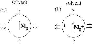
Figure 3: Cartoon of the solvent polarization around a dipolar solute. A higher number of solvent dipoles in the equatorial plane of the solute dipole $\mathbf{M}_{0}$ (a) yields a negative value of the response function $\chi_{0s}$. In panel (b), the addition of equatorial charges to the solute does not alter the solute dipole calculated relative to the center of the sphere, but polarizes equatorial waters in a direction orthogonal to $\mathbf{M}_{0}$. The results is a positive $\chi_{0s}$, as indeed found for all charged proteins here.

We show in Appendix A that the second summand in Eq. (20) is zero when the continuum, $k\rightarrow 0$ limit is taken in the homogeneous solvent response function $\bm{\chi}_{s}(\mathbf{k})$. We will use this limit throughout below since the typical size of the protein $2R$ significantly exceeds the diameter of water. Within this approximation one arrives (see Appendix A) at $\chi_{0s}$ and then at the following connection between the $\chi_{0s}$ and $\chi_{00}$ response functions in terms of the interfacial dipolar susceptibility $\chi_{1}$

$$\chi_{0s}=-\frac{2}{3}\frac{\epsilon_{s}-1}{\epsilon_{s}}\left(1-(4\pi/3)\epsilon_{s}\chi_{1}\right)\chi_{00}.$$ (22)

From this equation and Eq. (10), one additionally have

$$\frac{\chi_{0}^{d}}{\chi_{00}}=\frac{\epsilon_{s}+2}{3\epsilon_{s}}+\frac{8\pi}{9}(\epsilon_{s}-1)\chi_{1}.$$ (23)

If the term in the brackets in Eq. (22) is positive, as is the case in both the Lorentz and Maxwell scenarios, $\chi_{0s}$ is negative. Figure 3a illustrates the physical origin of this result. The solvent polarization is a sum of two compensating contributions. The solvent dipoles at the poles of the solute dipole will predominantly orient parallel to $\mathbf{M}_{0}$, while equatorial solvent dipoles will orient antiparallel to $\mathbf{M}_{0}$. Since there are more equatorial dipoles than there are pole dipoles, $\chi_{0s}<0$ for the overall solvent polarization.

It is instructive to see what are the numerical outputs for $\chi_{0}^{d}$ in the Maxwell and Lorentz scenarios sketched in Fig. 1. In the Lorentz case of $\chi_{1}=0$ one gets

$$\chi_{0}^{d}=\frac{\epsilon_{s}+2}{3\epsilon_{s}}\chi_{00}.$$ (24)

The correction term in front of $\chi_{00}$ is the Lorentz cavity field which indeed appears in polar response when the surface of a cavity cut from the dielectric is not polarized.Frohlich ; Scaife:98

When the Maxwell result [Eq. (15)] for the susceptibility $\chi_{1}$ is used in Eq. (22) one gets

$$\chi_{0}^{d}=\frac{3}{2\epsilon_{s}+1}\chi_{00}.$$ (25)

This correction factor is the well-known cavity field of the theories of dielectrics.Frohlich ; Scaife:98 These arguments stress again (see above) that specifying an algorithm of calculating $\mathbf{M}_{s}$ in terms of $\mathbf{M}_{0}$ leads to a route to formulate a theory of polar response, with the prescription of Figs. 1a and 2 corresponding to Maxwell’s electrostatics.Landau8 ; Frohlich ; Scaife:98

Equations (24) and (25) are special cases of a more general result

$$\frac{\chi_{0}^{d}}{\chi_{00}}=\frac{E_{c}}{E_{0}}$$ (26)

connecting the cavity field inside the solute $E_{c}$ with the ratio of two response functions. The notion “cavity” here implies that this field is produced by the solvent polarized by the external field and does not include any reaction fields of the solute charges. While the two contributions into the overall electric field inside the solute might seem to be hopelessly entangled, they are in fact separable in the frequency domain. The solute and corresponding reaction fields are dynamically frozen at frequencies above the Debye peak of the solute, in most practical cases well below the Debye peak of the water component of the solution. The observation of the dielectric increment of the water’s Debye peak as a function of the solute concentration in the limit of ideal solution provides a direct access to the cavity fieldDMjcp2:11 and, by Eqs. (23) and (26), to the ratio of the two susceptibilities and $\chi_{1}$. The relation of these susceptibilities to dielectrophoresis discussed below is yet another connection to the laboratory experiment.

A significant difference in the solute dipolar response predicted by Lorentz and Maxwell polarization scenarios offers an opportunity to control the interaction of the solute dipole with an external field by changing the distribution of the surface charge. For example, consider the effect of surface charges placed in the equatorial region of the global solute dipole in Fig. 3b. These charges will not change the overall solute dipole calculated relative to the sphere’s center, but will orient solvent dipoles perpendicular to the global dipolar field of the solute and can potentially invert the sign of $\chi_{0s}$. This is indeed what we find in our simulations of charged hydrated proteins.

One can also anticipate some combination of the solute shape and charge distribution that will produce a negative net result for $\chi_{0}$, when negative $\chi_{0s}$ exceeds in magnitude $\chi_{00}$. This outcome, which can be characterized as overscreeningBallenegger:05 of the solute dipole by the hydration layer, would correspond to a dia-electric response of the solute, i.e. its repulsion from the region of a more intense electric field. We find this result in our simulations of the neutral ubiquitin (ubiq) protein.

IV Results of MD Simulations

Equation (22) is a central result of our derivation. It connects the two component of the solute dipolar susceptibility and the interface moment $M_{0}^{\text{ind}}$ to one single property, the dipolar susceptibility of the interface $\chi_{1}$. This susceptibility is a coarse-grained parameter incorporating the effects of both the shape and surface charge distribution of the solute. Since both $\chi_{0s}$ and $\chi_{00}$ are in principle accessible from numerical simulations, Eq. (22) allows us to construct the overall dipolar response of a hydrated solute without additional assumptions on the nature of polarization boundary conditions at the interface.

Four globular proteins, reduced form of cytochrome c (cytC, 100 ns, PBD database 2B4Z), ubiquitin (ubiq, 172 ns, 1UBQ), lysozyme (lys, 153 ns, 3FE0), and reduced form of cytochrome B562 (cytB, 123 ns, 256B) were studied by long, 100–172 ns all-atom Molecular Dynamics (MD) simulations. The overall length of the simulation trajectories was $>0.5$ $\mu$s. All proteins were solvated in large numbers of TIP3P waters to achieve mM protein concentration typically used in experimental solution measurements. The number of waters in the simulation box were $N_{s}=33189$ (cytC), 27918 (ubiq), 27673 (lys), and 33268 (cytB). From these proteins, cytB is the only protein with the overall negative charge $Z$ (Table 1), and it was chosen mostly for that reason.

The importance of long simulations has been recognized in previous attempts to address the dielectric properties of protein solutions, Smith:93 ; Simonson:96 ; Boresch:00 ; Schroder:06 ; Rudas:06 but they had never reached the length and system size reported here. In particular, Steinhauser and co-workers Loffler:97 ; Boresch:00 ; Rudas:06 have pointed to a significant contribution of $\chi_{0s}$ susceptibility to the overall dipolar response of the solution, but could reach only qualitative conclusions from trajectories available to them ($\simeq 13-30$ ns). Many previous attempts to simulate protein solutions had suffered from even shorter trajectories and far smaller simulation boxes. The aim of this round of simulations is to extend previous simulation studies to reliably calculate both $\chi_{00}$ and $\chi_{0s}$ components of the solute dipolar response. We therefore do not approach here the calculation of the overall dielectric response of the protein solution and instead focus on the question of how polar, as probed by $\chi_{0}$, a hydrated protein can be. The details of the simulation protocol can be found in the Supplementary Material (SM)supplJCP and we proceed directly to the results.

Table 1: Dielectric parameters of hydrated proteins from MD simulations.

Protein	$Z$	$R$ (Å)	$\epsilon_{0}$	$\langle M_{0}\rangle$ (D)	$\chi_{0}^{d}$	$\chi_{00}$	$\chi_{0s}$	$\chi_{0}^{\text{int}}\times 10^{3}$	$\chi_{1}/\chi_{1}^{\text{M}}$	$\kappa_{1}$
Lys	$+7$	19.2	62	223	4.9	3.9	1.0	3.7	$-2.8$	0.3
CytC	$+6$	18.7	639	367	51	38	13	3.9	$-3.1$	5.7
Ubiq	$0$	17.8	0.5	244	$-0.04$	0.17	$-0.21$	$-2.3$	$1.78$	0.2
CytB	$-5$	23.5	96	196	7.5	6.1	1.4	3.6	$-2.8$	21.6

IV.1 Static properties

The proteins studied here are similar in their effective size, as calculated from the volume inside the solvent-accessible surface enveloping the molecule.Till:10 The average dipole moments $\langle M_{0}\rangle$ calculated from the protein partial charges and averaged over the trajectories are also close in magnitude and are in basic agreement with dipole moments typically reported by dielectric spectroscopy of protein solutionsTakashima:89 (Table 1). The values of the dipole moments were calculated here relative to the protein center of mass since these dipoles appear in the equations of motion establishing the torque applied to the protein by an external electric field.Rudas:06 While the protein size and the dipole moment appear to be generic for the set of globular proteins studied here, the dipolar susceptibility, i.e. the variance of the protein dipole is quite specific for a given protein. We find a remarkably broad range of dipolar susceptibilities $\chi_{0}$ and the corresponding values of $\epsilon_{0}=1+4\pi\chi_{0}$ among the proteins studied here (Table 1).

The polarity of the protein, as measured by $\chi_{0}$ or $\epsilon_{0}$, does not seem to correlate with either the magnitude or the sign of the overall protein charge. In fact, values of $\epsilon_{0}$ are close for positively charged lys ($Z=+7$) and negatively charged cytB ($Z=-5$). A significant variation in the values of $\epsilon_{0}$ found here (Table 1) seems to originate from differences in surface charge distributions of the proteins and the corresponding polarization of the hydration water.

The cross-correlation susceptibility $\chi_{0s}$ also varies significantly among the proteins, both in magnitude and sign. We find $\chi_{0s}$ positive for the charged proteins. This observation can be explained in terms of the water polarization scenario pictured in Fig. 3b. In contrast, $\chi_{0s}$ is negative for the neutral ubiq, in agreement with the dielectric arguments presented above. However, in contrast to the standard expectations, $\chi_{0}^{d}$ is negative. This outcome implies a dia-electric response or negative dielectrophoresis. The relative error of this claim is 20% (Table 1). This is because $\chi_{0}^{d}$ comes as a small number from subtraction of two relatively large numbers, $\chi_{00}$ and $\chi_{0s}$, and converges very slowly even on the longest trajectory we have run in this study (see the SMsupplJCP ).

The results for the interface susceptibility $\chi_{1}$ are consistent with the results for $\chi_{0s}$ (Table 1). The susceptibility $\chi_{1}$ not only exceeds the Maxwell $\chi_{1}^{\text{M}}$ [Eq. (15)] in magnitude, but has the sign opposite to it. A positive $\chi_{1}$ physically means that the dipole produced by the surface charge density $\sigma_{P}$ (Fig. 2) is oriented along the field and not opposite to the field as the Maxwell scenario would suggest. As for $\chi_{0s}$, the origin of this outcome should be sought along the lines illustrated in Fig. 3b, which shows that different regions of the interface polarization can add constructively or destructively depending on the distribution of the surface charge.

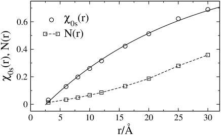
Figure 4: Reduced functions $\chi_{0s}(r)/\chi_{0s}$ (circles) and $N(r)/N_{s}$ (squares) calculated from the layer of water of thickness $r$ surrounding the vdW surface of cytC. Here, $\chi_{0s}$ is calculated for the entire simulation cell containing $N_{s}$ waters. The solid lines is the fit of $\chi_{0s}(r)/\chi_{0s}$ to an exponential function, $1-\exp[-(r-a)/\lambda]$, with $\lambda=24$ Å and $a=2.6$ Å. The dashed line connects the simulation points.

Spatial correlation between the protein and water dipoles are found to be long-ranged. This is illustrated in Fig. 4 where we plot $\chi_{0s}(r)$ and $N(r)$ reduced to their values obtained from the entire simulation box. Function $N(r)$ is a number of waters in a shell of thickness $r$ as measured from the protein van der Waals (vdW) surface; $\chi_{0s}(r)\propto\langle\delta\mathbf{M}_{0}\cdot\delta\mathbf{M}_{s}(r)\rangle$ is the cross-correlation function obtained from the total dipole moment $\mathbf{M}_{s}(r)$ of all waters within the same shell. Although $\chi_{0s}(r)$ clearly goes faster to its saturation limit than the number of waters in the cell, it reaches only half of its cell value for seven water shells around the protein. In fact when $\chi_{0s}(r)/\chi_{0s}$ is fitted to an exponential decay function (solid line in Fig. 4), the corresponding correlation length turns out to be 24 Å.

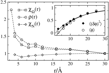
Figure 5: Dependence on the thickness $r$ of the solvation shell of the water number density $\rho(r)=N(r)/\Omega(r)$ and two dielectric susceptibilities, $\chi_{\Omega}(r)$ and $\chi_{N}(r)$ (see the text for the definitions). The inset shows the average potential $\langle\phi(r)\rangle$ at the Fe atom of the heme (open circles) and its variance $\langle(\delta\phi(r))^{2}\rangle$ (closed diamonds). The dashed lines in the main panel connect the points and the solid lines in the inset are fits of the simulation data to the function $1-\exp[-(r-a)/\lambda]$, with $\lambda=12$ Å and 13 Å for the potential and its variance, respectively. The calculations have been performed for cytC. All results in the main panel are normalized to their corresponding values at $r=30$ Å, while the data in the inset are normalized to the results obtained for the entire simulation box.

The nearly disappearance of the cross-correlation between the protein and shell dipoles at the shell thickness $r$ approaching the limit of one hydration layer implies that waters in the first solvation shell do not much correlate with the overall protein dipole and are more driven by the local fields and vdW forces of the surface groups. It is only more distant layers that correlate more extensively with the global electrostatics of the solution. This picture contrasts with a more localized density response of the interface shown in Fig. 5. The density profile $\rho(r)=N(r)/\Omega(r)$ ($\Omega(r)$ is the shell volume) peaks at the interface, indicating wetting of the protein surface by water, and then decays to approximately the bulk density within $\sim 3$ solvation layers ($\simeq 10$ Å).

We also show in Fig. 5 the dielectric susceptibility of the surface waters determined by correlating the dipole moment of the shell $\mathbf{M}_{s}(r)$ with the total dipole moment of water $\mathbf{M}_{s}$.DMcpl:11 We define two susceptibilities, normalized to the number of shell waters, $\chi_{N}(r)\propto N(r)^{-1}\langle\delta\mathbf{M}_{s}(r)\cdot\delta\mathbf{M}_{s}\rangle$, and the susceptibility normalized to the shell volume, $\chi_{\Omega}(r)\propto\Omega(r)^{-1}\langle\delta\mathbf{M}_{s}(r)\cdot\delta\mathbf{M}_{s}\rangle$. While the former is almost flat, showing virtually no variation of polarity near the interface, susceptibility $\chi_{\Omega}(r)$ shows about 30% increase related to the corresponding increase of the interfacial density. This polarity increase is below the increment observed at the interface of a non-polar solute with water,DMcpl:11 reflecting the topological and chemical heterogeneityChengRossky:98 ; Giovambattista:08 of the protein surface.

Figure 5 suggests that interfacial properties scaling as interfacial density will mostly decay to their bulk values within $\sim 3$ hydration layers. However, this rule should not be blindly extended to other observables. In particular, the electrostatic response of the interface is only indirectly affected by density and in principle can have a different range of convergence. This is shown in the inset in Fig. 5 which presents the accumulation of the average and variance of the electrostatic potential $\phi(r)$ produced by waters from the $r$-shell at the Fe atom of the heme. The accumulation of both the average and the variance are much slower than the decay of the interfacial density and are in fact comparable in range to the accumulation of the cross-correlation $\chi_{0s}(r)$ shown in Fig. 4. Specifically, when these data are fitted to exponential decay functions, similarly to what has been done for $\chi_{0s}(r)$, one gets the correlation lengths of 12–13 Å.

IV.2 Dynamical properties

The long range of the dipolar protein-water correlation appearing in susceptibility $\chi_{0s}$ will be masked in $\chi_{0}^{d}$ by a larger in magnitude self protein component $\chi_{00}$. The two susceptibilities exhibit, however, different dynamics, as is shown in Fig. 6 for their loss functions. These are calculated from the time correlation function

$$S_{0}(t)=\left[\langle\delta\mathbf{M}_{0}\cdot\delta\mathbf{M}\rangle\right]^{-1}\langle\delta\mathbf{M}_{0}(t)\cdot\delta\mathbf{M}(0)\rangle$$ (27)

and the corresponding self and cross correlation functions

$$S_{0a}(t)=\left[\langle\delta\mathbf{M}_{0}\cdot\delta\mathbf{M}_{a}\rangle\right]^{-1}\langle\delta\mathbf{M}_{0}(t)\cdot\delta\mathbf{M}_{a}(0)\rangle,$$ (28)

where $a=0,s$. In the case of lys, there is about a factor of four difference between the main Debye peaks of $\chi_{00}(\omega)$ ($\simeq 14$ ns) and $\chi_{0s}(\omega)$ ($\simeq 3.5$ ns). There is therefore a frequency window in which the two components of the overall dipolar susceptibility can be separated. It is also worth mentioning here that two relaxation times identified here for $\chi_{0s}(\omega)$, 3.5 ns and 14 ps (lys), bracket the typical dielectric $\delta$-relaxation band observed between protein and water frequency peaks in dielectric loss functions of protein solutions.Oleinikova:04 The solute-solvent dipolar cross-correlations are considered as a plausible cause of the $\delta$-dispersion.Boresch:00 ; Schroder:06 ; Rudas:06

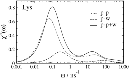
Figure 6: Normalized loss function ($\int_{0}^{\infty}\chi^{\prime\prime}(\omega)d\omega/(\pi\omega)=1$) obtained from the time cross-correlation function $S_{0}(t)$ (Eq. (27), solid line). The self protein-protein (dash-dotted line, p-p) and cross protein-water (dashed line, p-w) loss functions are obtained from the corresponding time correlation functions in Eq. (28). Their relative weights reflect contributions of $\chi_{00}$ and $\chi_{0s}$ to $\chi_{0}^{d}$. The calculations were done for hydrated lys.

Both electrostatic and binding properties of surface waters are highly heterogeneous, but this reality is differently reflected by the observables. The dynamics of the protein dipole moment are essentially single-exponential, decaying on the characteristic time of 4–14 ns of protein tumbling. The dynamics of the dipole moment of the first hydration layer are also fairly generic. The correlation functions decay much faster (see the SMsupplJCP ), but still contain a 10–20% slow component with the relaxation time close to that of the protein dipole. This slow component can be assigned to waters strongly attached to the protein surface.Bone:85

In contrast to the generic dynamics of the protein and first-shell dipoles, the population dynamics of the first layer are more specific. The self-correlation functions $S_{N}(t)$ of the number of first-shell waters $N_{1}(t)$ follows the rotational dynamics of $\mathbf{M}_{0}(t)$ for cytC and cytB (Fig. 7). It appears that waters in the first layer of these two proteins are strongly bound to the protein surface positionally, but can rotate relatively freely, resulting in fast relaxation of the first-shell dipole moment. On the contrary, waters are weakly bound to the surface of lys and ubiq, with significantly faster decays of their populations (Fig. 7).

The binding affinity of the first-shell waters is, however, heterogeneous. This is seen particularly clear for ubiq. Its initial relaxation is two-exponential, with relaxation times of 0.2 ps (58%) and 39 ps (30%). This initial fast decay is followed, however, by a plateau indicating that about 12% of first-shell waters do not leave the protein surface on the simulation time-scale. A similar long-time component, contributing to about 17% of the correlation function, was found for cytB (see the SMsupplJCP ).

In addition to the differences in the first-shell population dynamics seen for the two pairs of proteins, the first-shell compressibilities $\langle(\delta N_{1})^{2}\rangle/\langle N_{1}\rangle$ are quite different for them as well (last column in Table 1). The compressibilities of first shells of lys and ubiq are similar to those found for water shells around rigid non-polar solutes,MittalHummer:08 ; DMcpl:11 while they are much higher for the two cytochromes. It is not yet clear how this observation relates to the corresponding differences in the population dynamics.

To connect these observations to our electrostatic problem, it seems clear that different observables variably report on the protein-water interfacial structure. The dipolar response of a protein is particularly sensitive to the distribution of the surface charge and might potentially be considered as a marker of a given protein. High variability of $\epsilon_{0}$ among the proteins offers a potential for applications to protein detection and separation in solution.

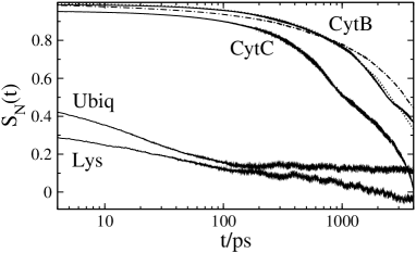
Figure 7: Normalized time self-correlation functions of the number of waters in the first hydration shell $S_{N}(t)$. The data are obtained from MD simulations; multi-exponential fits of the correlation functions are given in the SM.supplJCP The dash-dotted and dotted lines indicate the self correlation functions $S_{00}(t)$ [Eq. (28)] of the protein dipole for cytB and cytC, respectively.

V Dielectrophoresis of protein solutions

Inhomogeneous external electric field exerts a force on the solute dipole.JonesBook:95 ; HughesBook:03 This is given by the expression

$$\mathbf{F}_{0}=\frac{3\Omega_{0}}{8\pi\epsilon_{s}}K\nabla E_{0}^{2},$$ (29)

where $K=(4\pi/3)\epsilon_{s}(\chi_{0}^{d}+\chi_{0}^{\text{int}})$ is the dielectrophoresis constant. The solute is dragged toward a stronger field if $K>0$ (positive dielectrophoresis) or toward a weaker field if $K<0$ (negative dielectrophoresis).

We will use Eq. (22) to remove dipolar cross-correlations and recast $K$ in terms of susceptibilities $\chi_{00}$ and $\chi_{1}$. One gets

$$K=\frac{\epsilon_{s}+2}{3}y_{0}+\frac{4\pi}{3}\epsilon_{s}\chi_{1}\left[1+\frac{2}{3}(\epsilon_{s}-1)y_{0}\right],$$ (30)

where the dipolar density of the solute $y_{0}=y_{e}+(4\pi/3)\chi_{00}$ is introduced in analogy to the dipolar density of a polar liquidScaife:98 ; SPH:81 $y=(4\pi/9)\beta\rho m^{2}$; here, $m$ and $\rho$ are the dipole moment and number density of a liquid. We have included the component $y_{e}$ into $y_{0}$ originating from electronic polarizability of the solute, which has not been considered so far, but needs to be included in high-frequency calculations. This component is additive to the one arising from the permanent dipoleSPH:81 and can be connected to the measurable refractive index of the protein $n_{0}$ by the Clausius-Mossotti equation, $y_{e}=(n_{0}^{2}-1)/(n_{0}^{2}+2)$.

The two limiting, Lorentz and Maxwell, scenarios are worth emphasizing here. In the Lorentz scenario, $\chi_{1}=0$ and one gets

$$K_{\text{L}}=\frac{\epsilon_{s}+2}{3}y_{0}.$$ (31)

The factor in front of $y_{0}$ can be recognized as the Lorentz cavity field correction.Scaife:98 Further, this equation allows only positive dielectrophoresis.

In the Maxwell scenario, $\chi_{1}=\chi_{1}^{\text{M}}$ [Eq. (15)], one gets

$$K_{\text{M}}=\frac{3\epsilon_{s}}{2\epsilon_{s}+1}y_{0}-\frac{\epsilon_{s}-1}{2\epsilon_{s}+1}.$$ (32)

Now, the factor in front of $y_{0}$ is the standard cavity field of traditional dielectric theories.Scaife:98 Negative dielectrophoresis is now allowed when the threshold value $y_{0}^{*}=(\epsilon_{s}-1)/(3\epsilon_{s})$ is reached.

The standard analysis of dielectrophoresis of non-polar colloidal suspensions HughesBook:03 neglects the dipole moment of the solute, assuming $y_{0}\simeq 0$ in Eq. (32). In addition, when a dielectric constant $\epsilon_{0}$ can be assigned to the material of the colloidal particle, $\epsilon_{s}$ in the second summand of Eq. (32) is replaced by $\epsilon_{s}/\epsilon_{0}$, according to the standard rules for the electrostatics of dielectric interfaces.Landau8 The result is the traditional constant of dielectrophoresis commonly used in the analysis of colloidal suspensionsWangPethig:93

$$K=\frac{\epsilon_{0}-\epsilon_{s}}{\epsilon_{0}+2\epsilon_{s}}.$$ (33)

This approximation is not applicable to protein solutions and we will instead explicitly consider the dipolar response of the protein, with susceptibilities $\chi_{00}$ and $\chi_{1}$ in Eq. (30) from MD simulations.

Dielectrophoresis measurements are typically performed with oscillatory external fields. The static properties considered so far need to be replaced with frequency-dependent response function according to the standard rules of handling time correlation functions.Hansen:03 While the frequency-dependent dielectric constant of water is well defined and tabulated from laboratory measurements, more care is required to define the frequency dependent susceptibility $\chi_{1}(\omega)$ and $y_{0}(\omega)$.

The standard rules of connecting the response functions to time correlation functions sugest the following form for the frequency-dependent response functions of the solute dipole DMpre:10

$$\chi_{0a}(\omega)=\chi_{0a}\left[1-i\omega\tilde{S}_{0a}(-\omega)\right],$$ (34)

where $a=0,s$ and $\tilde{S}_{0a}(\omega)$ is the Fourier-Laplace transform of the corresponding time correlation functions in Eq. (28). These two relations, with $\tilde{S}_{0a}(\omega)$ obtained from MD simulations, can be used in Eq. (22) to find $\chi_{1}(\omega)$. In doing that, one needs to replace $\epsilon_{s}$ with the frequency-dependent, complex-valued dielectric constant of water $\epsilon_{s}(\omega)$. Once this is done, one can employ Eq. (30) with the frequency-dependent susceptibilities and $\mathrm{Re}[K(\omega)]$ in Eq. (29) to calculate the force.WangPethig:93 ; HughesBook:03 The effect of the electrolyte can be included into the water dielectric constant $\epsilon_{s}(\omega)=\epsilon_{D}(\omega)+\sigma_{i}/(i\omega)$ through the ionic conductivity of the solution $\sigma_{i}$, in addition to the Debye dielectric constant $\epsilon_{D}(\omega)=\epsilon_{D}^{\prime}(\omega)+i\epsilon_{D}^{\prime\prime}(\omega)$ for the dielectric response of pure water.

The results of calculations of $\mathrm{Re}[K(\omega)]$ for cytB and lys are shown in Fig. 8. The dynamics of the protein’s dipole, $\chi_{00}(\omega)$ and $\chi_{0s}(\omega)$ are taken directly from MD simulations (see the SMsupplJCP for the fits of the relaxation functions and the list of the relaxation times). The frequency-dependent dielectric constant of water $\epsilon_{D}(\omega)$ is taken from Ref. Yada:09, and $n_{0}=1.47$ is assigned to the protein. The electrolyte conductivity in the range $\sigma_{i}\simeq 1-100$ mSm^-1 typically employed in the laboratory measurements HughesBook:03 does not affect the outcome of the calculations.

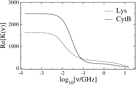
Figure 8: $\mathrm{Re}[K(\nu)]$, $\omega=2\pi\nu$ from Eq. (30) with the frequency-dependent response functions in Eq. (34) from MD simulations and $\epsilon_{D}(\omega)$ of water from Ref. Yada:09, ; the refractive index of the protein $n_{0}=1.47$.

The main result of these calculations is a dominance of $y_{0}(\omega)$, arising from the protein permanent dipole, in the overall dielectrophoresis response. This result holds for all charged proteins studied here. In contrast, even static dielectrophoresis constant is negative for ubiq, suggesting negative dielectrophoresis in the entire frequency range. Numerical difficulties in obtaining $S_{0s}(t)$ for ubiq have prevented us from presenting $K(\omega)$ for this protein.

VI THz absorption of protein solutions

Positive $\chi_{1}$, instead of the negative values in both the Lorentz and Maxwell scenarios, alter the theory predictions concerning the absorption of THz radiation by protein solutions. We have recently suggested a model,DMpre:10 based on the formalism of response functions discussed in Sec. III, to address this problem. The study was motivated by experimental reports of the positive slope of the absorbance increment with an increasing concentration of the protein in solution, following by a non-linear downward turn of the concentration dependenceEbbinghaus:07 ; Born:09 (inset in Fig. 9). Such a trend, recorded in the 1–3 THz frequency range, contradicts the traditional view that adding a protein, less polar than water, should lower the solution polarity and the corresponding radiation absorbance. Indeed, the model calculations in Ref. DMpre:10, could not account for the observations without demanding a significant increase of the effective dipole of the protein-water interface. That development was, however, based on the Maxwell scenario for the interface susceptibility and thus negative interface dipole. Since the present formalism goes beyond the Maxwell picture and the numerical results allow a positive interface dipole, this problem needs to be revisited.

We are looking at the absorbance of the electromagnetic radiationLandau8

$$\alpha(\omega)=\frac{4\pi\omega}{c}\ \frac{\chi^{T^{\prime\prime}}(\omega)}{\sqrt{1+4\pi\chi^{T^{\prime}}(\omega)}},$$ (35)

where $c$ is the speed of light and the superscript “T” emphasizes that we are considering the susceptibility of the solution $\chi(\omega)$ in the direction of the electric field perpendicular (transversal) to the direction of light propagation determined by the wave-vector. The property reported experimentally is the relative increment $\Delta\alpha(\omega)/\alpha_{s}(\omega)=\alpha_{\text{mix}}(\omega)/\alpha_{s}(\omega)-1$ of the solution (mixture) absorbance over the absorbance of the homogeneous liquid $\alpha_{s}(\omega)$.

The derivation of the solution absorbance directly follows from the generalized response function in Eq. (11). The derivation steps follow Ref. DMpre:10, and are briefly summarized in Appendix B. One gets the following result for the relative susceptibility increment

$$\begin{split}\Delta&\chi^{T}(\omega)/\chi^{T}_{s}(\omega)=-\eta_{0}\left[1-\frac{4\pi}{3}\epsilon_{s}(\omega)\chi_{1}(\omega)\right]\\ &+y_{0}(\omega)\eta_{0}\left[\frac{\epsilon_{s}(\omega)+2}{\epsilon_{s}(\omega)-1}+\frac{8\pi}{3}\chi_{1}(\omega)\epsilon_{s}(\omega)I_{0}(\eta_{0},R)\right],\end{split}$$ (36)

where $\Delta\chi^{T}(\omega)=\chi_{\text{mix}}^{T}(\omega)-\chi^{T}_{s}(\omega)$ and $\chi_{s}^{T}(\omega)=(\epsilon_{s}(\omega)-1)/(4\pi)$. Further, $\eta_{0}$ is the volume fraction of the solutes and $I_{0}(\eta_{0},R)$ represents the mutual polarization of the solutes by their permanent dipoles aligned by the field of radiation, a non-ideal solution effect. It is given by Eq. (57) in Appendix B and has been tabulated as a function of $\eta_{0}$ and $R$ in Ref. DMpre:10, assuming hard-sphere structure factor for the solutes in solution. This latter approximation has been used in the calculations presented in Fig. 9.

All the parameters in Eq. (36) are defined in our calculations of the dielectrophoresis response and are directly applied to the calculations shown in Fig. 9 for cytB. The solid line shows $\Delta\alpha(\omega)/\alpha_{s}(\omega)$ calculated at 2.25 THz of radiation used in the experiment.Ebbinghaus:07 The result is an obviously positive slope of the absorption increment, which arises from both the interface and permanent dipoles re-enforcing each other. In contrast, both Lorentz and Maxwell scenarios suggest a negative slope (dashed line in Fig. 9).

The non-linear dependence on the solute volume fraction present in $I_{0}(R,\eta_{0})$ in Eq. (36) turns out to be insufficient to bend the concentration dependence downward (inset in Fig. 9). Several possible long-range effects are still missing from our analysis. The structure factor of solvated proteins is estimated from its hard-sphere limit and can be modified by long-ranged interactions. In addition, correlation between proteins’ dipole moments, represented by the Kirkwood factor, has not been included in the present calculation.DMpre:10 We, however, want discuss yet another possibility related to the long decay of the solute-solvent dipolar correlations shown in Fig. 4.

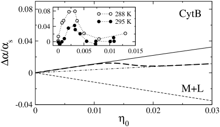
Figure 9: Absorbance increment calculated at the frequency of 2.25 THz vs the molar fraction $\eta_{0}$ of cytB in water. The calculation with $\chi_{1}(\omega)$ from MD simulations (solid line) is compared to $\chi_{1}(\omega)$ from either Maxwell or Lorentz scenarios (dashed line, labeled “M+L”) which give very close results in this frequency range. The dash-dotted line is the calculation performed with the restriction $(4\pi/3)\epsilon_{s}(\omega)\chi_{1}(\omega)=1$ corresponding to zero $\chi_{0s}$ in Eq. (22). The bold dashed line is arbitrary drawn to illustrate a crossover between two linear slopes when proteins in solution start to affect each other and prevent full convergence of $\chi_{0s}(r)$ characterized by a long correlation length of $\simeq 2.4$ nm [Fig. 4]. The inset shows experimental data reported in Ref. Ebbinghaus:07, for a five-helix bundle protein $\lambda^{*}_{6-85}$ at two temperatures indicated in the plot. The dotted lines in the inset connect the points.

The correlation length of $\lambda\simeq 2.4$ nm found in Fig. 4 suggests that susceptibility $\chi_{0s}$ becomes affected when proteins in solution come closer than $2\lambda$, which roughly corresponds to the position of the peak in the experimental concentration dependence in the inset of Fig. 9. If mutual effect of the proteins in solution does not allow $\chi_{0s}$ to saturate, it implies that, according to Eq. (22), $\chi_{1}$ should change with the concentration and approach the limit $(4\pi/3)\epsilon_{s}(\omega)\chi_{1}(\omega)\simeq 1$. This limit for the absorbance is shown by the dash-dotted line in Fig. 9. The overall concentration dependence is expected to exhibit a crossover from one linear slope to another in the concentration range where proteins start to affect each other, as is schematically shown by the bold dashed line in Fig. 9. The experiment shows a qualitatively similar crossover behavior. Further, no cross-over of the concentration dependence of the absorption coefficient was found for solutions of aminoacids.Niehues:2011fk This observation suggests a much shorter length-scale of dipolar cross-correlations for hydrated aminoacids compared to proteins. The reason might be related to a more homogeneous structure of waters around aminoacids and thus a higher contribution of the first hydration layer to $\chi_{0s}$, which is almost absent for proteins (Fig. 4).

A brief comment on the experimental temperature dependence of the absorption shown in the inset of Fig. 9 is relevant here. The permanent dipole susceptibility $\chi_{00}$ is proportional to $\beta$. The slope of the absorbance with concentration is therefore expected to increase with lowering temperature, as is indeed qualitatively observed.

These calculations and qualitative comparisons with experiment suggest that most of the polar response of the protein charges is frozen on the time-scale of THz radiation, which therefore allows one to probe the polarization of the protein-water interface projected on the dipole $M_{0}^{\text{int}}$. This interface polarization is distinctly different from the Lorentz-Maxwell scenario and this fact is reflected in the positive slope of the absorbance with increasing concentration.

VII Summary

In conclusion, we have utilized long simulation trajectories and large system sizes to systematically study the dipolar susceptibility [Eq. (7)] of hydrated proteins. This property exhibits large variation among the proteins, suggesting its possible use as a “marker” of a protein in solution. The large variance in the protein susceptibility also opens the door to their detection and separation in solution, in particular by dielectrophoresis of the protein solutions.

The permanent dipole susceptibility is a combination of the variance of the intrinsic protein dipole and a cross-correlation between the protein and water dipoles. The cross-correlation component is found to be negative for uncharged ubiq, but is positive for the charged proteins. It is also long-ranged, decaying into the bulk on the correlation length of about 2 nm. A similar, but somewhat smaller, decay length is found for the electrostatic potential produced by the hydration water inside the protein.

Dipolar solute-water cross-correlations are significant and cannot be neglected. In the case of ubiq the self and cross correlation components nearly cancel each other, but produce a negative overall susceptibility. This protein therefore demonstrates negative dielectrophoresis and, correspondingly, a dia-electric dipolar response.

Thermodynamic stability prohibits dia-electric response ($\epsilon_{s}<1$) for bulk dielectrics.Landau8 This limitation does not apply to a finite-length polar response,Dolgov:81 and in fact the wave-vector dependent dielectric constant $\epsilon_{s}(k)$ is negative in a certain range of $k$-values for most polar liquids.Raineri:99 Thermodynamic arguments also do not rule out a dia-electric response of solutes in solution. Negative dielectrophoresis is in fact fairly common for colloidal suspensions.HughesBook:03 Nevertheless, this is the first report of negative dielectrophoresis of proteins by numerical simulations.

An important question posed by the present study and requiring further investigation is whether negative values of $\chi_{0}$ found here for ubiq are general for neutral proteins. If the answer to this question is affirmative, dielectrophoresis of hydrated proteins is expected to be sensitive to the buffer pH (as indeed has been reported HughesBook:03 ). In addition, negative dielectrophoresis, and thus dia-electric response, should be common when the buffer pH approaches protein’s isoelectric point. Future simulations and laboratory measurements are required to shed more light on this intriguing perspective. In terms of physiological conditions of protein activity, this possibility would imply a range of pH values in which a protein is nearly insensitive to significant gradients of local electric fields, i.e., “invisible” to local fields.

The interface polarization is a small portion of the static or low-frequency dipolar response, but gains in importance at high frequencies, above the protein Debye peak representing its rotation in solution. In this frequency range, the polar response of the protein charges is dynamically arrested and the response of much faster interfacial waters starts to show up. Here, different dielectric scenarios (such as Lorentz or Maxwell recipes) predict distinctly different outputs. Numerical simulations presented here show a broad range of possibilities, beyond those emphasized by these two electrostatic limits, depending on the distribution of the protein surface charge. These different outcomes are reflected by the THz absorbance of the protein solution. In particular, the sign of the slope of the THz absorbance vs the protein concentration reports on whether the interface dipole is oriented along the polarizing field or opposite to it. A parallel orientation corresponds to a positive slope, whereas an anti-parallel orientation (such as in the Maxwell scenario) yields a negative slope. The measurements of the THz absorbance give therefore a direct access to the polarization pattern of the protein-water interface.

Appendix A Derivation of Eq. (22)

The function $\bm{\chi}(\mathbf{k}_{1},\mathbf{k}_{2})$, first calculated in Refs. DMjcp1:04, and DMjcp2:04, , describes the response of a polar liquid outside a void. The latter is defined by the step function $\tilde{\theta}_{0}(\mathbf{k})$ [Eq. (21)]. This function and its conjugate $\tilde{\theta}=\tilde{1}-\tilde{\theta}_{0}$, $\tilde{1}(\mathbf{k}_{1},\mathbf{k}_{2})=(2\pi)^{3}\delta(\mathbf{k}_{1}-\mathbf{k}_{2})$ together form a set of orthogonal functions projecting the polar response and corresponding electric fields inside and outside the solute. They obey the following orthogonality and multiplication rules: $\tilde{\theta}*\tilde{\theta}_{0}=0$, $\tilde{\theta}*\tilde{\theta}=\tilde{\theta}$, $\tilde{\theta}_{0}*\tilde{\theta}_{0}=\tilde{\theta}_{0}$, where, as above, asterisks refers to the $\mathbf{k}$-space convolution.

The inhomogeneous dipolar response function can then be written as follows

$$\bm{\chi}=\bm{\chi}_{s}-\alpha\bm{\chi}_{s}*\tilde{\theta}_{0}*\mathbf{G}^{-1}*\tilde{\theta}_{0}*\bm{\chi}_{s}.$$ (37)

Here, $\bm{\chi}_{s}(\mathbf{k}_{1},\mathbf{k}_{2})=\bm{\chi}_{s}(\mathbf{k}_{1})\tilde{1}(\mathbf{k}_{1},\mathbf{k}_{2})$ and $\mathbf{G}=\tilde{\theta}_{0}*\bm{\chi}_{s}*\tilde{\theta}_{0}$, which in terms of explicit wave-vectors implies

$$\mathbf{G}(\mathbf{k}_{1},\mathbf{k}_{2})=\tilde{\theta}_{0}(\mathbf{k}_{1}-\mathbf{k}^{\prime})*\bm{\chi}_{s}(\mathbf{k}^{\prime},\mathbf{k}^{\prime\prime})*\tilde{\theta}_{0}(\mathbf{k}^{\prime\prime},\mathbf{k}_{2}).$$ (38)

Equation (37) with $\alpha=1$ presents an exact solution of the problem of dipolar response of a polar liquid interfacing a spherical void.DMjcp1:04 ; DMjcp2:04 It does not, however, anticipate the formation of the specific orientational structure at the interface characteristic of liquid water.Lee:84 ; Sokhan:97 ; Bratko:09 ; Rossky:10 Therefore, $\alpha=\chi_{1}/\chi_{1}^{\text{M}}\neq 1$ is introduced in Eq. (37) to account for possible deviations from the Maxwell scenario of the surface polarization.

From the definition of the response function, the projection of the polarization inside the solute is

$$\tilde{\theta}_{0}*\mathbf{\tilde{P}}=(1-\alpha)\tilde{\theta}_{0}*\bm{\chi}_{s}*\mathbf{\tilde{E}}_{0}.$$ (39)

The polarization projection is of course zero in case of $\alpha=1$ since this is how the response function was constructed.DMjcp1:04 A modification of the inhomogeneous response by $\alpha\neq 1$ in the second term in Eq. (37) is physically equivalent to creating a non-zero dipole associated with the solute. In case of a uniform external field $\mathbf{\tilde{E}}_{0}(\mathbf{k})=\delta_{\mathbf{0},\mathbf{k}}\mathbf{\hat{z}}E_{0}$ this dipole becomes

$$M_{0z}=\mathbf{\hat{z}}\cdot\tilde{\theta}_{0}(-\mathbf{k})*\mathbf{\tilde{P}}(\mathbf{k})=(1-\alpha)\chi_{s}^{L}(0)\Omega_{0}E_{0}.$$ (40)

When the electric field is produced by the solute dipole [Eq. (18)], this field can be written as the projection of the dipolar field outside the solute excluded volume $\mathbf{\tilde{E}}_{0}=\tilde{\theta}*\mathbf{\tilde{E}}_{d}$. Here, $\mathbf{\tilde{E}}_{d}$ is the Fourier-space electric field of a point dipole, without the space cutoff equating the field to zero inside the solute and responsible for the appearance of the spherical Bessel function in Eq. (19). With this representation one gets from Eq. (39)

$$\tilde{\theta}_{0}*\mathbf{\tilde{P}}=(1-\alpha)\tilde{\theta}_{0}*\bm{\chi}_{s}*\tilde{\theta}*\mathbf{\tilde{E}}_{d}.$$ (41)

If $\bm{\chi}_{s}(\mathbf{k})$ here is replaced with its continuum limit $\bm{\chi}_{s}(0)$, the integral becomes identically zero because of the orthogonality of $\tilde{\theta}_{0}$ and $\tilde{\theta}$. The result is $\mathbf{M}_{s}=\mathbf{\tilde{P}}(0)$ in Eq. (20).

If we now choose the direction of $z$-axis along $\mathbf{M}_{0}$ and take the projection of the solute dipole on $\mathbf{\hat{z}}$, we get

$$M_{s,z}/M_{0}=\mathbf{\hat{z}}\cdot\bm{\chi}(0,\mathbf{k})*\mathbf{\tilde{T}}(\mathbf{k})\cdot\mathbf{\hat{z}}.$$ (42)

A note on how to correctly take the $k\rightarrow 0$ limit in the $\mathbf{k}$-space tensor functions is appropriate here. Since both $\mathbf{\hat{z}}$ and $\mathbf{\hat{k}}$ impose axial symmetry on the liquid, which is isotropic in the direct space, one has to take $\mathbf{\hat{k}}$ parallel to $\mathbf{\hat{z}}$ when taking the $k\rightarrow 0$ limit to avoid imposing a bi-axial symmetry. In this prescription, $\tilde{T}_{zz}(0)=-(8\pi/3)$ and one gets for the homogeneous component of $\bm{\chi}(0,\mathbf{k})$ (first summand in Eq. (37))

$$\mathbf{\hat{z}}\cdot\bm{\chi}_{s}(0)\cdot\mathbf{\tilde{T}}(0)\cdot\mathbf{\hat{z}}=-\frac{2(\epsilon_{s}-1)}{3\epsilon_{s}}.$$ (43)

Similarly, one can write down the inhomogeneous component of the polar response from Eq. (11) as

$$\begin{split}(\chi_{1}^{\text{M}})^{-1}\mathbf{\hat{z}}\cdot&\bm{\chi}_{0}(0,\mathbf{k})*\mathbf{\tilde{T}}(\mathbf{k})\cdot\mathbf{\hat{z}}=\\ &\frac{6\Omega_{0}}{\pi R^{2}\chi_{s}^{L}(0)}\int_{0}^{\infty}dkj_{1}(kR)^{2}\langle\mathbf{\hat{z}}\cdot\bm{\chi}_{s}(\mathbf{k})\cdot\mathbf{\tilde{D}}\cdot\mathbf{\hat{z}}\rangle_{\omega_{k}},\end{split}$$ (44)

where $\langle\dots\rangle_{\omega_{k}}$ refers to the average over the solid angles of the unit vector $\mathbf{\hat{k}}$ and

$$\tilde{\theta}_{0}(k)/\Omega_{0}=3\frac{j_{1}(kR)}{kR}$$ (45)

has been used. Using the relations $\langle\mathbf{\hat{z}}\cdot\mathbf{J}^{L}\cdot\mathbf{\hat{z}}\rangle_{\omega_{k}}=(1/3)$ and $\langle\mathbf{\hat{z}}\cdot\mathbf{J}^{T}\cdot\mathbf{\hat{z}}\rangle_{\omega_{k}}=(2/3)$ one gets in the continuum limit $k\rightarrow 0$ for the response function $\bm{\chi}_{s}(\mathbf{k})$

$$(\chi_{1}^{\text{M}})^{-1}\mathbf{\hat{z}}\cdot\bm{\chi}_{0}(0,\mathbf{k})*\mathbf{\tilde{T}}(\mathbf{k})\cdot\mathbf{\hat{z}}=-(8\pi/9)(\epsilon_{s}-1),$$ (46)

where

$$(6R/\pi)\int_{0}^{\infty}j_{1}(kR)^{2}dk=1$$ (47)

and Eqs. (12) for the $k=0$ values of $\chi_{s}^{L,T}(0)$ have been used. Combining Eqs. (43) and (46), one arrives at Eq. (22).

A similar procedure can be applied to calculate the dipole moment of the solvent in uniform external field $\mathbf{\tilde{E}}_{0}(\mathbf{k})=\delta_{\mathbf{0},\mathbf{k}}\mathbf{\hat{z}}E_{0}$. The dipole moment in this case is

$$M_{s,z}=\mathbf{\hat{z}}\cdot\tilde{\theta}(-\mathbf{k}^{\prime})*\bm{\chi}(\mathbf{k}^{\prime},\mathbf{k})*\mathbf{\tilde{E}}_{0}(\mathbf{k}).$$ (48)

According to the preceding arguments, $\tilde{\theta}*\bm{\chi}=\bm{\chi}-(1-\alpha)\tilde{\theta}_{0}*\bm{\chi}_{s}$. From this relation one gets

$$M_{s,z}=M_{\text{liq}}+M_{0z}^{c}=M_{\text{liq}}-M_{0z}+M_{0z}^{\text{int}},$$ (49)

where $M_{0z}$ is given by Eq. (40) and $M_{\text{liq}}$ is the dipole induced by $E_{0}$ in a homogeneous liquid without the solute. Further, $M_{0z}^{c}$ in Eq. (49) is the “cavity dipole” associated with inserting the excluded solute volume into the polarized liquid. It is given as

$$M_{0z}^{c}/(\Omega_{0}E_{0})=\chi_{1}-\chi_{s}^{L}(0)\left(1-\chi_{1}/\chi_{1}^{\text{M}}\right).$$ (50)

Equations (49) and (50) yield Eq. (2) for the overall solution dipole.

Appendix B Derivation of Eq. (36)

We want to calculate the dipole moment $M^{T}(\omega)$ of the solution induced by a polarized electromagnetic wave propagating along the $z$-axis of the laboratory frame and having the electric field vector along the $x$-axis of the same frame. The wave-vector is therefore along $\mathbf{\hat{z}}$ and the response is transversal. The susceptibility in Eq. (35) becomes

$$\chi^{T}(\omega)=M^{T}(\omega)/(VE_{0}).$$ (51)

The formalism of response functionsDMjcp1:04 ; DMpre:10 described in Appendix A gives the following prescription for the calculation of the dipole moment of the solution projected on $\mathbf{\hat{x}}$

$$M^{T}=\chi_{00}\Omega_{0}N_{0}E_{0}+\mathbf{\hat{x}}\cdot\tilde{\theta}(\mathbf{k})*\bm{\chi}(\mathbf{k},\mathbf{k}^{\prime})*\mathbf{\tilde{E}}_{0}(\mathbf{k}^{\prime}).$$ (52)

The first term in this equation (dependencies on frequency are omitted for brevity) is the direct polarization of the permanent dipoles of $N_{0}$ solutes in the mixture and the second term is the polarization of the solvent.

The formalism of Appendix A is now extended to an ensemble of solutes. This extension is straightforward if polarization fields of the liquid around different solutes are uncorrelated.DMpre:10 From Eqs. (11) and (37) one gets

$$\bm{\chi}(\mathbf{k}_{1},\mathbf{k}_{2})=\bm{\chi}_{s}(\mathbf{k}_{1})\delta_{\mathbf{k}_{1},\mathbf{k}_{2}}-\alpha\sum_{i}\bm{\chi}_{0}(\mathbf{k}_{1},\mathbf{k}_{2})e^{i\mathbf{k}_{2}\cdot\mathbf{r}_{i}},$$ (53)

where the sum runs over the $N_{0}$ solutes in the solution. In addition, the source of the electric field now includes the homogeneous external field and the field of all dipolar solutes polarized by it

$$\mathbf{\tilde{E}}_{0}(\mathbf{k})=E_{0}\delta_{\mathbf{0},\mathbf{k}}\mathbf{\hat{x}}+\chi_{00}\Omega_{0}E_{0}\sum_{i}\mathbf{\tilde{T}}(\mathbf{k})\cdot\mathbf{\hat{x}}e^{-i\mathbf{k}\cdot\mathbf{r}_{i}}.$$ (54)

According to the rules of calculating the $\mathbf{k}$-space convolutions explained in Appendix A, the substitution of the uniform external field (first summand in Eq. (54)) into Eq. (52) leads to

$$\frac{M^{T}_{1}}{VE_{0}}=\chi_{s}^{T}(0)\left[1-\eta_{0}\left(1+\alpha\frac{\epsilon_{s}-1}{2\epsilon_{s}+1}\right)\right],$$ (55)

where $\eta_{0}=\Omega_{0}N_{0}/V$ is the solute volume fraction.

Similarly, the use of the second, dipolar summand from Eq. (54) in Eq. (52) yields

$$\frac{M^{T}_{2}}{VE_{0}}=\frac{4\pi}{3}\eta_{0}\chi_{s}^{T}(0)\chi_{00}\left[1-\alpha I_{0}(\eta_{0},R)\frac{2(\epsilon_{s}-1)}{2\epsilon_{s}+1}\right].$$ (56)

Here, one employs $\tilde{T}_{xx}(0)=(4\pi)/3$ for the transverse component of the dipolar tensor and

$$I_{0}(\eta_{0},R)=\frac{6R}{\pi}\int_{0}^{\infty}j_{1}(kR)^{2}S_{0}(k)dk,$$ (57)

where

$$S_{0}(k)=N_{0}^{-1}\sum_{i,j}e^{i\mathbf{k}\cdot(\mathbf{r}_{i}-\mathbf{r}_{j})}$$ (58)

is the density structure factorHansen:03 of the solutes in the solution.

The integral $I_{0}(\eta_{0},R)$ is equal to unity for an ideal solution with $S_{0}(k)=1$ [as in the case of Eq. (47)]. It is also tabulated in Ref. DMpre:10, in terms of a polynomial interpolation in the solute size and volume fraction in the hard-sphere approximation for $S_{0}(k)$. This latter approximation was used in the calculations shown in Fig. 9. Finally, $M^{T}=\chi_{00}\Omega_{0}N_{0}E_{0}+M^{T}_{1}+M^{T}_{2}$ from Eqs. (55) and (56) yields the susceptibility increment in Eq. (36).

We note that $y_{e}$ from protein polarizability has been added to $(4\pi/3)\chi_{00}$ in Eq. (36). One can use experimental refractive index of the protein powder in the same frequency range as for the solution absorption to estimate the contribution of the protein intrinsic dipole from the Clausius-Mossotti equation $(n_{0}(\omega)^{2}-1)/(n_{0}(\omega)^{2}+2)=y_{e}+(4\pi/3)\chi_{00}$ the use of which should be restricted to THz and higher frequencies.

References

- (1) L. D. Landau and E. M. Lifshitz, Electrodynamics of continuous media (Pergamon, Oxford, 1984).
- (2) H. Fröhlich, Theory of dielectrics (Oxford University Press, Oxford, 1958).
- (3) D. V. Matyushov, Phys. Rev. E 81, 021914 (2010).
- (4) V. P. Sokhan and D. J. Tildesley, Mol. Phys. 92, 625 (1997).
- (5) C. Y. Lee, J. A. McCammon, and P. J. Rossky, J. Chem. Phys. 80, 4448 (1984).
- (6) D. Bratko, C. D. Daub, and A. Luzar, Faraday Disc. 141, 55 (2009).
- (7) D. R. Martin and D. V. Matyushov, Europhys. Lett. 82, 16003 (2008).
- (8) P. J. Rossky, Farad. Disc. 146, 13 (2010).
- (9) D. R. Martin, A. D. Friesen, and D. V. Matyushov, J. Chem. Phys. 135, in print, arXiv:1106.6118v2 (2011).
- (10) B. K. P. Scaife, Principles of dielectrics (Clarendon Press, Oxford, 1998).
- (11) D. Chandler, Nature 437, 640 (2005).
- (12) P. Ball, Chem. Rev. 108, 74 (2008).
- (13) D. R. Martin and D. V. Matyushov, Phys. Rev. E 78, 041206 (2008).
- (14) C. D. Daub, D. Bratko, T. Ali, and A. Luzar, Phys. Rev. Lett. 103, 207801 (2009).
- (15) J.-L. Barrat and L. Bocquet, Phys. Rev. Lett. 82, 4671 (1999).
- (16) P. M. Tessier and A. M. Lenhoff, Cur. Opin. Biotech. 14, 512 (2003).
- (17) I. Gitlin, J. D. Carbeck, and G. M. Whitesides, Ang. Chem. 45, 3022 (2006).
- (18) A. Warshel, P. K. Sharma, M. Kato, and W. W. Parson, Biochim. Biophys. Acta 1764, 1647 (2006).
- (19) R. P. Sear, J. Chem. Phys. 118, 5157 (2003).
- (20) J. S. Richardson and D. C. Richardson, Proc. Natl. Acad. Sci. 99, 2754 (2002).
- (21) M. S. Lawrence, K. J. Phillips, and D. R. Liu, J. Am. Chem. Soc. 129, 10110 (2007).
- (22) C. N. Pace, G. R. Grimsley, and J. M. Scholtz, J. Biol. Chem. 284, 13285 (2009).
- (23) D. N. LeBard and D. V. Matyushov, Phys. Chem. Chem. Phys. 12, 15335 (2010).
- (24) N. Giovambattista, C. F. Lopez, P. J. Rossky, and P. G. Debenedetti, Proc. Natl. Acad. Sci. 105, 2274 (2008).
- (25) M. Washizu, S. Suzuki, O. Kurosawa, T. Nishizaka, and T. Shinohara, IEEE Trans. Ind. Appl. 30, 835 (1994).
- (26) T. B. Jones, Electromechanics of Particles (Cambridge University Press, Cambridge, 1995).
- (27) M. P. Hughes, Nanoelectromechanics in Engineering and Biology (CRC Press, Boca Raton, 2003).
- (28) M. Neumann, Mol. Phys. 57, 97 (1986).
- (29) G. King, F. S. Lee, and A. Warshel, J. Chem. Phys. 95, 4366 (1991).
- (30) S. Takashima, Electrical properties of biopolymers and membranes (Adam Hilger, Bristol, 1989).
- (31) R. Pethig, Annu. Rev. Phys. Chem. 43, 177 (1992).
- (32) A. Oleinikova, P. Sasisanker, and H. Weingärtner, J. Phys. Chem. B 108, 8467 (2004).
- (33) S. Vicatos, M. Roca, and A. Warshel, Proteins 77, 670 (2009).
- (34) D. G. Isom, C. A. Castañeda, B. R. Cannon, P. D. Velu, and B. García-Moreno, Proc. Natl. Acad. Sci. 107, 16096 (2010).
- (35) G. Loffler, H. Schreiber, and O. Steinhauser, J. Mol. Biol. 270, 520 (1997).
- (36) D. V. Matyushov, J. Chem. Phys. 120, 1375 (2004).
- (37) M. S. Wertheim, J. Chem. Phys. 55, 4291 (1971).
- (38) D. V. Matyushov and A. Y. Morozov, Phys. Rev. E 84, 011908 (2011).
- (39) V. Ballenegger and J.-P. Hansen, J. Chem. Phys. 122, 114711 (2005).
- (40) P. E. Smith, R. M. Brunne, A. E. Mark, and W. F. van Gunsteren, J. Phys. Chem. 97, 2009 (1993).
- (41) T. Simonson and D. Perahia, Faraday Discuss. Chem. Soc. 103, 71 (1996).
- (42) S. Boresch, P. Höchtl, and O. Steinhauser, J. Phys. Chem. B 104, 8743 (2000).
- (43) C. Schröder, T. Rudas, S. Boresch, and O. Steinhauser, J. Chem. Phys. 124, 234907 (2006).
- (44) T. Rudas, C. Schröder, and O. Steinhauser, J. Chem. Phys. 124, 234908 (2006).
- (45) See supplementary material at [URL will be inserted by AIP] for details of the simulation protocol.
- (46) M. S. Till and G. M. Ullmann, J. Mol. Mod. 16, 419 (2010).
- (47) A. D. Friesen and D. V. Matyushov, Chem. Phys. Lett. 511, 256 (2011).
- (48) Y.-K. Cheng and P. J. Rossky, Nature 392, 696 (1998).
- (49) S. Bone and R. Pethig, J. Mol. Biol. 181, 323 (1985).
- (50) J. Mittal and G. Hummer, Proc. Natl. Acad. Sci. 105, 20130 (2008).
- (51) G. Stell, G. N. Patey, and J. S. Høye, Adv. Chem. Phys. 48, 183 (1981).
- (52) X.-B. Wang, Y. Huang, R. Hölzel, J. P. H. Burt, and R. Pethig, J. Phys. D: Appl. Phys. 26, 312 (1993).
- (53) J. P. Hansen and I. R. McDonald, Theory of Simple Liquids (Academic Press, Amsterdam, 2003).
- (54) H. Yada, M. Nagai, and K. Tanaka, Chem. Phys. Lett. 473, 279 (2009).
- (55) S. Ebbinghaus, S. J. Kim, M. Heyden, X. Yu, U. Heugen, M. Gruebele, D. M. Leitner, and M. Havenith, Proc. Natl. Acad. Sci. 104, 20749 (2007).
- (56) B. Born, S. J. Kim, S. Ebbinghaus, M. Gruebele, and M. Havenith, Faraday Disc. 141, 161 (2009).
- (57) G. Niehues, M. Heyden, D. A. Schmidt, and M. Havenith, Faraday Discuss. Chem. Soc. 150, 193 (2011).
- (58) O. V. Dolgov, D. A. Kirzhnits, and E. G. Maksimov, Rev. Mod. Phys. 53, 81 (1981).
- (59) F. O. Raineri and H. L. Friedman, Adv. Chem. Phys. 107, 81 (1999).
- (60) D. V. Matyushov, J. Chem. Phys. 120, 7532 (2004).