Compressed Encoding for
Rank Modulation

Abstract

Rank modulation has been recently proposed as a scheme for storing information in flash memories. While rank modulation has advantages in improving write speed and endurance, the current encoding approach is based on the “push to the top” operation that is not efficient in the general case. We propose a new encoding procedure where a cell level is raised to be higher than the minimal necessary subset -instead of all - of the other cell levels. This new procedure leads to a significantly more compressed (lower charge levels) encoding. We derive an upper bound for a family of codes that utilize the proposed encoding procedure, and consider code constructions that achieve that bound for several special cases.

I Introduction

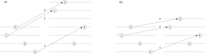
Figure 1: Change the state from $[2,1,3,4]$ to $[2,1,4,3]$ by increasing cell levels. (a) Using the “push-to-top” operations. The labels beside the three edges show the order of the three “push-to-top” operations. (b) Using the more moderate “minimal-push-up” operations.

With the recent application to flash memories, the rank-modulation scheme has gained renewed interest as evident in the recent series of papers [2, 3, 7, 6, 5, 1]. Basically, instead of a conventional multi-level cell in which a symbol in the input alphabet is represented by the charge level of one cell, in rank modulation, the stored information is represented by the permutation induced by the relative charge levels of several cells. The scheme, first described in [2] in the context of flash memory, works in conjunction with a simple cell-programming operation called “push-to-the-top”, which raises the charge level of a single cell above the rest of the cells. It was suggested in [2] that this scheme speeds up cell programming by eliminating the over-programming problem. In addition, it also reduces corruption due to retention.

The cost of changing the state in the scheme – namely, the cost of the rewriting step – is measured by the number of “push-to-top” operations that are used, because it represents by how much the maximum cell level among the $n$ cells has increased [2]. It is important to minimize this cell-level increment because the cells have a physical limit that upper bounds the cell levels. The less the cell levels are increased, the more rewrites can be performed before a block erasure operation becomes necessary, and the longer the lifetime of the memory will be.

We show an example in Fig. 1 (a), where the state of $n=4$ cells needs to change from $\mathbf{u}=[2,1,3,4]$ to $\mathbf{v}=[2,1,4,3]$. (Here the cells are indexed by $1,2,\cdots,n$. And their state is denoted by the permutation $[u_{1},u_{2},\cdots,u_{n}]{\,\mathchar 12850\relax\,}S_{n}$, where cell $u_{1}$ has the highest charge level and $u_{n}$ has the lowest charge level. For $i=1,\cdots,n$, cell $u_{i}$ has rank $i$.) Three “push-to-top” operations are needed, where cell 4, cell 1 and cell 2 are pushed sequentially. They are represented by the three edges in the figure. The cost of this rewriting is 3.

We can see from the above example, however, that the “push-to-top” operation is a conservative approach. To change the state from $\mathbf{u}=[2,1,3,4]$ to $\mathbf{v}=[2,1,4,3]$, when we push cell 4, the level of cell 4 in fact only needs to be greater than cell 3. There is no need to make it greater than the levels of all the other $n-1=3$ cells (i.e., cells 1, 2 and 3). Similarly, when cell 1 is pushed, its level only needs to be greater than cell 3 and cell 4, instead of cells 2, 3 and 4. So a more moderate programming approach as shown in Fig. 1 (b) can be taken, and the increment of the cell levels (in particular, the increment of the maximum cell level) can be substantially reduced. So the cost of rewriting can be reduced, which is important for the overall rewriting performance and the longevity of the memories.

In this work, we consider a programming approach that minimizes the increase of cell levels. To change the cell state from $\mathbf{u}=[u_{1},u_{2},\cdots,u_{n}]{\,\mathchar 12850\relax\,}S_{n}$ to $\mathbf{v}=[v_{1},v_{2},\cdots,v_{n}]{\,\mathchar 12850\relax\,}S_{n}$, we program cells based on their order in $\mathbf{v}$, so that every cell’s level increases as little as possible:

• For $i=n-1,n-2,\cdots,1$ do:

  $\{$ Increase the level of cell $v_{i}$, to make it greater than the level of the cell $v_{i+1}$ $\}$.

Note that in the above programming process, when cell $v_{i}$ is programmed, cell $v_{i+1}$ already has the highest level among the cells $v_{i+1},v_{i+2},\cdots,v_{n}$. We call the programming operation here the “minimal-push-up” operation. (In comparison, if we program cell $v_{i}$ to make its level greater than the maximum level among the cells $v_{1},\cdots,v_{i-1},v_{i+1},\cdots,v_{n}$, then it becomes the original “push-to-top” operation.) The “minimal-push-up” approach is robust, too, as it has no risk of overshooting. And it minimizes increment of the maximum level of the $n$ cells (i.e., the rewrite cost).

In section II of the paper we study a discrete model of the rewrite process that allows us to define the rewrite cost of the “minimal-push-up” operation. We show that the cost equals the maximal rank increase among the elements of the initial permutation. In section III we turn to the problem of designing rewrite codes under a worst-case cost constraint. We limit ourselves to codes that assign a symbol to each one of the states, and show that such codes for a worst-case cost of 1 cannot achieve a storage capacity greater than $1-\frac{1}{n}\log_{2}(\frac{8}{3})$ bits per cell. We consider code constructions that achieve that bound for $n\leqslant 5$, where the capacity is $54\%$ higher than that of previous rank modulation codes. Finally, we show a way to generalize the construction for higher cost constraints.

II Rewrite model and the transition graph

To design coding schemes, we need a good robust discrete model for the rewriting. We present here a discrete model for measuring the rewriting cost, which is suitable for both the “push-to-top” approach and the “minimal-push-up” approach. To rigorously define the cost of a rewriting step (i.e., a state transition), we will use the concept of virtual levels. Let $\mathbf{u}=[u_{1},u_{2},\cdots,u_{n}]{\,\mathchar 12850\relax\,}S_{n}$ denote the current cell state, and let $\mathbf{v}=[v_{1},v_{2},\cdots,v_{n}]{\,\mathchar 12850\relax\,}S_{n}$ denote the new state that the cells need to change into via increasing cell levels. Let $d(\mathbf{u}\to\mathbf{v})$ denote the number of push-up operations that are applied to the cells in order to change the state from $\mathbf{u}$ into $\mathbf{v}$. For $i=1,2,\cdots,d(\mathbf{u}\to\mathbf{v})$, let $p_{i}{\,\mathchar 12850\relax\,}[n]\triangleq\{1,2,\cdots,n\}$ denote the integer and let $B_{i}\subseteq[n]\setminus\{p_{i}\}$ denote the subset, such that the $i$-th push-up operation is to increase the $p_{i}$-th cell’s level to make it greater than the levels of all the cells in $B_{i}$. (For example, for the rewriting in Fig. 1 (a), we have $d(\mathbf{u}\to\mathbf{v})=3$, $p_{1}=4$, $B_{1}=\{1,2,3\}$, $p_{2}=1$, $B_{2}=\{2,3,4\}$, $p_{3}=2$, $B_{3}=\{1,3,4\}$. And for the rewriting in Fig. 1 (b), we have $d(\mathbf{u}\to\mathbf{v})=3$, $p_{1}=4$, $B_{1}=\{3\}$, $p_{2}=1$, $B_{2}=\{3,4\}$, $p_{3}=2$, $B_{3}=\{1,3,4\}$.) Clearly, such push-up operations have no risk of overshooting.

For the current state $\mathbf{u}$, we assign the virtual levels $n,n-1,\cdots,2,1$ to the cells $u_{1},u_{2},\dots,u_{n-1},u_{n}$, respectively. The greater a cell’s level is, the greater its virtual level is. It should be noted that when the virtual level increases by one, the increase in the actual cell level is not a constant because it depends on the actual programming process, which is noisy. However, it is reasonable to expect that when we program a cell $a$ to make its level higher than a cell $b$, the difference between the two cell levels will concentrate around an expected value. (For example, a one-shot programming using hot-electron injection can achieve quite stable programming performance at high writing speed.) Based on this, we formulate a simple yet robust discrete model for rewriting, which will be an important tool for designing coding schemes.

Consider the $i$th push-up operation (for $i=1,\dots,d(\mathbf{u}\to\mathbf{v})$), where we increase the level of cell $p_{i}$ to make it greater than the levels of the cells in $B_{i}$. For any $j{\,\mathchar 12850\relax\,}[n]$, let $\ell_{j}$ denote cell $j$’s virtual level before this push-up operation. Then after the push-up operation, we let the virtual level of cell $p_{i}$ be

$$1+\max_{j{\,\mathchar 12850\relax\,}B_{i}}\ell_{j};$$

namely, it is greater than the maximum virtual level of the cells in $B_{i}$ by one. This increase represents the increment of the level of cell $p_{i}$. After the $d(\mathbf{u}\to\mathbf{v})$ push-up operations that change the state from $\mathbf{u}$ to $\mathbf{v}$, for $i=1,\dots,n$, let $\ell_{i}^{\prime}$ denote the virtual level of cell $i$. We define the cost of the rewriting process as the increase in the maximum virtual level of the $n$ cells, which is

$$\max_{i{\,\mathchar 12850\relax\,}[n]}\ell_{i}^{\prime}-n=\ell_{v_{1}}^{\prime}-n.$$

Example 1

. For the rewriting process shown in Fig. 1 (a), the virtual levels of cells 1, 2, 3, 4 change as $(3,4,2,1)\to(3,4,2,5)\to(6,4,2,5)\to(6,7,2,5)$. Its cost is 3.

For the rewriting process shown in Fig. 1 (b), the virtual levels of cells 1, 2, 3, 4 change as $(3,4,2,1)\to(3,4,2,3)\to(4,4,2,3)\to(4,5,2,3)$. Its cost is 1. ∎

Figure 2: Change the state from $[1,2,3,4]$ to $[2,1,4,3]$. The labels beside the edges represent the order of the minimal-push-up operations. (a) The typical programming process, where two cells are pushed up. (b) In the rare case, if the level of cell 4 exceeds the level of cell 1, then three minimal-push-up operations are needed.

We would like to comment further on the robustness of the above discrete model. The model captures the typical behavior of cell programming. Yet when the minimal-push-up operations are used, the number of cells to push in practice is not always a constant when the old and new states $\mathbf{u},\mathbf{v}$ are given. An example is shown in Fig. 2, where the state needs to change from $\mathbf{u}=[1,2,3,4]$ to $\mathbf{v}=[2,1,4,3]$. The typical programming process is shown in Fig. 2 (a), where two cells – cell 4 and then cell 2 – are pushed up sequentially. (Note that based on the discrete model, the rewriting cost is 1. This is consistent with the increase of the maximum cell level here.) But as shown in Fig. 2 (b), in the rare case where cell 4’s level is significantly over-raised to the extent that it exceeds the level of cell 1, cell 1 will also be programmed, leading to three minimal-push-up operations in total. However, we would like to show that above discrete model is still a robust model for the following reasons. First, in this paper we focus on the typical (i.e., most probable) behavior of cell programming, where the rewriting cost matches the actual increase of the maximum cell level well. In the rare case where cell levels are increased by too much, additional load balancing techniques over multiple cell groups can be used to handle it. Second, the rare case – that a cell’s level is overly increased – can happen not only with the minimal-push-up operation but also with the push-to-top operation; and its effect on the increment of the maximal cell level is similar for the two approaches. So the discrete model still provides a fair and robust way to evaluate the rewriting cost of different state transitions.

In the rest of the paper, we present codes based on state transitions using the minimal-push-up operations. Given two states $\mathbf{u}=[u(1),u(2),\cdots,u(n)]{\,\mathchar 12850\relax\,}S_{n}$ and $\mathbf{v}=[v(1),v(2),\cdots,v(n)]{\,\mathchar 12850\relax\,}S_{n}$, let $C(\mathbf{u}\to\mathbf{v})$ denote the cost of changing the state from $\mathbf{u}$ to $\mathbf{v}$. (Note that $u(\cdot),v(\cdot)$ are both functions. Let $u^{-1},v^{-1}$ be their inverse functions.) The value of $C(\mathbf{u}\to\mathbf{v})$ can be computed as follows. Corresponding to the old state $\mathbf{u}$, assign virtual levels $n,n-1,\cdots,1$ to the cells $u(1),u(2),\cdots,u(n)$, respectively. For $i=1,2,\cdots,n$, let $\ell_{i}$ denote the virtual level of cell $i$ corresponding to the new state $\mathbf{v}$. Then based on the programming process described previously, we can compute $\ell_{1},\cdots,\ell_{n}$ as follows:

1. For $i=1,2,\cdots,n$ do:

   $\{$ $\ell_{u(i)}\leftarrow n+1-i$. $\}$

2. For $i=n-1,n-2,\cdots,1$ do:

   $\{$ $\ell_{v(i)}\leftarrow\max\{\ell_{v(i+1)}+1,~{}\ell_{v(i)}\}$. $\}$

Then we have

$$C(\mathbf{u}\to\mathbf{v})=\ell_{v(1)}-n.$$

It is simple to see that $0\leqslant C(\mathbf{u}\to\mathbf{v})\leqslant n-1$. An example of the rewriting cost is shown in Fig. 3.

Figure 3: State diagram for the states of three cells, where every edge represents a state transition of cost 1. The dashed edges are transitions obtained by “minimal-push-up” operations but not “push-to-top” operations.

In the following theorem we present an equivalent definition of the cost. According to the theorem, the cost is equal to the maximal increase in rank among the cells.

Theorem 1

.

$$C(\mathbf{u}\to\mathbf{v})=\max_{i{\,\mathchar 12850\relax\,}[n]}(v^{-1}(i)-u^{-1}(i)).$$

Proof:

Assume by induction on k that

$$\ell_{v(k)}=n+1-k+\max_{i{\,\mathchar 12850\relax\,}[k,\dots,n]}(i-u^{-1}(v(i))).$$

In the base case, $k=n$, and $\ell_{v(n)}=n+1-n+\max_{i{\,\mathchar 12850\relax\,}[n,\dots,n]}(i-u^{-1}(v(i)))=1+n-u^{-1}(v(n)).$ We can see that this is in fact the result of the programming process. Now we assume that the expression is true for $k$. For $k-1$, by the programming process,

$$\ell_{v(k-1)} =\max\{\ell_{v(k)}+1,n+1-u^{-1}(v(k-1))\}$$

$$=\max\{n+1-k+\max_{i{\,\mathchar 12850\relax\,}[k,\dots,n]}(i-u^{-1}(v(i)))+1,$$

$$\qquad\qquad n+1-u^{-1}(v(k-1))\}$$

by the induction assumption

$$=n+1-(k-1)+$$

$$\max\{\max_{i{\,\mathchar 12850\relax\,}[k,\dots,n]}(i-u^{-1}(v(i))),k-1-u^{-1}(v(k-1))\}$$

$$=n+1-(k-1)+\max_{i{\,\mathchar 12850\relax\,}[k-1,\dots,n]}(i-u^{-1}(v(i)))$$

and the induction is proven.

Now we assign $\ell_{v(1)}$ in the definition of the cost:

$$C(\mathbf{u}\to\mathbf{v}) =\ell_{v(1)}-n$$

$$=n+1-1+\max_{i{\,\mathchar 12850\relax\,}[1,\dots,n]}(i-u^{-1}(v(i)))-n$$

$$=\max_{i{\,\mathchar 12850\relax\,}[n]}(v^{-1}(i)-u^{-1}(i))$$

 

Codes for rewriting data based on the “push-to-top” operation were studied in [2]. Since the “minimal-push-up” approach has lower rewriting cost than the “push-to-top” operation, we can construct rewrite codes with higher rates.

In order to discuss rewriting, we first need to define a decoding scheme. It is often the case that the alphabet size used by the user to input data and read stored information differs from the alphabet size used as internal representation. In our case, data is stored internally in one of $n!$ different permutations. Let us assume the user alphabet is $Q=\{1,2,\dots,q\}$. A decoding scheme is a function $D:S_{n}\rightarrow Q$ mapping internal states to symbols from the user alphabet. Suppose the current internal state is $\mathbf{u}{\,\mathchar 12850\relax\,}S_{n}$ and the user inputs a new symbol $\alpha{\,\mathchar 12850\relax\,}Q$. A rewriting operation given $\alpha$ is now defined as moving from state $\mathbf{u}{\,\mathchar 12850\relax\,}S_{n}$ to state $\mathbf{v}{\,\mathchar 12850\relax\,}S_{n}$ such that $D(\mathbf{v})=\alpha$. The cost of the rewriting operation is $C(\mathbf{u}\rightarrow\mathbf{v})$.

Next, we define a few terms. Define the transition graph $G_{n}=(V_{n},A_{n})$ as a directed graph with $V_{n}=S_{n}$, i.e., with $n!$ vertices representing the permutations in $S_{n}$. There is a directed edge $\mathbf{u}\rightarrow\mathbf{v}$ if and only if $C(\mathbf{u}\rightarrow\mathbf{v})=1$. Note that $G_{n}$ is a regular digraph. Given a vertex $\mathbf{u}{\,\mathchar 12850\relax\,}V_{n}$ and an integer $r{\,\mathchar 12850\relax\,}\{0,1,\cdots,n-1\}$, we define the ball $B_{n,r}(\mathbf{u})$ as $B_{n,r}(\mathbf{u})=\{\mathbf{v}{\,\mathchar 12850\relax\,}V_{n}|C(\mathbf{u}\rightarrow\mathbf{v})\leqslant r\}$.

Theorem 2

.

$$|B_{n,r}(\mathbf{u})|=r!(r+1)^{n-r}$$

Proof:

We use induction on $n$. When $n=2$ the statement is trivial. (So is it when $n=r+1$, where $|B_{r+1,r}(\mathbf{u})|=(r+1)!$.) Now we assume that the statement is true for $n\leqslant n_{0}$, and consider $n=n_{0}+1$ and $n>r+1$. Let $\mathbf{u}=[u(1),u(2),\cdots,u(n)]{\,\mathchar 12850\relax\,}S_{n}$, and without loss of generality (w.l.o.g.) let $u(1)=n$. Let $\mathbf{v}=[v(1),v(2),\cdots,v(n)]{\,\mathchar 12850\relax\,}B_{n,r}(\mathbf{u})$. Let $\hat{\mathbf{u}}=[u(2),u(3),\cdots,u(n)]{\,\mathchar 12850\relax\,}S_{n-1}$, and let $\hat{\mathbf{v}}{\,\mathchar 12850\relax\,}S_{n-1}$ be obtained from $\mathbf{v}$ by removing the element $u(1)=n$. By Theorem 1, the first element in $\mathbf{u}$, namely $u(1)=n$, can take one of the first $r+1$ positions in $\mathbf{v}$. Given that position, there is a one-to-one mapping between pushing-up the remaining $n-1$ elements from $\mathbf{u}$ to $\mathbf{v}{\,\mathchar 12850\relax\,}S_{n}$ and pushing-up those $n-1$ elements from $\hat{\mathbf{u}}$ to $\hat{\mathbf{v}}{\,\mathchar 12850\relax\,}S_{n-1}$, and we have $C(\hat{\mathbf{u}}\to\hat{\mathbf{v}})=C(\mathbf{u}\to\mathbf{v})\leqslant r$. So we get $|B_{n,r}(\mathbf{u})|=(r+1)|B_{n-1,r}(\hat{\mathbf{u}})|=\cdots=(r+1)^{n-r-1}\cdot(r+1)!=r!(r+1)^{n-r}$.   

Note that given $\mathbf{u}$, $|\{\mathbf{v}{\,\mathchar 12850\relax\,}S_{n}||\mathbf{v}^{-1}(i)-\mathbf{u}^{-1}(i)|\leqslant r\;\mbox{for}\;1\leqslant i\leqslant n\}|$ is the size of the ball under infinity norm. When $r=1$, that size is known to be a Fibonacci number [4].

In addition, we note that $|B_{n,1}(\mathbf{u})|=2^{n-1}$. Therefore, the out-degree of each vertex in $G_{n}$ is $2^{n-1}-1$. In comparison, when we allow only the “push-to-the-top” operation, $|B_{n,1}(\mathbf{u})|=n$. Hence we get an exponential increase in the degree, which might lead to an exponential increase in the rate of rewrite codes. In the next section we study rewrite codes under a worst-case cost constraint.

III Worst-case decoding scheme for rewrite

In this section, we study codes where the cost of the rewrite operation is limited by $r$.

III-A The case of $n\leqslant 4$

We start with the case of $r=1$. The first non-trivial case for $r=1$ is $n=3$. However, for this case the additional “minimal-push-up” transitions do not allow for a better rewrite code. An optimal construction for a graph with only the “push-to-top” transitions was described in [2]. That construction assigns a symbol to each state according to the first element in the permutation, for a total of 3 symbols. It is easy to see that this construction is also optimal for a graph with the “minimal-push-up” transitions.

For greater values of $n$, in order to simplify the construction, we limit ourselves to codes that assign a symbol to each of the $n!$ states. We call such codes full assignment codes. Note that better codes for which not all the states are assigned to symbols might exist. When all of the states are assigned to symbols, each state must have an edge in $A_{n}$ to at least one state labelled by each other symbol. We define a set of vertices $D$ in $G_{n}$ as a dominating set if any vertex not in $D$ is the initial vertex of an edge that ends in a vertex in $D$. Every denominating set is assigned to one symbol. Our goal is to partition the set of $n!$ vertices into the maximum number of dominating sets. We start by presenting a construction for $n=4$.

Construction 1

.  Divide the 24 states of $S_{4}$ into 6 sets of 4 states each, where each set is a coset of $\langle(1,2,3,4)\rangle$, the cyclic group generated by $(1,2,3,4)$. Map each set to a different symbol.

Theorem 3

. Each set in Construction 1 is a dominating set.

Proof:

Let $I_{d}$ be the identity permutation, $g=(1,2,3,4)$ and $G=\langle g\rangle$. For each $\mathbf{h}{\,\mathchar 12850\relax\,}S_{4}$, $\mathbf{h}G$ is a coset of $G$. For each $\mathbf{v}=[v(1),\cdots,v(n)]{\,\mathchar 12850\relax\,}\mathbf{h}G$ and each $\mathbf{u}=[u(1),\cdots,u(n)]{\,\mathchar 12850\relax\,}S_{4}$ such that $u(1)=v(1)$, $\mathbf{u}$ has an edge to either $\mathbf{v}$ or $\mathbf{v}*g$. For example, in the coset $I_{d}G=G$, for $\mathbf{v}=I_{d}$ and $\mathbf{u}{\,\mathchar 12850\relax\,}S_{n}$ such that $u(1)=v(1)=1$, if $u(2)$ is 2 or 3, $\mathbf{u}$ has an edge to $I_{d}=[1,2,3,4]$, and if $u(2)=4$, $\mathbf{u}$ has an edge to $I_{d}*g=[4,1,2,3]$. Since $G$ is a cyclic group of order 4, for every $\mathbf{u}{\,\mathchar 12850\relax\,}S_{4}$ there exists $\mathbf{v}{\,\mathchar 12850\relax\,}\mathbf{h}G$ such that $u(1)=v(1)$, and therefore $\mathbf{h}G$ is a dominating set.   

For $k{\,\mathchar 12850\relax\,}[n]$ and $B\subseteq S_{n}$, we define

$$Pref_{k}(B)=\{t|\mathbf{s}=tu\;\mbox{for}\;|u|=k\;\mbox{and}\;\mathbf{s}{\,\mathchar 12850\relax\,}B\}$$

where $t,u$ are segments of the permutation $\mathbf{s}$. For example, $Pref_{3}(\{[1,2,3,4,5],[1,2,3,5,4],[1,3,2,4,5]\})=\{[1,2],[1,3]\}$.

We provide a lower bound to a dominating set’s size.

Theorem 4

. If $D$ is a dominating set of $G_{n}$, then

$$|D|\geqslant\frac{n!}{\frac{3}{4}\cdot 2^{n-1}}.$$

Proof:

Each $p_{3}{\,\mathchar 12850\relax\,}Pref_{3}(S_{n})$ is a prefix of 3 different prefixes in $Pref_{2}(S_{n})$. For example, for $n=5$, $[1,2]$ is a prefix of $\{[1,2,3],[1,2,4],[1,2,5]\}$. Each $\mathbf{v}{\,\mathchar 12850\relax\,}D$ dominates $2^{n-2}$ prefixes in $Pref_{2}(S_{n})$. For example, for $n=4$, every permutation that start with $[1,2],[1,3],[2,1]$ or $[2,3]$ has an edge to $[1,2,3,4]$. This set of prefixes can be partitioned into sets of two members, each sharing the same prefix in $Pref_{3}(S_{n})$. We look at one such set $B_{2}=\{p_{2,1},p_{2,2}\}$, and denote by $p_{3}$ the only member of $Pref_{3}(B_{2})$. Since $D$ is a dominating set, all of the members of $Pref_{2}(S_{n})$ are dominated. Therefore, the third prefix $p_{2,3}\notin B_{2}$ such that $\{p_{3}\}=Pref_{3}(\{B_{2},p_{2,3}\})$ is dominated by some $\mathbf{u}{\,\mathchar 12850\relax\,}D$, $\mathbf{u}\neq\mathbf{v}$. Moreover, $\mathbf{u}$ dominates also one of the prefixes in $B_{2}$. Therefore, at least half of the prefixes in $Pref_{2}(S_{n})$ that $\mathbf{v}$ dominates are also dominated by at least one other member of $D$. We denote by $X_{\mathbf{v}}$ the set of prefixes in $Pref_{2}(S_{n})$ that are dominated by $\mathbf{v}$ and not by any $\mathbf{u}\neq\mathbf{v}$ such that $\mathbf{u}{\,\mathchar 12850\relax\,}D$, and denote by $Y_{\mathbf{v}}$ the prefixes in $Pref_{2}(S_{n})$ that are also dominated by at least one such $\mathbf{u}\neq\mathbf{v}$. We further define $X=\sum_{\mathbf{v}{\,\mathchar 12850\relax\,}D}{|X_{\mathbf{v}}|}$ and $Y=\sum_{\mathbf{v}{\,\mathchar 12850\relax\,}D}{|Y_{\mathbf{v}}|}$. We have shown that $|X_{\mathbf{v}}|\leqslant 2^{n-3}$; so $X\leqslant 2^{n-3}|D|$. In addition, we also know that $|X_{\mathbf{v}}|+|Y_{\mathbf{v}}|=2^{n-2}$, so $X+Y=2^{n-2}|D|$. By the definition of $Y_{\mathbf{v}}$, we know that $\left|\bigcup_{\mathbf{v}{\,\mathchar 12850\relax\,}D}{Y_{\mathbf{v}}}\right|\leqslant\frac{Y}{2}$, because every element in the above union of sets appears in at least two of the sets. So we get $\frac{n!}{2}=|Pref_{2}(S_{n})|=\left|\bigcup_{\mathbf{v}{\,\mathchar 12850\relax\,}D}{X_{\mathbf{v}}}\right|+\left|\bigcup_{\mathbf{v}{\,\mathchar 12850\relax\,}D}{Y_{\mathbf{v}}}\right|\leqslant X+\frac{Y}{2}=X+2^{n-3}|D|-\frac{X}{2}=\frac{X}{2}+2^{n-3}|D|\leqslant\left(2^{n-4}+2^{n-3}\right)|D|=3\cdot 2^{n-4}|D|$. Therefore $|D|\geqslant\frac{n!}{3\cdot 2^{n-3}}$.   

Using the above bound, we can show by a simple calculation that the rate of any full assignment code $\mathcal{C}$ is $R(\mathcal{C})\leqslant 1-\frac{1}{n}\log_{2}{\frac{8}{3}}$ bits per cell. For the case of $n=4$, we see that $|D|\geqslant 4$. Therefore Construction 1 is an optimal full assignment code.

III-B The case of $n=5$

In the case of $n=5$, a dominating set consists of at least $\frac{5!}{3\cdot 2^{5-3}}=10$ members. We present an optimal full assignment code construction with dominating sets of 10 members.

Construction 2

. Divide the 120 states of $S_{5}$ into 12 sets of 10 states each, where each set is composed of five right cosets of $\langle(4,5)\rangle$, and two permutations with the same parity are in the same set if and only if they belong to the same left coset of $\langle(1,2,4,3,5)\rangle$. Map each set to a different symbol.

Let $g_{1}=(4,5)$ and $g_{2}=(1,2,4,3,5)$. An example of a dominating set where each row is a right coset of $\langle g_{1}\rangle$ and each column is a left coset of $\langle g_{2}\rangle$ is:

$$\{ [1,2,3,4,5],[1,2,3,5,4]$$

$$[2,4,5,3,1],[2,4,5,1,3]$$

$$[4,3,1,5,2],[4,3,1,2,5]$$

$$[3,5,2,1,4],[3,5,2,4,1]$$

$$[5,1,4,2,3],[5,1,4,3,2]\}$$

Theorem 5

. Each set $D$ in Construction 2 is a dominating set.

Proof:

Each right coset of $\langle g_{1}\rangle$ dominates 4 prefixes in $Pref_{3}(S_{5})$. For example, the coset $\langle g_{1}\rangle=\{I_{d}=[1,2,3,4,5],g_{1}=[1,2,3,5,4]\}$ dominates the prefixes $\{[1,2],[1,3],[2,1],[2,3]\}$. We treat each coset representative as a representative of the domination over the 4 prefixes in $Pref_{3}(S_{5})$ that are dominated by the coset. According to the construction, a set of representatives in $D$ that share the same parity is a left coset of $\langle g_{2}\rangle$. Let one of the cosets of $\langle g_{2}\rangle$ in $D$ be called $C$. For each $v{\,\mathchar 12850\relax\,}C$, the subset $\{v,v*g_{2}\}$ represents a domination over the prefix $v(2)$. For example, for $v=I_{d}$, the subset $\{I_{d}=[1,2,3,4,5],I_{d}*g_{2}=[2,4,5,3,1]\}$ represent a domination over the prefix $[2]$. Since $|\langle g_{2}\rangle|=5$, $C$ represents a complete domination over $Pref_{4}(S_{5})$, and therefore $D$ is a dominating set.   

The rate of the code is

$$R=\frac{1}{5}\log_{2}{12}=0.717\quad\mbox{bits per cell}$$

III-C The case of $r\geqslant 2$

When the cost constraint is greater than 1, we can generalize the constructions studied above. We present a construction for the case $r=n-4$. The construction begins by dividing the $n!$ states $S_{n}$ into $\frac{n!}{120}$ sets, where two states are in the same set if and only if their first $n-5$ elements are the same. The sets are all dominating sets, because we can get to any set by at most $n-5$ “push-to-top” operations. We further divide each of these sets to 12 sets of 10 members, in the same way as in Construction 2, according to the the last 5 elements of the permutations. By the properties of construction 2, each of the smaller sets is still a dominating set. The rate of the code is $R=\frac{1}{n}\log_{2}{\frac{n!}{10}}$ bits per cell.

IV Conclusion

We have presented a programming method that minimizes rewriting cost for rank modulation, and studied rewrite codes for a worst-case constraint on the cost. The presented codes are optimal full-assignment codes. It remains our future research to extend the code constructions to general code length, non-full assignment codes and average-case cost constraint.

References

- [1] E. En Gad, M. Langberg, M. Schwartz, and J. Bruck, “On a construction for constant-weight gray codes for local rank modulation,” in Proceedings of the 2010 IEEE 26-th Convention of Electrical and Electronic Engineers in Israel (IEEEI2010), Eilat, Israel, Nov. 2010, p. 996.
- [2] A. Jiang, R. Mateescu, M. Schwartz, and J. Bruck, “Rank modulation for flash memories,” IEEE Trans. on Inform. Theory, vol. 55, no. 6, pp. 2659–2673, Jun. 2009.
- [3] A. Jiang, M. Schwartz, and J. Bruck, “Correcting charge-constrained errors in the rank-modulation scheme,” IEEE Trans. on Inform. Theory, vol. 56, no. 5, pp. 2112–2120, May 2010.
- [4] T. Kløve, “Spheres of permutations under the infinity norm – permutations with limited displacement,” University of Bergen, Bergen, Norway, Tech. Rep. 376, Nov. 2008.
- [5] M. Schwartz, “Constant-weight Gray codes for local rank modulation,” in Proc. 2010 IEEE Int. Symp. Information Theory, Jun. 2010, pp. 869–873.
- [6] I. Tamo and M. Schwartz, “Correcting limited-magnitude errors in the rank-modulation scheme,” IEEE Trans. on Inform. Theory, vol. 56, no. 6, pp. 2551–2560, Jun. 2010.
- [7] Z. Wang, A. Jiang, and J. Bruck, “On the capacity of bounded rank modulation for flash memories,” in Proc. 2009 IEEE Int. Symp. Information Theory, Jun. 2009, pp. 1234–1238.