Dust-Corrected Star Formation Rates of Galaxies. II. Combinations of Ultraviolet and Infrared Tracers

Abstract

We present new calibrations of far-ultraviolet (FUV) attenuation as derived from the total infrared to FUV luminosity ratio (IRX) and the FUV-NUV color. We find that the IRX-corrected FUV luminosities are tightly and linearly correlated with the attenuation-corrected H$\alpha$ luminosities (as measured from the Balmer decrement), with a rms scatter of $\pm 0.09$ dex. The ratios of these attenuation-corrected FUV to H$\alpha$ luminosities are consistent with evolutionary synthesis model predictions, assuming a constant star formation rate over 100 Myr, solar metallicity and either a Salpeter or a Kroupa IMF with lower and upper mass limits of 0.1 and 100M_⊙. The IRX-corrected FUV to Balmer-corrected H$\alpha$ luminosity ratios do not show any trend with other galactic properties over the ranges covered by our sample objects. In contrast, FUV attenuation derived from the FUV-NUV color (UV spectral slope) show much larger random and systematic uncertainties. When compared to either Balmer-corrected H$\alpha$ luminosities or IRX-corrected FUV luminosities the color-corrected FUV luminosities show $\sim 2.5$ times larger rms scatter, and systematic nonlinear deviations as functions of luminosity and other parameters. Linear combinations of 25$\micron$ and 1.4GHz radio continuum luminosities with the observed FUV luminosities are also well correlated with the Balmer-corrected H$\alpha$ luminosities. These results provide useful prescriptions for deriving attenuation-corrected star formation rates of galaxies based on linear combinations of UV and IR or radio luminosities, which are presented in convenient tabular form. Comparisons of our calibrations with attenuation corrections in the literature and with dust attenuation laws are also made.

1 INTRODUCTION

The ultraviolet (UV) continuum of galaxies traces young massive stars, and hence serves as one of the most commonly used star formation rate (SFR) indicators (e.g., Kennicutt 1998, hereafter K98). However, the severe dust attenuation in the UV significantly weakens its power for measuring the SFR. In nearby star-forming galaxies, the dust attenuation in the UV can vary from zero to several magnitudes (e.g., Buat et al. 2005; Burgarella et al. 2005). For near-UV (NUV) selected and far-infrared (FIR) selected samples, Buat et al. (2005) found that the median dust attenuations in the far-UV (FUV) are 1.1 mag and 2.9 mag respectively (see also Burgarella et al. 2005), corresponding to 64% and 93% obscuration of the FUV light respectively. Corrections for dust attenuation therefore are essential before the UV emission is used to probe the SFR.

Commonly two approaches are used to estimate the dust attenuation in the UV. The power-law slope of the UV continuum $\beta$ ($f_{\lambda}\propto\lambda^{\beta}$, at wavelengths 1300-2600$\AA$; Calzetti et al. (1994)) was the first proposed UV dust attenuation indicator (e.g., Kinney et al. 1993; Calzetti et al. 1994; Meurer et al. 1999), and is based on the assumption that the intrinsic slope $\beta$ is only sensitive to the recent star formation history and any deviation from the intrinsic value is caused by dust attenuation (e.g., Calzetti et al. 1994; Meurer et al. 1995). However, once similar analysis is extended from starburst galaxies to normal star-forming galaxies, $\beta$ will depend on the mean age of the dust-heating population, the dust/star geometry, and the dust properties (e.g., Witt, Thronson & Capuano 1992; Witt & Gordon 2000; Granato et al. 2000; Burgarella et al. 2005).

The other UV dust attenuation estimator is the ratio of IR to UV emission. This method is built on an energetic budget consideration (e.g., Meurer et al. 1999; Buat et al. 1999). According to the energy balance argument, all the starlight absorbed at UV and optical wavebands by the interstellar dust is re-emitted in the IR, so the combination of the IR luminosity and the observed UV luminosity should be able to probe the dust-free UV luminosity (e.g., Wang & Heckman 1996; Heckman et al. 1998), which then can be used in turn to estimate the dust attenuation by comparing to the observed UV luminosity. Compared to $\beta$, the IR/UV ratio is a more reliable dust attenuation indicator because it is almost independent of the dust properties and the relative distribution of dust and stars (e.g., Buat & Xu 1996; Gordon et al. 2000; Witt & Gordon 2000; Cortese et al. 2008). However, the IR/UV ratio does depend on the age of the dust heating populations (e.g., Cortese et al. 2008; B. D. Johnson et al. 2011, in preparation). The non-ionizing UV emission is mainly from stars younger than a few hundred million years, whereas by contrast the IR emission can be from dust heated by stars over a wide age range, including not only young stars that emit a bulk of their bolometric luminosities in the UV but also evolved stars that radiate only a small fraction of their bolometric energies in the UV or even do not contribute to the UV emission at all.

Since the introduction of these two methods many efforts have been made to calibrate the relations between UV attenuation and the IR/UV ratio or $\beta$ (or equivalently FUV-NUV color) or the IR/UV versus $\beta$ relation (e.g. Meurer et al. 1999; Buat et al. 1999; Gordon et al. 2000; Bell 2002; Kong et al. 2004; Calzetti et al. 2005; Seibert et al. 2005; Cortese et al. 2006; Boissier et al. 2007; Gil de Paz et al. 2007; Johnson et al. 2007a,2007b; Panuzzo et al. 2007; Salim et al. 2007,2009; Treyer et al. 2007; Boquien et al. 2009; Buat et al. 2010; Takeuchi et al. 2010). Most of the calibrations are either purely based on theoretical models or based on comparisons of multi-wavelength photometry with stellar population synthesis models. For example, Meurer et al. (1999) obtained a relationship between FIR/FUV and the attenuation at FUV ($A_{\rm FUV}$) using the stellar population synthesis models of Leitherer & Heckman (1995) and then they derived an $A_{\rm FUV}$–$\beta$ relation using this FIR/FUV–based $A_{\rm FUV}$ for starburst galaxies. Buat et al. (2005) derived $A_{\rm UV}$–IR/UV relations for star-forming galaxies at FUV and NUV wavebands based purely on stellar population synthesis modelling. Salim et al. (2007) estimated the UV attenuation by comparing the observed spectral energy distributions (SEDs) to modelled SEDs and then based on this UV attenuation they obtained $A_{\rm FUV}$–$\beta$ relations for star-forming galaxies selected spectroscopically or using NUV-r color. Other studies that use different samples or types of galaxies to derive prescriptions for estimating UV attenuation either from IR/UV or from $\beta$ (or equivalently FUV-NUV color) include Burgarella et al. 2005, Seibert et al. 2005 and Cortese et al. 2008. As discussed earlier, the IR/UV ratio and the FUV-NUV color are dependent on the age of the dust heating populations, so calibrations based on different samples, regardless of the methods adopted, should account for this age effect. The considerable inconsistencies between the above prescriptions (see Section 6.2) imply that the age difference of the stellar populations of the samples used was largely taken into account, and these prescriptions have been applied widely in the literature to correct for UV attenuations (e.g., Bell & Kennicutt 2001; Iglesias-Páramo et al. 2006). However, the reliability and accuracy of these corrections need to be evaluated using an independent set of attenuation estimates.

In the literature an independent attenuation estimate, the attenuation in the H$\alpha$ line (A_Hα) as derived from the Balmer decrement ratio, has also been used to estimate the attenuation in the UV. To achieve this, two methods have been employed. One is based on the idea that the SFR derived from attenuation-corrected H$\alpha$ luminosity matches that from attenuation-corrected UV luminosity (e.g., Buat et al. 2002; Treyer et al. 2007). Using this method, Buat et al. (2002) explored the possibility of using the observed H$\alpha$/UV ratio to estimate the UV attenuation. Treyer et al. (2007) employed this method to estimate the UV attenuation and then built an A_FUV – FUV-NUV relation. The alternative approach is to obtain a scale factor between the attenuations in the H$\alpha$ line and in the UV by assuming a dust attenuation law (e.g., Buat et al. 2002). Both methods are strongly model-dependent, however, which adds to systematic uncertainties in the results. The UV attenuation derived using the first method, i.e., by matching the UV and H$\alpha$ derived SFRs, depends not only on the Balmer-based attenuation estimates in the H$\alpha$ line but also on the conversions of H$\alpha$ and UV luminosities to SFRs. On the other hand, the second method rests heavily on the form of the assumed dust attenuation law.

In this paper we take advantage of the large sets of multi-wavelength observations of nearby galaxies, including UV, IR and optical spectra derived Balmer decrement ratios, to calibrate IR/UV and FUV-NUV as UV attenuation estimators empirically in a self-consistent way. The calibrations derived this way are purely empirical, and depend only weakly on the Balmer-derived A_Hα.

This paper is the second of a series, in which we aim to use multi-wavelength measurements of nearby galaxies to derive attenuation corrections. In Kennicutt et al. (2009; hereafter Paper I), we used the Spitzer Infrared Nearby Galaxies Survey (SINGS; Kennicutt et al. 2003) and an integrated spectral survey sample from Moustakas & Kennicutt (2006; hereafter MK06) to calibrate the combinations of the optical emission lines (H$\alpha$ and [OII]$\lambda$3727) and the IR or radio continuum emission as attenuation-corrected SFR indicators. We found that the dust attenuation corrected H$\alpha$ luminosities, as derived from the Balmer decrement ratios, can be closely traced by the combinations of the observed H$\alpha$ emission-line luminosities with 24$\micron$, total IR (TIR; the bolometric luminosity over the wavelength range 3-1100$\micron$), and even 8$\micron$ IR luminosities, with rms scatters $\sim$ 0.1 dex.

In this paper we derive new calibrations for UV attenuation corrections as derived from the IR/UV ratio and the FUV-NUV color as described above, and test the consistency of the SFRs computed from IR/UV or FUV-NUV corrected UV luminosities to those from Balmer-corrected H$\alpha$ luminosities. Compared to FUV, NUV can be contributed by more evolved stars ($\sim 1$ Gyr). Therefore we mainly focus on FUV in this paper. But we also explore the reliability of using IR/NUV as a dust attenuation estimator as NUV is sometimes used as a SFR indicator. The remainder of this paper is organized as follows. In Section 2 we describe the sample, and describe how the UV flux densities were obtained. The calibrations of the relationships between the attenuation in the FUV and the TIR to FUV ratio, the UV color are shown in Section 3. In Section 4 we apply the calibrations derived in Section 3 to two samples of nearby galaxies to test the reliability of using these attenuation-corrected FUV luminosities as SFR indicators. Second order effects of these attenuation-corrected FUV luminosities relative to the Balmer-corrected H$\alpha$ luminosities are also investigated in Section 4. At last, we explore the possibility of using the combinations of FUV with monochromatic MIR luminosities 25$\micron$ (or 24$\micron$) and radio continuum to estimate dust attenuations in Section 4. In Section 5, the reliability of using NUV luminosity as a SFR indicator is discussed. In Section 6 the limitations and the range of applicability of the use of the calibrations are discussed. Comparisons of our calibrations to those in the literature, to the attenuation curve of Calzetti et al. 2000 and to results based on SFR matching method are made in Section 6 as well. Finally we summarize our results in Section 7. For distance estimates, we assume ${\rm H}_{0}=70{\rm km\,s^{-1}\,Mpc^{-1}}$ with local flow corrections.

2 SAMPLE AND DATA

Our galaxies are drawn from the integrated spectrophotometric survey by MK06 and the SINGS survey. The survey information and the selection criteria were described in Paper I. We briefly list them here for completeness. The MK06 survey observed 417 galaxies, which were selected to cover the full range of optical spectral characteristics found in the local galaxies, using a long-slit drift-scanning technique. The reduced spectrum was integrated over a rectangular aperture that includes most or all of the emission of the galaxy. The SINGS survey was a multi-wavelength survey from the FUV to the FIR and it was composed of 75 nearby galaxies that cover wide ranges in morphological type, luminosity, star formation rate and dust opacity. In this paper series we aim to use attenuation-corrected H$\alpha$ luminosities, as derived from Balmer decrement ratios, to calibrate combinations of optical emission lines or UV continuum and the IR or radio continuum as dust attenuation corrected SFR indicators. Therefore several criteria were employed to ensure the quality of the data (1) galaxies without detectable H$\alpha$ emission were excluded, (2) in order to obtain reliable measurements of the Balmer decrement ratios, galaxies with low signal to noise ratio spectra at H$\beta$ (S/N $\lesssim$ 15) were removed, (3) galaxies classified as active galactic nuclei (AGNs) or AGN-starburst composites (c.f. Moustakas et al. 2006; Kewley et al. 2001; Kauffmann et al. 2003) were excluded, and (4) galaxies with lower than 3$\sigma$ detections at 25$\micron$ were removed. Given that we will calibrate the attenuation estimates in the UV from the TIR/UV ratio and the FUV-NUV color, FUV and NUV photometric data are needed. Some of the galaxies used in Paper I have not been observed by the Galaxy Evolution Explorer (GALEX; Martin et al. 2005) so they are not included in the following analyses.

Similar to Paper I, IR data and the attenuation corrected H$\alpha$ luminosities from H$\alpha$/H$\beta$ ratios are required. The compilation of H$\alpha$ fluxes, [NII]/H$\alpha$, H$\alpha$/H$\beta$ and IR data has been described in detail in that paper. As stated in Paper I, most of the galaxies in the MK06 sample have not been observed with Spitzer. To maximize the uniformity of the data, only the Infrared Astronomical Satellite (IRAS) data were used to derive the TIR luminosities, which was estimated using a weighted sum of IRAS 25$\micron$ , 60$\micron$ and 100$\micron$ emission following Dale & Helou (2002; equation (5) of their paper). We will discuss possible systematics introduced by using IRAS-based TIR luminosities in Section 6.6. We also provide calibrations for the combinations of the monochromatic MIR (IRAS 25$\micron$ or Spitzer 24$\micron$) luminosities and the observed UV luminosities in Section 4.3. This is useful when FIR data are not available. As shown in Paper I, the IRAS 25$\micron$ luminosity (${\rm L}(\lambda)=\nu{\rm L}_{\nu}$) and the Spitzer/Multiband Imaging Photometer for Spitzer (MIPS) 24$\micron$ luminosity can be used interchangeably. Given that Spitzer/MIPS 24$\micron$ photometry is more sensitive than IRAS we use those measurements in preference to IRAS for the SINGS galaxies in Section 4.3. Spitzer/MIPS 24$\micron$ measurements were also performed for the central 20″ $\times$ 20″ regions of the SINGS galaxies in Paper I, and they are also used in this paper (Section 4.3).

For galaxies selected from the MK06 sample, we identified their counterparts in the UV from GALEX GR4. GALEX performs imaging observations at FUV and NUV bands, centered at 1528$\AA$ and 2271$\AA$ respectively, with a circular field of view of $1\fdg 2$ diameter (Martin et al. 2005). GR4 includes images taken from the All-sky Imaging Survey (AIS), Medium Imaging Survey (MIS), Nearby Galaxies Survey (NGS), Deep Imaging Survey (DIS) and Guest Investigators Survey (GI). Since artifacts appear much more frequently at the edge of the field of view, only galaxies within a radius of $0\fdg 55$ from the field center were selected (Morrissey et al. 2007). Because of the overlap in coverage of these surveys, sometimes there were more than one image available. In such cases, we used the one with the longest exposure time in the FUV. After this process we were left with 98 galaxies (54 in AIS, 4 in MIS, 22 in NGS, 2 in DIS and 16 in GI) out of the 113 star-forming galaxies selected from the MK06 sample. But NGC 1003, which is in AIS, was excluded later because of artifact contamination in its FUV image. So the final sample consists of 97 objects, with 53 in the AIS survey.

Intensity (-int) and sky background (-skybg) images at FUV and NUV bands were retrieved from the Multimission Archive at Space Telescope Science Institute (MAST) website (Morrissey et al. 2007). Sky background was subtracted before performing photometry. In order to obtain the UV fluxes from the same region as H$\alpha$, the rectangular apertures used in the integrated spectra observations by MK06 were adopted in the UV photometry. Foreground stars within the apertures, identified by comparing the NUV and the Digitized Sky Survey (DSS) optical images, were masked during the photometry. The FUV and NUV magnitude zero points listed in Morrissey et al. (2007) were used to convert intensities into magnitudes. The high-resolution relative response images (-rrhr) from MAST were used to estimate the uncertainties in the photometry. The FUV and NUV flux densities were corrected for Galactic extinction using the Schlegel et al. (1998) dust map and the Galactic extinction curve derived by Cardelli et al. (1989) for a total-to-selective extinction of $R_{V}=3.1$ (c.f., Gil de Paz et al. 2007). Specifically, ${\rm A_{FUV}=7.9E(B-V)}$ and ${\rm A_{NUV}=8.0E(B-V)}$. The Galactic extinction corrected FUV and NUV flux densities of the MK06 sample are listed in Table 1. The absolute calibration uncertainties in FUV (0.05 mag) and NUV (0.03 mag) are added in quadrature.

Since more than half of the MK06 sample galaxies (53 out of 97) were extracted from the shallow AIS survey, with exposure times of 100s, 15 times shorter than the MIS, we tested whether some of the extended UV emission was missed in AIS images compared to observations with deeper exposures. There are 43 objects in common between the AIS and the other deeper surveys. We compared their UV magnitudes measured from the AIS images and those from observations with longer exposure time in Figure 1. It is clear that the UV measurements based on the AIS images are in excellent agreement, within $\sim$20%, with those from deeper exposures, which means that the UV fluxes measured from the AIS images are not systematically under-estimated within the adopted rectangular apertures. Consequently they can be used along with the measures from deeper exposures without introducing any systematic errors.

UV flux densities for the SINGS sample were obtained from Dale et al. (2007). Those authors calculated the FUV and NUV flux densities from the surface brightness profiles derived for the GALEX Atlas of Nearby Galaxies (Gil de Paz et al. 2007). Since Dale et al. (2007) used Li & Draine (2001) reddening curve to correct for the Galactic extinction, we redid the Galactic extinction using the same recipes as those used for the MK06 sample for consistency. Applying the requirement of having both IRAS data and UV flux measurements left us with 36 objects for the SINGS sample. To avoid small number statistics and the less reliable measurements of H$\alpha$/H$\beta$ ratios for some of the SINGS objects (see Paper I), we do not use these objects to calibrate the relations in the following analyses. However we include them in the comparison to see how they behave. We also measure the FUV and NUV flux densities for the central 20″ $\times$ 20″ regions of the SINGS galaxies. It should be noted that the large absolute calibration uncertainties (0.15 mag) in Gil de Paz et al. are included in the quoted errors in FUV and NUV for SINGS sample.

3 EMPIRICALLY CALIBRATED A_FUV – TIR/FUV, FUV-NUV COLOR RELATIONS

As addressed in Section 1, prescriptions of using TIR/FUV as a dust attenuation indicator are usually derived under various model assumptions. In this section, we employ a new method to derive such prescriptions empirically and avoid most of the systematic model dependencies. Our method is based on the statistical correlation between the FUV attenuation estimated from the TIR/FUV ratio and that as derived from the FUV-NUV color. By deriving the prescriptions based on a sample of nearby star-forming galaxies, we virtually assume an average stellar population and dust attenuation curve of a certain type of galaxies. Therefore our calibrations are probably not applicable for other types of galaxies (see Section 6).

We adopt the convention of infrared excess IRX from Meurer et al. (1995)

$${\rm IRX}=\log[{\rm L(TIR)/L(FUV)_{obs}}],$$ (1)

where the observed FUV luminosity takes the common definition of monochromatic luminosity ${\rm L(FUV)_{obs}}=\nu{\rm L}_{\nu}(1528\AA)$.

According to an energy balance argument, the dust attenuation in the FUV, ${\rm A_{FUV}}$, can be estimated from the IRX using the following form

$${\rm A_{FUV}}=2.5\log(1+a_{\rm FUV}\cdot 10^{\rm IRX}),$$ (2)

where $a_{\rm FUV}$ is a scale parameter, whose meaning is explained below. This approach is similar to that presented in Paper I for the combination of the observed H$\alpha$ luminosity and the TIR luminosity. As stated in Paper I, such an expression is a simple approximation to a much more complicated radiative transfer process. To better understand the underlying physical foundations of eq. (2), we adopt the relevant equations from Paper I and adapt them to the case of FUV.

We first define a scale parameter $\eta$, which is the fraction of the bolometric luminosity that is emitted in the FUV, i.e., the inverse of the bolometric correction

$${\rm L(FUV)_{corr}=\eta_{FUV}L_{bol}},$$ (3)

where ${\rm L(FUV)_{corr}}$ represents the intrinsic (extinction-free) FUV luminosity and ${\rm L_{bol}}$ denotes the bolometric luminosity.

Under the assumption of a foreground dust screen approximation, the observed luminosity can be expressed as

$${\rm L(FUV)_{obs}=L(FUV)_{corr}}\,{\rm e}^{-{\tau_{\rm FUV}}},$$ (4)

where $\tau_{\rm FUV}$ is an effective optical depth in the FUV, as defined by equation (4), and the corresponding attenuation in magnitudes ${\rm A_{FUV}}=1.086\,\tau_{\rm FUV}$.

The dust attenuation corrected FUV luminosity is a sum of the observed luminosity and the dust-attenuated luminosity

$${\rm L(FUV)_{corr}=L(FUV)_{obs}+L(FUV)_{corr}}\,(1-{\rm e}^{-{\tau_{\rm FUV}}}).$$ (5)

Considering the energy conservation, all the starlight reprocessed by dust is re-emitted in the IR. So the TIR luminosity can be expressed as

$${\rm L(TIR)=L_{bol}}\,(1-{\rm e}^{{-\bar{\tau}}}),$$ (6)

where $\bar{\tau}$ is the effective opacity for all of the dust-heating starlight, and is defined as

$$\bar{\tau}=-\ln\frac{\int L_{\lambda}e^{-\tau_{\lambda}}d\lambda}{\int L_{\lambda}d\lambda}.$$ (7)

This effective mean opacity depends on the star formation history of the galaxy, the dust extinction curve and the relative distribution of stars and dust.

We substitute eqs.  (3) and (6) into eq.  (5) to eliminate ${\rm L_{bol}}$ and express ${\rm L(FUV)_{corr}}$ using the observable luminosities ${\rm L(FUV)_{obs}}$ and L(TIR) and the opacities. After this exercise, the dust attenuation estimate in the FUV becomes

$${\rm A_{FUV}}=2.5\log[1+\eta_{\rm FUV}\cdot 10^{\rm IRX}{{(1-{\rm e}^{-{\tau_{\rm FUV}}})}\over{(1-{\rm e}^{-\overline{\tau}})}}].$$ (8)

By comparing eq. (2) with eq. (8), it can be seen that the coefficient $a_{\rm FUV}$ in eq. (2) is the approximation of the product of the inverse of the bolometric correction $\eta_{\rm FUV}$ and the factor ${(1-{\rm e}^{-{\tau_{\rm FUV}}})}\over{(1-{\rm e}^{-\bar{\tau}})}$.

When the FUV-NUV color is used to estimate the FUV attenuation, a linear relation between ${\rm A_{FUV}}$ and the FUV-NUV color is usually taken

$${\rm A_{FUV}}=s_{\rm FUV}\cdot{\rm(FUV-NUV)_{obs}}+i_{\rm FUV},$$ (9)

where the slope $s_{\rm FUV}$ and the intercept $i_{\rm FUV}$ are usually determined by a linear regression to the observations. The physical foundations of this relation can be understood as follows.

The color excess in FUV-NUV, E(FUV-NUV) is defined as

$${\rm E(FUV-NUV)}={\rm(FUV-NUV)_{obs}-(FUV-NUV)_{int}}={\rm A_{FUV}}-{\rm A_{NUV}},$$ (10)

where ${\rm(FUV-NUV)_{obs}}$ and ${\rm(FUV-NUV)_{int}}$ denote the observed and the attenuation-corrected FUV-NUV colors. E(FUV-NUV) relates to the color excess E(B-V) by the relation

$${\rm E(B-V)={1\over(k_{FUV}-k_{NUV})}\,E(FUV-NUV)},$$ (11)

where ${\rm k_{\lambda}=A_{\lambda}/E(B-V)}$ represents an attenuation curve. So eq. (9) has the modified form

$${\rm A_{FUV}={k_{FUV}\over(k_{FUV}-k_{NUV})}}[{\rm(FUV-NUV)_{obs}}-{\rm(FUV-NUV)_{int}}].$$ (12)

By comparing this modified equation to the original eq. (9), we can see that $s_{\rm FUV}={\rm{k_{FUV}\over(k_{FUV}-k_{NUV})}}$, which is the slope of the UV part of the attenuation curve, and $i_{\rm FUV}/s_{\rm FUV}$ is equal to the dust-free UV color, ${\rm(FUV-NUV)_{int}}$.

Since the estimated ${\rm A_{FUV}}$ from IRX and FUV-NUV should agree, the predicted relation between IRX and FUV-NUV color can be obtained by equating eq. (2) and eq. (12). Given that ${\rm k_{FUV}}$ and ${\rm k_{NUV}}$ cannot be derived separately from the fitting, $s_{\rm FUV}$ is still used in the IRX – FUV-NUV relation

$${\rm IRX}=\log[10^{0.4s_{\rm FUV}\cdot{\rm[(FUV-NUV)_{obs}-(FUV-NUV)_{int}]}}-1]-\log(a_{\rm FUV}).$$ (13)

Before we proceed to derive the parameters $a_{\rm FUV}$, ${\rm(FUV-NUV)_{int}}$ and $s_{\rm FUV}$ in eq. (13) from the observations, we discuss the implicit assumptions in our method. The comparison between eq. (2) and eq. (8) shows that the coefficient $a_{\rm FUV}$ is the approximation of the product of the inverse of the bolometric correction $\eta_{\rm FUV}$ and the factor ${(1-{\rm e}^{-{\tau_{\rm FUV}}})}\over{(1-{\rm e}^{-\bar{\tau}})}$. By deriving single values for $a_{\rm FUV}$, ${\rm(FUV-NUV)_{int}}$ and $s_{\rm FUV}$, we virtually study the average properties of this sample, without taking into account variations in star formation histories and dust attenuation curves from galaxy to galaxy, which contribute to the scatters in the observed correlations.

In order to minimize the number of free parameters in the fitting, we first estimate the intrinsic (i.e., dust-free) FUV-NUV color empirically, which is achieved by the correlation between the observed FUV-NUV color and the attenuation in the H$\alpha$ line. This method is similar to Calzetti et al. (1994) in which the unattenuated power-law slope of the UV continuum $\beta_{0}$ was estimated using the correlation between $\beta$ and the Balmer decrement ratio. This correlation between the dust reddening in the stellar continuum and in the gas content (see also Calzetti 1997 and Figure 2 below) implies that the FUV attenuation in the stellar continuum is proportional to the attenuation in the H$\alpha$ line. The proportional factor is dependent on the extinction curve and the relative distribution of stars, gas and dust, which may vary from galaxy to galaxy. Unfortunately, we cannot study this property on a galaxy-to-galaxy basis based on current data, so only an average relation is obtained (see Section 6.3).

The FUV-NUV color versus ${\rm A_{H\alpha}}$ relation is shown in Figure 2. Throughout this paper the MK06 and SINGS objects are represented by solid and open circles respectively. From this figure, we can see that the MK06 and the SINGS samples tell us different stories. The MK06 sample shows that ${\rm A_{H\alpha}}$ is correlated with FUV-NUV color, whereas the SINGS sample shows almost no correlation between these two quantities after the two reddest objects are excluded. This is not unexpected given the large calibration uncertainties of UV photometry and the way we compiled the Balmer decrement ratios for the SINGS galaxies, as described in Section 2 and Paper I. Therefore only the MK06 sample is used to derive the dust-free FUV-NUV color, as indicated in Section 2. Since the scatter is probably intrinsic, which means that the measurement errors are not the main contributors to the scatter about the regression line, an ordinary least square bisector fit method is adopted (Isobe et al. 1990; Feigelson & Babu 1992). The fitting to the MK06 sample that is plotted as a solid line in Figure 2 gives

$${\rm(FUV-NUV)}=(0.539\pm 0.029){\rm A_{H\alpha}}+(0.022\pm 0.024)$$ (14)

This indicates an intrinsic FUV-NUV color for zero attenuation of $0.022\pm 0.024$ mag. The errors quoted here in the slope and intercept were yielded by the fitting routine. The dust-free FUV-NUV color derived here is in excellent agreement with the value $0.025\pm 0.049$ mag derived by Gil de Paz et al. (2007). Those authors used the prescriptions given by Buat et al. (2005) to correct for the dust attenuation in the FUV and NUV using the TIR/FUV and TIR/NUV ratios, and found that the intrinsic FUV-NUV color for their sample is $0.025\pm 0.049$ mag on average. To understand the average stellar population of our sample galaxies, we compare the intrinsic FUV-NUV color we derived here with the stellar population synthesis predictions. By comparing to models constructed using GALAXEV by Bruzual & Charlot (2003), we find that our galaxies are $\sim$ 0.02, 0.03 and 0.04 mag redder in FUV-NUV color than a 10 Gyr old stellar population with an e-folding timescale of 5 Gyr, 10 Gyr and a constant star formation history, respectively. For a constant star formation history STARBURST99 (Leitherer et al. 1999; Vazques & Leitherer 2005) produces consistent result (see Section 6.6).

After fixing the term ${\rm(FUV-NUV)_{int}}=0.022$ in eq. (13), the coefficients $s_{\rm FUV}$ and $a_{\rm FUV}$ can be obtained by fitting eq. (13) to the data. Figure 3 shows the IRX versus FUV-NUV color relation, with the corresponding $\beta$ labelled on the top axis. The relation between FUV-NUV and $\beta$ was derived using the definition given by Kong et al. (2004) for our adopted central wavelengths for FUV and NUV (see Section 2), which has the form $\beta=2.32({\rm FUV-NUV})-2.00$. In order to have a clearer view of the average properties of the data, we overplot the IRX median, lower (25%) and upper (75%) quartiles in bins of width 0.2 mag in FUV-NUV color as open squares with error bars in Figure 3. The solid line represents the chi-square minimization fit to the MK06 sample with the deviation in the IRX minimized, which has the form defined by eq. (13) with $s_{\rm FUV}$ and $a_{\rm FUV}$ equal to $3.83\pm 0.48$ and $0.46\pm 0.12$ respectively. In order to test the effect of the adopted ${\rm(FUV-NUV)_{int}}$ on the fitting results, we varied ${\rm(FUV-NUV)_{int}}$ by $\pm 1\sigma$ about the best-fitted value, i.e., assumed ${\rm(FUV-NUV)_{int}}=0.046$ and ${\rm(FUV-NUV)_{int}}=-0.002$. It turned out that the changes in the best fitted $s_{\rm FUV}$ and $a_{\rm FUV}$ caused by these new assumptions of the ${\rm(FUV-NUV)_{int}}$ are within $\pm 1\sigma$, and the resulting IRX versus FUV-NUV color relations cannot be distinguished from that using ${\rm(FUV-NUV)_{int}}=0.022$ over the ranges of FUV-NUV color and IRX covered by our sample galaxies (see Section 6.1). Substituting the best fitted coefficients into eqs. (2) and (12), the attenuation estimates based on the IRX and the FUV-NUV color become

$${\rm A_{FUV}}=2.5\log[1+(0.46\pm 0.12)\cdot 10^{\rm IRX}],$$ (15)

and

$${\rm A_{FUV}=(3.83\pm 0.48)[{\rm FUV-NUV)_{obs}}-(0.022\pm 0.024)}].$$ (16)

4 DUST ATTENUATION CORRECTED FUV LUMINOSITY AS A SFR INDICATOR

In order to evaluate the reliability of the dust attenuation corrected FUV luminosities derived using the above calibrations as SFR indicators, we compare the IRX and FUV-NUV color corrected FUV luminosities (according to eq. (15) and (16)) with the Balmer decrement ratio corrected H$\alpha$ luminosities and investigate possible second-order trends in the residuals as functions of various properties of the galaxies in this section. Combinations of FUV with monochromatic 25$\micron$ (or 24$\micron$) infrared and radio continuum as dust attenuation measures are also explored. We note that the attenuation calibration methods we employed in Section 3 make only minimal use of the Balmer decrement data. So when we compare the dust-corrected FUV luminosities based on our calibrations with the Balmer-corrected H$\alpha$ luminosities, we are not making a circular argument.

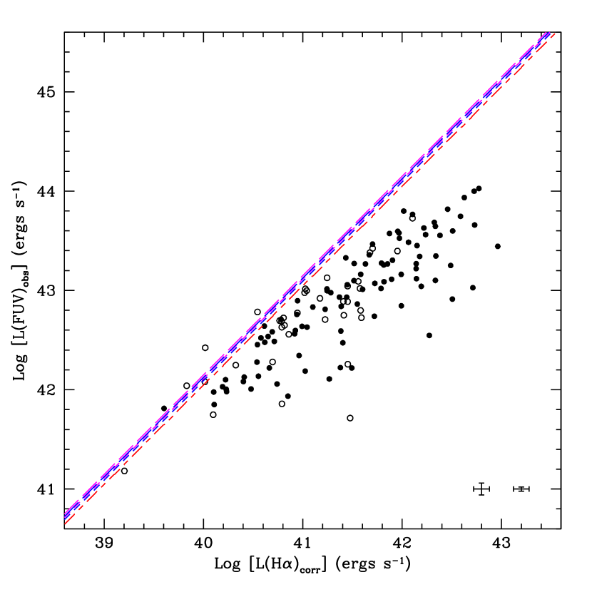
Figure 4: Observed FUV luminosities without correction for internal dust attenuation versus Balmer decrement ratio corrected H$\alpha$ luminosities for MK06 sample (solid circles) and SINGS sample (open circles). The color-coded lines represent the predicted relations (in the absence of dust attenuation in the UV) by different SFR prescriptions, same as Figure 5. The error bars in the bottom-right corner denote median errors for the MK06 sample (right) and the SINGS sample (left).

Before we proceed to compare the dust attenuation corrected FUV luminosities with the H$\alpha$ luminosities, it is interesting to see the behavior of the uncorrected FUV luminosities as a function of the Balmer decrement corrected H$\alpha$ luminosities in Figure 4, which can help us understand the importance of the attenuation corrections for this sample. The straight lines in Figure 4 are model predictions for matched SFRs as described below. Figure 4 shows that the uncorrected FUV luminosities can underestimate the SFRs by more than an order of magnitude, which varies with the intensity of the star formation activity. Galaxies with different SFRs are not equally attenuated, with more active galaxies suffering from higher attenuations. This is consistent with studies in the literature (e.g., Wang & Heckman 1996; Treyer et al. 2007). In the following part of this section, the reader will see how much will be improved with our dust attenuation corrections.

4.1 Infrared-Corrected FUV Luminosities As SFR Indicators

We compare the IRX-corrected FUV luminosities with the Balmer decrement ratio corrected H$\alpha$ luminosities in the left panel of Figure 5. It can be clearly seen that the IRX-corrected FUV luminosities correlate tightly and linearly with the Balmer-corrected H$\alpha$ luminosities with a rms scatter of $\pm 0.09$ dex.

In order to quantify the degree of consistency between the SFRs derived from the attenuation-corrected FUV and H$\alpha$ luminosities, in the left panel of Figure 5 we overplot the predicted relations from different SFR prescriptions. The red short-long dashed line represents the prediction from the widely used K98’s SFR prescriptions. The calibrations in K98 assume a Salpeter initial mass function (IMF; Salpeter 1955) with mass limits 0.1-100${\rm M}_{\odot}$, and 1990’s generation stellar evolution models (see Kennicutt et al. 1994; Madau et al. 1998). To compare with the K98’s prediction, we first construct a model under the same assumptions as K98 did, i.e., Salpeter IMF, constant star formation history lasting for 100 Myr and solar metallicity (the magenta short dashed line), using Version 5.1 of the stellar population synthesis model STARBURST99 (Leitherer et al. 1999; Vazquez & Leitherer 2005), which uses the state-of-the-art stellar evolutionary models.

Star-forming galaxies in our sample probably have experienced continuous star formation for at least 1 Gyr. In order to examine age effects, we build models with a constant star formation history lasting for 1 Gyr (represented by long dashed lines). It is worth noting that for a constant star formation history the intrinsic FUV to H$\alpha$ luminosity ratio stays constant after 1 Gyr. Therefore, the model predictions we derive by assuming a constant SFR for 1 Gyr are the same as those under the assumption of a constant SFR for longer time. Although we assume constant star formation histories here, models with exponentially declining star formation histories do not give significantly different results, as long as the SFR does not drop too rapidly. For example, for an e-folding timescale of 5 Gyr, the FUV to H$\alpha$ ratio differs from the constant star formation history by $\leq 4$% at any given age, according to our experiments based on stellar population synthesis models constructed using GALAXEV by Bruzual & Charlot (2003).

The IMF also affects the FUV/H$\alpha$ ratio. So apart from models with Salpeter IMF, models with a more realistic Kroupa IMF (Kroupa & Weidner 2003) with mass limits of 0.1-100${\rm M}_{\odot}$ are also explored (represented by lines in blue). The FUV and H$\alpha$ luminosities and their ratios are listed in Table 2.

In the left panel of Figure 5 the different models (represented by the colored lines) are difficult to separate, because of the large dynamic range in luminosities. For that reason we show in the right panel of Figure 5 histograms of the attenuation-corrected FUV to H$\alpha$ luminosity ratio, using a logarithmic scale. The MK06 and SINGS samples are represented by the solid and dotted histograms respectively. The straight lines in color are the same model predictions as those shown in the left panel of this figure. The median and mean values of the IRX-corrected FUV to H$\alpha$ luminosity ratios for the MK06 sample are 123.88 and 127.94, which are in excellent agreement with the model predictions for Kroupa IMF at 100 Myr and Salpeter IMF at 100 Myr respectively (see Table 2). However, the FUV/H$\alpha$ ratio only increases by 8% and 9% respectively for the same IMFs but older age ($\geq 1$ Gyr).

The correlation between the IRX-corrected FUV luminosities and the Balmer-corrected H$\alpha$ luminosities is so tight and linear that it is useful to test for any second order trends in the residuals as functions of various galactic properties. In Figure 6, we plot the ratios of the IRX-corrected FUV luminosities to the Balmer-corrected H$\alpha$ luminosities against the Balmer-corrected H$\alpha$ luminosities (i.e., the dust corrected SFRs; top-left panel), the Balmer-corrected H$\alpha$ luminosity densities (top-right panel), the attenuations in the H$\alpha$ line (bottom-left) and the axial ratios b/a (i.e., inclinations; bottom-right). In Figure 7, the optical spectral features – H$\alpha$ equivalent width EW(H$\alpha$) (top-left panel), 4000Å break ${\rm D_{n}}(4000{\rm\AA})$ (top-right panel), gas-phase oxygen abundance 12+log(O/H) (bottom-left panel) and the dust temperature indicator – far-infrared 60$\micron$ to 100$\micron$ flux ratio $f_{\nu}(60\micron)/f_{\nu}(100\micron)$ (bottom-right) are explored. Given that H$\alpha$ line and continuum emission are SFR and stellar mass tracers respectively, the integrated H$\alpha$ equivalent width is a measure of specific SFR (Kennicutt et al. 1994). The ${\rm D_{n}}(4000{\rm\AA})$ is often used as a reddening-insensitive rough star formation history indicator of the stellar populations (e.g., Bruzual 1983; Balogh et al. 1999; Kauffmann et al. 2003) and it correlates with the specific SFR (Brinchmann et al. 2004). In all panels the dashed line indicates the predicted FUV to H$\alpha$ luminosity ratio for a Kroupa IMF at age 100 Myr, as shown in Figure 5.

As can be seen from Figure 6 and 7, the ratios of the IRX-corrected FUV to the attenuation-corrected H$\alpha$ luminosities show no or at most marginal trends with all the parameters investigated. The rms scatters are about $\pm 0.09$ dex, which is even smaller than the average uncertainty in $\log{\rm[L(FUV)_{IRX,corr}/L(H\alpha)_{corr}]}$ ratio, $\pm 0.13$ dex, with the error introduced by using eq. (15) to correct for FUV attenuation included. This demonstrates the reliability of using the combination of the FUV and TIR luminosities as a SFR indicator. The absence of correlations implies that over the ranges of the galactic properties probed by our galaxies, either no trend exists in the dust-free FUV/H$\alpha$ ratios and the IRX method with the parameters tested above, or any trend in the dust-free FUV/H$\alpha$ ratios is compensated by that in the IRX method. Whatever it is, the SFR estimated from the IRX-corrected FUV luminosity agrees well with that derived from the Balmer-corrected H$\alpha$ luminosity, and the ratio of these dust-corrected SFRs is not a function of the galactic properties. Therefore the combined FUV and TIR luminosities can serve as a very good attenuation-corrected SFR indicator over the ranges of physical properties covered by our sample objects.

From Figure 5 to Figure 7, we note that the SINGS galaxies deviate from the MK06 galaxies systematically. The systematic deviations can be caused either by overestimates of the TIR luminosities or by underestimates of the attenuation in H$\alpha$ lines. As we showed in Paper I (Figure 2 in that paper; see also Dale et al. 2009), for cold galaxies ($f_{\nu}(60\micron)/f_{\nu}(100\micron)\leq 0.6$), the TIR luminosities measured by IRAS bands are systematically underestimated with respect to the more sensitive and accurate Spitzer/MIPS bands. Therefore using TIR luminosities based on Spitzer/MIPS measurements for the SINGS galaxies would make the SINGS galaxies deviated more. Furthermore, we did not see a correlation between the deviations and the $f_{\nu}(60\micron)/f_{\nu}(100\micron)$ colors in the bottom-right panel of Figure 7. Another piece of evidence is that the same deviations show up in the comparison of the combined FUV+25$\micron$ luminosities with the Balmer-corrected H$\alpha$ luminosities (Section 4.3), and the monochromatic 25$\micron$ luminosity measured by IRAS does not suffer from the same problem as the TIR luminosity. Therefore, the systematic deviations of the SINGS galaxies cannot result from overestimates of the TIR luminosities by IRAS. Instead, they may be due to underestimates of the attenuation in H$\alpha$ lines, caused by the noisier H$\beta$ detections.

4.2 FUV-NUV Corrected FUV Luminosities As SFR Indicators

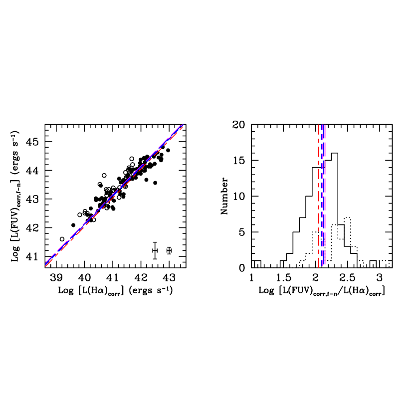
Figure 8: left panel: FUV-NUV color-corrected FUV luminosities as a function of Balmer decrement ratio corrected H$\alpha$ luminosities for MK06 sample (solid circles) and SINGS sample (open circles). The lines overplotted represent the predicted relations by different SFR prescriptions, same as those in Figure 5. The error bars in the bottom-right corner denote median errors for the MK06 sample (right) and the SINGS sample (left). right panel: Histograms of the ratios of the FUV-NUV color-corrected FUV luminosities to Balmer-corrected H$\alpha$ luminosities for MK06 sample (solid line) and SINGS sample (dotted line) in log scale. The vertical lines represent the predicted values by different SFR prescriptions, as shown in left panel. This panel is to show the differences between the models more clearly.

Similar to the analyses we did for the IRX-corrected FUV luminosities in Section 4.1, we compare the FUV-NUV color corrected FUV luminosities with the Balmer decrement ratio corrected H$\alpha$ luminosities in this subsection. Figure 8 shows the FUV-NUV corrected FUV luminosities as a function of the Balmer-corrected H$\alpha$ luminosities (left panel) and the histogram of the FUV-NUV corrected FUV to the Balmer-corrected H$\alpha$ luminosity ratio (right panel). Compared to the IRX-corrected FUV luminosities versus the Balmer-corrected H$\alpha$ luminosities relation, the correlation between the FUV-NUV corrected FUV luminosities and the Balmer-corrected H$\alpha$ luminosities is non-linear and has a much larger rms scatter of $\pm 0.23$ dex.

Figure 8 shows that the relation between the FUV-NUV color corrected FUV luminosities and the Balmer-corrected H$\alpha$ luminosities is not completely linear. The slope of the relation is less than unity, which implies that for galaxies forming stars vigorously (i.e., with high SFRs), the FUV-NUV corrected FUV luminosities will under-estimate the SFRs.

To better understand the applicability and limitation of the FUV-NUV corrected FUV luminosities as SFR measures, apart from the Balmer-corrected H$\alpha$ luminosities, we also examined the ratios of the UV color corrected FUV luminosities and the Balmer-corrected H$\alpha$ luminosities as functions of several other galactic properties, as we did for the IRX-corrected FUV luminosities. We found that the residuals of the UV color corrected FUV luminosities relative to the Balmer-corrected H$\alpha$ luminosities show significant negative correlations with several of the parameters, including the Balmer-corrected H$\alpha$ luminosity densities, the attenuations in the H$\alpha$ lines, the FIR color and the EW(H$\alpha$), as shown in Figure 9 and 10. The negative trends with the FIR color and the H$\alpha$ equivalent width are similar to what Kong et al. (2004) found. Those authors found correlations between the deviation from the average IRX-$\beta$ relation defined by starburst galaxies and the above two parameters, and they explained these correlations as direct observational evidence for the dependence of the scatter of the IRX-$\beta$ relation on star formation history. Galaxies that are forming stars more actively in the current epoch than in the past are intrinsically bluer than those with lower current to past SFR ratios. So the attenuation in those galaxies with warmer FIR color, larger EW(H$\alpha$) and hence bluer intrinsic FUV-NUV color, would tend to be under-estimated by the prescription defined by the average population of the galaxy sample (see eq. (16)). Since stars older than $\sim 1$ Gyr do not contribute to UV emission, the above argument is only valid for galaxies with either continuous star formation history or continuous star formation history with superposed bursts younger than $\sim 1$ Gyr. For a continuous star formation history with superposed bursts taking place at more than $\sim 1$ Gyr ago, the FUV-NUV color behaves as if no bursts occurred at all in the history. On the other hand, the correlations of the residuals of the FUV-NUV corrected FUV luminosities with the H$\alpha$ luminosities, the H$\alpha$ luminosity densities and the H$\alpha$ attenuations are hard to be interpreted in terms of the dust-free FUV-NUV color because there is no evidence for a correlation between the absolute star formation activity and the intrinsic FUV-NUV color. The possible reason for these correlations is the change in the effective attenuation curves (see eq. (12)) with the star formation intensities given that the intensity of the star formation activity may change the dust properties and the stars/dust geometry, and hence the effective attenuation curves. These speculations agree with the argument by Burgarella et al. (2005) and Boquien et al. (2009), who suggested that both star formation history and dust attenuation curve effects should be taken into account when the FUV-NUV color is used as a UV attenuation estimator. In other words, a simple formalism of using FUV-NUV color as a FUV attenuation measure (e.g., eq. (9)) is far from enough. Additional constraints on star formation histories and dust attenuation curves are needed.

4.3 Other Composite SFR Indicators

Since FIR photometry and hence the TIR luminosity is sometimes not available, it is worthwhile calibrating the combinations of the FUV and the monochromatic IR waveband luminosities (e.g., 25$\micron$ luminosities) and radio emission at 1.4GHz as attenuation-corrected SFR measures.

By matching the combination of the observed FUV and the 25$\micron$ infrared luminosities with the IRX-corrected FUV luminosities, we obtain a coefficient of $3.89\pm 0.15$ for FUV+25$\micron$ , which indicates an average L(25$\micron$ ) to L(TIR) ratio of $\sim$ 0.12. This is well within the observed range for star-forming galaxies (c.f., Paper I; Calzetti et al. 2010). The left panel of Figure 11 shows a tight and linear correlation between the Balmer-corrected H$\alpha$ luminosities and the combined FUV and 25$\micron$ luminosities. Since the relation between the Balmer-corrected H$\alpha$ luminosity and the IRX-corrected FUV luminosity, which is the reference of the combined FUV and 25$\micron$ luminosity, is consistent with the predicted relation for a constant star formation history lasting for 100 Myr and Kroupa IMF (see Section 4.1), we plot this model prediction here for reference (the dashed line). As expected, the data match the model well. The dispersion is $\pm 0.13$ dex.

In this panel, besides SINGS (open circles) and MK06 (filled circles) samples, we also include the central 20″ $\times$ 20″ regions of the SINGS galaxies, as denoted by open squares. Although the calibration was derived based on the integrated measurements of MK06 sample, it also compares well to the centers of the SINGS galaxies. This perhaps is not surprising because of the large coverage of the centers (typically several square kilo-parsecs).

To our knowledge, there exists only one such calibration in the literature. Zhu et al. (2008) calibrated a FUV and 24$\micron$ combination by comparing to a FUV-NUV corrected FUV luminosity. They used the prescription published by Treyer et al. (2007) to derive the FUV-NUV corrected FUV luminosity and obtained ${\rm L(FUV)_{corr}=L(FUV)_{obs}+6.31L(24\micron)}$. The coefficient of 6.31 is much higher than our value. In order to understand the discrepancy between Zhu et al. and our calibration, we compare our eq. (16) with the relation given by Treyer et al. We find that the relation provided by Treyer et al. gives systematically lower attenuation estimates than ours, which implies that a coefficient lower than 3.89 is required to match the FUV-NUV corrected FUV luminosity derived using Treyer et al.’s relation. On the contrary, Zhu et al. obtained a much higher value. We cannot figure out the reason that leads to a high coefficient obtained by Zhu et al. (2008).

The combination of the observed FUV and 1.4GHz radio luminosities yields a similarly tight relation $\pm 0.14$ dex as shown in the right panel of Figure 11, but its correlation with the Balmer-corrected H$\alpha$ luminosities shows clear nonlinearity, with a slope of $1.09\pm 0.02$ from a bisector fit. For the average H$\alpha$ luminosity of our sample, ${\rm L(H\alpha)_{corr}=10^{41.5}L_{\odot}}$, the radio-corrected FUV luminosity can deviate from a linear relation by 0.02 dex. We conclude that when FIR data are absent, the monochromatic 25$\micron$ luminosity and the 1.4GHz radio luminosity can be used as a slightly less accurate surrogate of the TIR luminosity to correct for the dust attenuation in FUV.

5 CAN NUV LUMINOSITIES BE USED AS A SFR INDICATOR?

In the previous sections, we have calibrated the FUV luminosity as a SFR indicator. A relevant question is whether NUV can also serve as a reliable SFR tracer. In theory, FUV traces emission from stars younger than $\sim 300$ Myr (e.g., Meurer et al. 2009), whereas NUV can be contributed by stars as old as $\sim 1$ Gyr. FUV and NUV emissions are both dominated by stars younger than $\sim 100$ Myr though. Our experiment with STARBURST99 shows that for a galaxy with constant star formation history lasting for more than 1 Gyr, its FUV emission increases 8% from 100 Myr to 300 Myr old and only 1% from 300 Myr to 1 Gyr old. The equivalent numbers for NUV are 12% and 5%, respectively. We note that models built from GALAXEV by Bruzual & Charlot (2003) produce consistent results. In other words, the NUV emission of such a galaxy contributed by stars older than 100 Myr is about 17% (compared to 9% for FUV emission), which makes it a less reliable SFR tracer in galaxies with a significant fraction of stars being 100 Myr – 1 Gyr old. In the past, however, when FUV observations were rarely available NUV measurements were the only UV SFR indicators available. Even today, NUV is sometimes used to probe the star formation activity (e.g., Iglesias-Páramo et al. 2006); Recipes for using the IR/NUV ratio to estimate the attenuation in the NUV have been presented recently (e.g., Buat et al. 2005; Burgarella et al. 2005; Cortese et al. 2008). Thus it is useful to assess the reliability of using NUV luminosity as a SFR indicator, using our new approach and datasets.

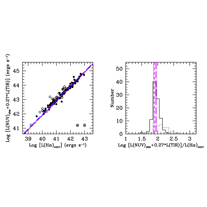
Figure 12: left panel: Combined NUV and TIR luminosities as a function of Balmer decrement ratio corrected H$\alpha$ luminosities for MK06 sample (solid circles) and SINGS sample (open circles). The error bars in the bottom-right corner denote median errors for the MK06 sample (right) and the SINGS sample (left). right panel: Histograms of the ratios of the TIR/NUV-corrected NUV luminosities to Balmer-corrected H$\alpha$ luminosities for MK06 sample (solid line) and SINGS sample (dotted line) in log scale. The color-coded lines represent the same model predictions as those in Figure 5.

Given that NUV emission can be from more evolved stars than FUV, we did not fit the corresponding coefficient $s_{\rm NUV}$ in eq. (13). Instead we estimated $s_{\rm NUV}$ from $s_{\rm FUV}$ according to $s_{\rm NUV}=s_{\rm FUV}-1$ (i.e.,$s_{\rm NUV}=2.83$). Then $a_{\rm NUV}$ was estimated from fitting eq. (13) with NUV substituted for FUV data and $s_{\rm NUV}$ fixed. The resulting fitted value of $a_{\rm NUV}$ was 0.27$\pm$0.02. Following the analyses for FUV, we compare the TIR/NUV corrected NUV luminosities with the Balmer-corrected H$\alpha$ luminosities in Figure 12. To our pleasant surprise, the combined NUV and TIR luminosities correlate with the Balmer-corrected H$\alpha$ luminosities nearly as well as FUV, and the scatter in NUV+TIR vs. L$({\rm H}\alpha)_{\rm corr}$ is almost the same as that in FUV+TIR vs. L$({\rm H}\alpha)_{\rm corr}$ (0.10 vs. 0.09 dex respectively). The average ratio of the TIR/NUV-corrected NUV luminosity to the Balmer-corrected H$\alpha$ luminosity is consistent with that expected for a constant star formation history over $\geq 1$ Gyr for a Kroupa IMF.

We also examined the trends of the residuals of the combined NUV and TIR luminosities relative to the Balmer decrement ratio corrected H$\alpha$ luminosities as functions of various parameters. We find that all the behaviors shown in NUV are similar to those in FUV. When 25$\micron$ infrared and radio continuum 1.4GHz luminosities are used as substitutes for TIR luminosities, we obtain coefficients $a_{\rm NUV}$ of 2.26$\pm$0.09 and $41.75\pm 2.97\times 10^{20}$ respectively. The scatters shown in NUV+25$\micron$ and NUV+1.4GHz versus L(H$\alpha$)_corr are identical to those shown in the same comparisons for FUV.

From the above analyses we can see that the NUV luminosity can serve as a rather good SFR indicator for our sample galaxies, and star formation activities have been going on smoothly in these galaxies over the last 1 Gyr. However, the use of NUV-based SFRs in galaxies with non-constant star formation histories during the last 1 Gyr may be problematic. Our experiment with the stellar population synthesis modelling code GALAXEV (Bruzual & Charlot 2003) shows that for a galaxy with a constant star formation history lasting for 100 Myr, the NUV emission at 300 Myr is 4.3% of its value at 100 Myr (compared to 2.6% for FUV). For a galaxy with high SFR ($\sim 23$ M_⊙ yr^-1) lasting for 100 Myr, the NUV emission at 300 Myr cannot be distinguished from a Milky Way like star-forming galaxy (with SFR $\sim 1$ M_⊙ yr^-1).

6 DISCUSSION

In previous sections we have derived prescriptions of using TIR/UV and FUV-NUV as UV dust attenuation indicators by employing a new empirical method. Specifically, these calibrations were obtained by fitting a TIR/UV versus FUV-NUV relation, which was defined by assuming that the UV attenuation estimated from TIR/UV ratio matches that from FUV-NUV color, to a nearby star-forming galaxy sample. We have demonstrated that the combinations of the observed FUV and NUV luminosities with the TIR luminosities (i.e., the TIR/UV corrected UV luminosities) are tightly correlated with the Balmer-corrected H$\alpha$ luminosities, and hence can serve as good SFR measures. By referencing to the TIR/UV corrected UV luminosities, we used the 25$\micron$ (or 24$\micron$) infrared or 1.4 GHz radio continuum luminosities as surrogate of the TIR luminosity to correct for the dust attenuation in the UV and found that they are slightly less accurate than the TIR luminosity. The combinations adopt the form of ${\rm L(UV)_{corr}=L(UV)_{obs}}+a\cdot{\rm L(\mbox{IR or radio})}$, and the corresponding attenuation in the UV has the form of ${\rm A_{UV}}=2.5\log[{1+{{a\cdot{\rm L(\mbox{\scriptsize IR or radio})}}\over{\rm L(UV)_{obs}}}}]$, where $a$ is the approximation of the product of the inverse of the bolometric correction $\eta_{\rm UV}$ and the factor ${(1-{\rm e}^{-{\tau_{\rm UV}}})}\over{(1-{\rm e}^{-\bar{\tau}})}$ (see Section 3). The coefficient $a$ and the dispersions of the combinations relative to the Balmer-corrected H$\alpha$ luminosities are listed in Table 3.

As we emphasized in Paper I, these composite indices have been calibrated over limited ranges of galaxy properties and physical environments. It is therefore important to understand the range of observations over which these calibrations are derived, and any systematics which were built into our calibrations. It is also useful to compare our results with the calibrations presented in the literature by different groups. We also reassess the consistency between the SFR derived from our dust attenuation corrected FUV luminosity and that based on Balmer-corrected H$\alpha$ luminosity.

6.1 Range of Applicability

In Paper I we have already discussed the ranges of the galaxy properties (e.g., the attenuation in H$\alpha$, TIR to H$\alpha$ flux ratio, ${\rm D_{n}}(4000{\rm\AA})$ and TIR luminosity) covered by our samples. Briefly our sample is composed of normal star-forming galaxies in the local universe. Neither early-type red galaxies nor dusty starburst galaxies are included in this sample, which is further demonstrated by the UV properties presented in this paper. The ranges of IRX and FUV-NUV color spanned by our sample galaxies are -0.19 to 2.39 dex and 0.07 to 1.06 mag respectively. This coverage in IRX and FUV-NUV color introduces uncertainties in the best fitted coefficients, as presented in Section 3, due to the lack of constraints from objects redder than 1.06 mag and bluer than 0.07 mag. As a result caution should be exercised when applying our calibrations to objects outside the above ranges (see Section 6.6).

6.2 Comparisons With Calibrations In The Literature

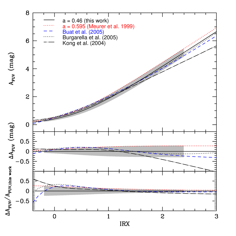
Figure 13: Comparison of the A_FUV vs. IRX (i.e., $\log{\rm[(L(TIR)/L(FUV)]}$ relation derived in this paper to those presented by others. The comparison is made in three different ways: the A_FUV itself (top), the difference in A_FUV relative to our calibration (middle) and the normalized difference (bottom) are plotted as a function of IRX. The solid line denotes our result. The shaded region indicates the uncertainty in our calibration over the range of IRX covered by our sample galaxies.

There exist several calibrations for normal star-forming galaxies in the literature. These calibrations were obtained under different assumptions about detailed star formation histories, dust attenuation curves, and the parameterization of the A_FUV – IRX relation (see below). It is thus necessary to test the consistency between them. We compare our calibration for IRX-based FUV attenuation estimates with those commonly used in the literature in Figure 13. Here the FUV attenuation (top panel), the residual of the FUV attenuation estimated using the calibrations given by other groups relative to that using our calibration (middle panel) and the normalized (percentage) residual (bottom panel) are plotted as a function of IRX. The black solid line denotes our calibration. The calibrations presented by other authors are shown with different line types as denoted in the top panel. Specifically, the commonly used calibrations for star-forming galaxies by Buat et al. (2005), Burgarella et al. (2005) and Kong et al. (2004) are plotted. We also show the well-known prescription for starburst galaxies by Meurer et al. (1999). The shaded region denotes the uncertainty in our calibration that is estimated using error propagation of eq. (15), without considering the measurement errors in FUV and TIR luminosities. The range of this region in IRX indicates the coverage by our sample objects, -0.19 to 2.39 dex (see Section 6.1). Outside this range the relation shown by the black solid line is simply the extrapolation of that defined by our data.

Before comparing the calibrations in the literature to our A_FUV – IRX relation, it is interesting to compare the published relations to each other first. From Figure 13, it can be clearly seen that over the whole range of IRX probed by our sample galaxies, the relations given by Buat et al. and Burgarella et al. are almost indistinguishable from each other – the difference is 0.1 mag at maximum. When compared to the Kong et al. relation, which is also derived for normal star-forming galaxies, at low IRX (L(TIR)$<10{\rm L(FUV)_{obs}}$), the three relations for star-forming galaxies stay close to each other – the difference is no more than 0.1 mag in the estimated attenuations. But at higher IRX (L(TIR)$>100{\rm L(FUV)_{obs}}$) the Kong et al. relation shows significant difference from the other two, 0.3-0.5 mag. Interestingly, the difference between the starbursts relation and the Buat et al. and Burgarella et al. relations is not dramatic (no more than 0.5 mag), given that they are derived for different types of galaxies. This comparison tells us for galaxies with $-0.19<$ IRX $<2.39$, when the attenuation prescriptions were used blindly, regardless of galaxy types, the uncertainty in the UV attenuation would be less than 0.5 mag.

Since our sample galaxies are mostly normal star-forming galaxies in the local universe (see Section 6.1), it is expected that our calibration is more similar to those calibrated for star-forming galaxies than for starbursts. Figure 13 confirms this expectation. The starburst curve obtained by Meurer et al. systematically overestimates the A_FUV compared to our calibration, although the difference is not dramatic, still within $1\sigma$ uncertainty of our calibration. The difference between starbursts and star-forming galaxies is expected because the mean age of the dust heating population should be systematically lower in starburst galaxies than in normal star-forming galaxies. Overall our calibration is very close to those for star-forming galaxies derived by Burgarella et al. and Buat et al. over the whole range of IRX spanned by our sample. It is worth noting that the prescriptions given by Burgarella et al. and Buat et al. are in polynomial forms, different from the form presented in eq. (2), which contributes to part of the differences. Among the three star-forming relations that we explored here, that of Kong et al. (2004) appears to deviate the most, as seen in Figure 13. At $0<{\rm IRX}<1.8$ the consistency between Kong et al. relation and ours is good, but at ${\rm IRX}<0$ and ${\rm IRX}>1.8$ the relation in Kong et al. over- and under-estimate ${\rm A_{FUV}}$ at $>1\sigma$ level, respectively.

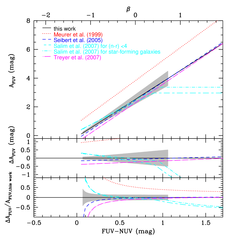
Figure 14: Top: Comparison of the A_FUV versus FUV-NUV relation obtained in this work to those presented by others. Middle: The difference in A_FUV between the relations given in the literature and that in this paper versus FUV-NUV. Bottom: The normalized residual versus FUV-NUV. The solid line denotes our result. The shaded region denotes the uncertainty in our calibration over the range of FUV-NUV color spanned by our sample galaxies.

We compare our calibration on A_FUV versus FUV-NUV relation with those in the literature in Figure 14. Similar to Figure 13, the A_FUV versus FUV-NUV relation is plotted in the top panel, the difference in A_FUV between the prescriptions in the literature and ours is shown in the middle panel, and the normalized (percentage) residual is shown in the bottom panel. The shaded region denotes the uncertainty in our calibration over the range of FUV-NUV color covered by our sample galaxies. As before the relation obtained in Section 3 is plotted with a black solid line and the calibrations presented by other authors are represented by different types of lines as denoted in the top panel. In this case, the relations plotted include the starburst galaxy calibration by Meurer et al. (1999), the calibrations for spectroscopically and NUV-r color selected star-forming galaxies by Salim et al. (2007), the relation by Treyer et al. (2007) for star-forming galaxies selected spectroscopically and the relation by Seibert et al. (2005) for a wide assortment of galaxy types.

It is obvious that at a given FUV-NUV color, the starburst line derived by Meurer et al. (1999) overestimates the A_FUV of normal star-forming galaxies dramatically compared to others. This is consistent with the well-known deviation of star-forming galaxies from starbursts in IRX-$\beta$ diagram (e.g., Kong et al. 2004; Cortese et al. 2006; Dale et al. 2007; Johnson et al. 2007b). The relations defined by star-forming galaxies stay close to each other but with different slopes and intercepts. Most of the differences shows up at FUV-NUV $<1$. For FUV-NUV $>1$, the relations converge except for those by Salim et al., which have constant A_FUV for galaxies redder than $0.90$ and $0.95$ in FUV-NUV color for NUV-r and spectroscopically selected galaxies respectively. As discussed in Section 4.3, the calibration derived by Treyer et al. (2007) underestimates the attenuation by 0.4 mag at FUV-NUV $\sim 0$ mag with the discrepancy decreasing as the object gets redder in FUV-NUV color. At FUV-NUV=1.7 mag, the Treyer et al. calibration gives consistent result with ours. The calibration by Seibert et al. (2005) is the most consistent one with ours, and the estimated A_FUV from their relation agrees with that from ours within $\pm 1\sigma$ for the range of FUV-NUV 0.2–1.7 mag. For bluer color (0 – 0.2 mag), the difference is a bit larger but always smaller than 0.2 mag in absolute scale. In terms of relative difference (bottom panel), both Treyer et al. and Seibert et al. relations are consistent with ours within $\pm 1\sigma$ at FUV-NUV $>$ 0.5, with increasing discrepancy at bluer color. For Salim et al. calibrations, both the absolute and the relative differences are large, far beyond $\pm 1\sigma$, for galaxies redder than $\sim 0.90$ in FUV-NUV because of the plateau in A_FUV defined in these relations, which is hard to be tested using our sample because of the limited range in FUV-NUV color covered by our galaxies (as indicated by the shaded region).

6.3 Comparison with Dust Attenuation Laws

As shown in Section 3, the scale parameter $s_{\rm FUV}$ in equation (9) represents the slope of the UV part of the attenuation curve. We derive $k_{\rm FUV}/k_{\rm NUV}$ from $s_{\rm FUV}$ and compare it with those derived from the commonly used dust attenuation laws published by Calzetti et al. (2000; originally from Calzetti et al. 1994;) and Charlot & Fall (2000). The attenuation curve by Calzetti et al. (1994) was obtained directly from the FUV-to-near-IR spectra of a sample of UV-selected starburst galaxies. Charlot & Fall (2000) used a similar but larger sample to derive their effective attenuation curve by tuning their model parameters to account for the distribution of the galaxies in the IRX, H$\alpha$/H$\beta$ ratio and EW(H$\alpha$) versus $\beta$ diagrams. The estimated values of $k_{\rm FUV}/k_{\rm NUV}$ from our calibration, Calzetti et al. (2000) and Charlot & Fall (2000) are 1.35$\pm 0.06$, 1.24 and 1.32, respectively, which means that in the UV part of the dust attenuation curve, the slope of the attenuation curve defined by our sample is consistent with that derived using Charlot & Fall (2000) attenuation law within the uncertainties but marginally steeper (at $\sim 2\sigma$ level) than that estimated from Calzetti et al. (1994;2000). The slope of our attenuation curve also suggests that the global FUV and NUV attenuations show no evidence for the effects of a strong 2175$\AA$ bump (e.g., O’Donnell 1994). For example, the O’Donnell Milky Way extinction curve has a $k_{\rm FUV}/k_{\rm NUV}$ ratio close to 0.9, which is much smaller than 1.35$\pm 0.06$ defined by our galaxies.

Based on the attenuation in the FUV estimated using our prescriptions, we can study the A_FUV – A_Hα relation. Figure 15 shows the IRX-derived (left panel) and FUV-NUV derived (right panel) A_FUV as a function of H$\alpha$/H$\beta$-derived A_Hα. The solid line in this figure is derived from eqs. (14) and (16), which present the relations between FUV-NUV color and A_Hα and A_FUV respectively. For comparison, the relation derived from Calzetti (2001) law after adapted to GALEX FUV waveband, which has the form ${\rm A_{FUV}}=1.82{\rm A_{H\alpha}}$, is plotted as the dotted line. As can be seen from the figure, at a given H$\alpha$ attenuation, Calzetti’s law gives a lower FUV attenuation estimate than ours and the difference becomes more significant for galaxies that are more attenuated. Quantitatively speaking, however, the slope of the solid line, which determined from our data, is 2.06$\pm$0.28, consistent with that given by Calzetti’s law within the error.

6.4 Comparisons Made For NUV

We performed similar comparisons for NUV with the calibrations published in the literature. When compared to the calibrations in the literature, similar to the results we saw for FUV, our calibration is in good agreement with the one given by Burgarella et al. (2005) within 0.1 mag for the whole range of Log[(TIR)/L(NUV)]. The A_NUV/A_Hα ratio defined by our data is 1.52$\pm$0.56, coincident with the predicted value from Calzetti (2001)’s law within the error.

6.5 Dust Heating From Old Stars

It is now well-known that a significant fraction of IR emission comes from dust heating by old stellar populations (e.g., Sauvage & Thuan 1992; Bell 2003 and references therein). In Paper I, by comparing our calibration for H$\alpha$+TIR as a SFR indicator with stellar population synthesis models, we found that for our sample objects up to 50% of the TIR emission could be from stars older than 100 Myr. Are the results presented here consistent with those estimates?

As mentioned in Section 3, the coefficient $a_{\rm FUV}$ in eq. (2) is the product of the inverse of the bolometric correction $\eta_{\rm FUV}$ and the factor ${(1-{\rm e}^{-\tau_{\rm FUV}})}\over{(1-{\rm e}^{-\overline{\tau}})}$. In Paper I, we have empirically derived $\bar{\tau}$ by combining the TIR luminosity and the multi-wavelength SEDs of a subset of MK06 galaxies with GALEX, SDSS and 2MASS observations. Briefly, eq. (6) was used to estimate $\bar{\tau}$ from the TIR and the bolometric luminosities, which were derived by adding the TIR luminosity to the integrated luminosity from the FUV to K band. After substituting the values of $\tau_{\rm FUV}$ and $\bar{\tau}$ into ${(1-{\rm e}^{-\tau_{\rm FUV}})}\over{(1-{\rm e}^{-\bar{\tau}})}$, we find that the median of ${(1-{\rm e}^{-\tau_{\rm FUV}})}\over{(1-{\rm e}^{-\bar{\tau}})}$ is around 1.5. Then the bolometric correction $1/\eta_{\rm FUV}$ is estimated to be $\sim 3.3$ by comparing $a_{\rm FUV}$ with ${(1-{\rm e}^{-\tau_{\rm FUV}})}\over{(1-{\rm e}^{-\bar{\tau}})}$.

In order to estimate the effect of dust heating from old stars, we compare the bolometric correction derived from our data to those from stellar population synthesis models. We found that the bolometric correction defined by our data is more than two times greater than the model prediction for a 100 Myr old stellar population with constant star formation history. This implies that stars older than 100 Myr must contribute to the dust heating. The spectral synthesis modelling using STARBURST99 indicates that the bolometric correction for a 10 Gyr old stellar population with constant star formation history, solar metallicity and either a Salpeter or a Kroupa IMF is only 15%–20% lower than the estimated value above. In other words, the mean property of our sample objects approximates a stellar population that has been constantly forming stars for 10 Gyr, which is exactly what we inferred from the analyses of H$\alpha$+TIR in Paper I. It is worth noting that the consistent inference drawn from Paper I and this paper ensure us the robustness of our results. However, this estimate of the average stellar population of our sample galaxies conflicts with the dust-free FUV-NUV color derived in Section 3, which is $\sim 0.04$ mag redder than a 10 Gyr old galaxy with constant star formation history. All the estimates made here are very rough and they should only be used as a guide to our understanding of the underlying physics shown by the data qualitatively. More careful modelling is needed for a quantitative understanding.

6.6 Systematic Uncertainties

As discussed in Section 6.1, our calibrations were derived over limited ranges of galaxy properties. So it is important to understand possible systematics which were built into our prescriptions.

First of all, prescriptions calibrated for different types of galaxies are different. This is not surprising because different types of galaxies show different IRX-$\beta$ (i.e., FUV-NUV color) relations. As shown in Section 6.2, the IRX-based and the FUV-NUV color-based attenuation correction prescriptions for star-forming galaxies differ from those for starburst galaxies. Another two extreme examples are dwarf irregulars and (Ultra)Luminous Infrared Galaxies ((U)LIRGs). Dale et al. (2009) examined the location of the Local Volume Legacy (LVL) sample galaxies in the IRX-$\beta$ diagram. Nearly two-thirds of LVL galaxies are dwarf/irregular systems. Those authors showed that the majority of LVL galaxies fall below the IRX-$\beta$ relation as defined by normal star-forming galaxies, and they cluster in an area with blue FUV-NUV color and low IRX (see also Lee et al. 2009). The range in IRX spanned by the LVL galaxies, for a given FUV-NUV color, is large – more than an order of magnitude. For (U)LIRGs, Howell et al. (2010; see also Goldader et al. 2002; Calzetti 2001) showed that (U)LIRGs in the Great Observatories ALL-sky LIRG Survey (GOALS) lie above the starburst relation, and the correlation between IRX and FUV-NUV color is not strong either. Similar to dwarf/irregulars, at a given FUV-NUV color, the (U)LIRGs span more than an order of magnitude in IRX. One assumption we made in our calibration method is that the attenuation derived from IRX matches that estimated from FUV-NUV color, which is reasonable for our normal star-forming galaxy sample given the relatively tight correlation between IRX and FUV-NUV color, as shown in Figure 3. However, it breaks down for dwarf irregulars and (Ultra)Luminous Infrared Galaxies given the large range of IRX spanned by these galaxies at a given FUV-NUV color. Therefore no attempt was made to calibrate an IRX-based and FUV-NUV color-based attenuation correction prescriptions for these galaxies.

Apart from different galaxy samples, the differences between different calibrations can be traced to the different methodologies. Previous calibrations have been based either on pure model assumptions, or on a comparison of observational data with models. The difference in the form of the parameterization of the prescriptions also contributes to the differences. As we can see from the comparisons in Section 6.2, the differences in methodology and parameterization (Buat et al. 2005; Burgarella et al. 2005 and this work) only account for a small portion of the differences, which cannot even be distinguished within $\pm 1\sigma$ uncertainty, and the main contributors to the different relations are the star formation history and the dust attenuation curve that includes the effect of the dust/star distribution, as suggested by other authors (e.g., Charlot & Fall 2000; Kong et al. 2004; Burgarella et al. 2005).

It is difficult to test the impact of dust attenuation curves on attenuation calibrations. However, it is possible to estimate the effect of dust-heating stellar populations. As discussed in Section 6.5, for our sample galaxies, up to half of the TIR emission could be from dust heated by stars older than 100 Myr. By contrast, in starburst galaxies, the dust is dominantly heated by stellar populations younger than 100 Myr (Meurer et al. 1999). This difference in dust-heating stellar populations of starbursts and our star-forming galaxies results in the difference in attenuation estimates, 0.3 mag at maximum over $-0.19<$ IRX $<2.39$, as shown in Figure 13. The effects on the UV color-based corrections are much larger than on IRX-based prescriptions. The IRX-based prescriptions are surprisingly consistent with each other. However different FUV-NUV based attenuation schemes have by comparison enormous inconsistencies. This underscores our concerns about color-based attenuation corrections based on scatter in our own data.

In principle, by comparing modelled SEDs with multi-wavelength data, the differences in star formation histories and dust attenuation curves can be taken into account on a galaxy-to-galaxy basis. However, the dust attenuations derived this way and the resulting relations of ${\rm A_{FUV}}$ versus IRX or ${\rm A_{FUV}}$ versus FUV-NUV color are dependent on the adopted stellar population synthesis models and the dust attenuation curves. On the other hand, the requirement of the availability of large libraries of models and multi-wavelength data makes this method less practical in many cases.

By contrast, our approach is more straightforward and less model-dependent. Our calibrations rely almost entirely on the data themselves and hence can serve as independent checks of other model-dependent methods. Although we assumed an average stellar population and dust attenuation curve (as discussed in Section 3), they do not introduce systematics into the calibrations and are valid on a statistical basis. Therefore, our calibrations should be robust. They also tend to be consistent with most of the published calibrations for normal star-forming galaxies.

The last possible systematic error comes from the TIR luminosities we adopted in our calibrations. We used TIR luminosities based on IRAS observations, which are systematically lower than those based on Spitzer/MIPS measurements by $24\%\pm 23\%$ on average (Section 2 and Figure 1 in Paper I). If we simply substitute the IRAS TIR luminosities by the MIPS TIR luminosities, the coefficient in front of IRX in eq. (15) will be lower by 24%, i.e., changes to 0.37, which is within the $1\sigma$ uncertainty of the coefficient. So if one uses MIPS TIR luminosities to estimate the FUV attenuation using our IRX-based prescription (i.e., eq. (15)), the uncertainty will be less than 0.3 mag.

In summary, our IRX-based attenuation correction has an uncertainty of $<0.3$ mag, when it is applied to starburst galaxies or to galaxies with MIPS based TIR luminosities. By contrast, if one uses our FUV-NUV color prescription to estimate the FUV attenuation for starbursts, he can underestimate the FUV attenuation by more than 1-2 mag. But for dwarf irregulars or (U)LIRGs, our prescriptions may suffer from severe problems.

6.7 The SFR Matching Method

In the introduction, we mentioned that Treyer et al. (2007) derived an A_FUV – FUV-NUV relation by matching the FUV-based and H$\alpha$-based SFRs. The attenuation derived this way is dependent on the intrinsic ratio of the FUV to H$\alpha$ luminosity, which in turn is dependent on model assumptions. Here we use a similar method to re-calibrate the A_FUV–IRX relation in order to evaluate the model dependence of the calibration obtained this way. We converted the Balmer-corrected H$\alpha$ luminosity to a Balmer-corrected FUV luminosity using a theoretical FUV/H$\alpha$ ratio and then force the combined observed (i.e., without internal dust attenuation correction) FUV and TIR luminosity to match the Balmer-corrected FUV luminosity so that the coefficient $a_{\rm FUV}$ in eq. (2) can be obtained. We used the same set of models as those used in Figure 5 and Figure 8. The model predictions and the best-fit coefficients $a_{\rm FUV}$ are listed in Table 2 (For reference the corresponding quantities for NUV are also listed.). Consistent with what we saw from Figure 5, Table 2 shows that our calibration derived in Section 3 is in excellent agreement with that predicted by assuming a constant star formation history with Kroupa IMF and age 100 Myr.

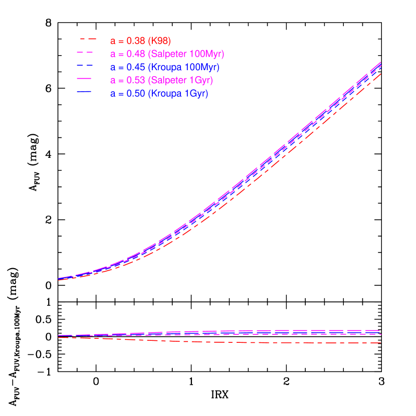
Figure 16: Top: A_FUV versus IRX (i.e., $\log{\rm[L(TIR)/L(FUV)]}$) relation with coefficient $a$ derived using the intrinsic FUV to H$\alpha$ luminosity ratio based on different stellar population assumptions, i.e., IMFs and ages (see text). $a$ is defined by ${\rm A_{FUV}}=2.5\log(1+a_{\rm FUV}\cdot 10^{\rm IRX})$ and is the approximation of the product of the inverse of the bolometric correction $\eta_{\rm FUV}$ and the factor ${(1-{\rm e}^{-{\tau_{\rm FUV}}})}\over{(1-{\rm e}^{-\bar{\tau}})}$. Bottom: The difference in A_FUV for different model assumptions.

The FUV/H$\alpha$ ratio changes at most by 10% when only the effect of a single parameter is taken into account, and accordingly the resulting coefficient $a_{\rm FUV}$ varies by 11%. The change in the coefficient directly affects the estimated attenuation from IRX. This impact is shown in Figure 16. It is clear that assuming a Salpeter or a Kroupa IMF does not affect the calibrations dramatically – at maximum $\sim$ 0.07 mag over the range of IRX=0 – 3. The calibrations are also affected by assuming either a 100 Myr old or a 1 Gyr (or older) old stellar population – at maximum $\sim$ 0.11 mag over the range tested. However the most widely used K98’s prescriptions give larger discrepancy – -0.2 mag at maximum when IRX=3. This large discrepancy with K98’s prescriptions is probably due to the use of the old stellar evolutionary models, which leads to an over-estimate of H$\alpha$ luminosity by 11% compared to that from STARBURST99 under the same set of assumptions of IMF, metallicity and star formation history.

From these tests, we can draw the following conclusions: (1) The calibration established using our new method is consistent with that based on SFR matching method for a constant star formation history with Kroupa IMF and age 100 Myr. (2) Compared to our prescription, the adoption of a Salpeter IMF and/or an older age both leads to an overestimate in A_FUV by up to 0.1 mag over the range of IRX=0 – 3. (3) Relative to our calibration, the widely used K98’s SFR prescriptions can underestimate A_FUV by up to 0.2 mag (at IRX=3).

7 SUMMARY

We have calibrated $\log{\rm[L(TIR)/L(FUV)_{obs}]}$ (i.e., IRX) and the FUV-NUV color as FUV dust attenuation indicators using a nearby star-forming galaxy sample studied by Moustakas & Kennicutt (2006). The combinations of 25$\micron$ and 1.4GHz radio continuum luminosities with the observed FUV luminosities were also empirically calibrated to probe the dust attenuation corrected FUV luminosities. Similar calibrations were derived for NUV band as well. The coefficients in these calibrations are summarized in Table 3 (see Section 6). These prescriptions provided in Table 3 can be used to derive attenuation-corrected star formation rates. Our main results can be summarized as follows.

1. The IRX-corrected FUV luminosities based on our new calibration, i.e.,

$${\rm L(FUV)_{corr}=L(FUV)_{obs}}+(0.46\pm 0.12){\rm L(\mbox{TIR})},$$

show tight and linear correlation with the Balmer decrement corrected H$\alpha$ luminosities, with a rms scatter of $\pm$0.09 dex ($\pm 0.23$ mag). Statistically speaking, their ratios are consistent with the model predictions from STARBURST99 by assuming a constant star formation rate over 100 Myr and solar metallicity. This consistency applies whether a Salpeter or a Kroupa IMF with lower and upper mass limits of 0.1 and 100 M_⊙ is adopted. Furthermore, these dust attenuation corrected FUV/H$\alpha$ ratios do not show any trend with other galactic properties over the ranges covered by our sample objects. These results suggest that linear combinations of TIR luminosities and the observed FUV luminosities (without internal attenuation corrections) are excellent star formation rate tracers.

2. The FUV-NUV corrected FUV luminosities are broadly correlated with the Balmer-corrected H$\alpha$ luminosities. But they do not trace each other linearly and the rms scatter is large – $\pm$0.23 dex ($\pm 0.58$ mag), which is $\sim 2.5$ times larger than the case for IRX-corrected FUV luminosities. In addition, the attenuation corrected FUV/H$\alpha$ ratios show correlations with a few other galactic properties, which will introduce systematic errors into the attenuation estimates in different galaxy samples. We confirm others’ findings that FUV-NUV color is not a good dust attenuation indicator for normal star forming galaxies though it can be used with caution when IR data are not available.

3. Linear combinations of 25$\micron$ and 1.4GHz radio continuum luminosities with the observed FUV luminosities can be used as surrogates of IRX-corrected FUV luminosities to trace the attenuation-corrected star formation rates. Their correlations with the Balmer-corrected H$\alpha$ luminosities are slightly less tight than the IRX-corrected FUV luminosities – 0.13 dex and 0.14 dex, and a non-linearity is shown in the correlation between FUV+1.4GHz and Balmer-corrected H$\alpha$ luminosities with a slope of $1.09\pm 0.02$.

4. Our calibrations are tested on normal star-forming galaxies with Balmer-based A_Hα = 0 – 2.5 mag, IRX = $-0.19$ – 2.39 and FUV-NUV = 0.07 – 1.06 mag. The A_FUV – IRX relation shows overall consistency with prescriptions for star-forming galaxies by Burgarella et al. (2005) and Buat et al. (2005) within $\pm 1\sigma$ uncertainty. While our A_FUV – FUV-NUV color relation is in good agreement with that presented by Seibert et al. (2005). When our IRX-based attenuation correction is applied to starburst galaxies or to galaxies with MIPS based TIR luminosities, it has an uncertainty of $<0.3$ mag. By contrast, if our FUV-NUV color prescription is used to estimate the FUV attenuation for starbursts, it can underestimate the FUV attenuation by more than 1-2 mag.

5. The estimated A_FUV using our prescriptions is related to the Balmer-based A_Hα in a way consistent with that given by Calzetti (2001)’s law within the error.

6. Our analyses show that the combination of the NUV and the TIR luminosities can serve as a rather good SFR indicator for our sample galaxies, but may become problematic in galaxies with non-constant star formation histories in the past $\sim 1$ Gyr.

Figure 1: Comparison of photometry from GALEX AIS images with that from images with longer exposure time for MK06 sample at FUV (left) and NUV (right) wavebands.

Figure 2: FUV-NUV color as a function of attenuation in H$\alpha$ line derived from the Balmer decrement ratio for MK06 sample (solid circles) and SINGS sample (open circles), with the corresponding UV continuum slope $\beta$ labelled on the right axis. The solid line is the bisector fitting to the MK06 sample. The error bars in the bottom-right corner denote median errors for the MK06 sample (right) and the SINGS sample (left).

Figure 3: IRX (i.e. $\log{\rm[L(TIR)/L(FUV)]}$) versus FUV-NUV color for the MK06 sample (solid circles) and the SINGS sample (open circles), with $\beta$ labelled on the top axis. The open squares with error bars represent the median, lower (25%) and upper (75%) quartiles in bins of width 0.2 mag in FUV-NUV color. The solid line, which has the form defined in eq. (13), is the best fit to the MK06 sample. The error bars in the bottom-right corner denote median errors for the MK06 sample (right) and the SINGS sample (left).

Figure 5: left panel: IRX-corrected FUV luminosities as a function of Balmer decrement ratio corrected H$\alpha$ luminosities for MK06 sample (solid circles) and SINGS sample (open circles). The lines overplotted represent the predicted relations by different SFR prescriptions (see text), which are the K98 prescription (red short-long dashed line) and models constructed using STARBURST99 by assuming a constant star formation history, solar metallicity for Kroupa IMF at 100 Myr (blue short dashed line), Kroupa IMF at 1 Gyr (blue long dashed line), Salpeter IMF at 100 Myr (magenta short dashed line) and Salpeter IMF at 1 Gyr (magenta long dashed line). The error bars in the bottom-right corner denote median errors for the MK06 sample (right) and the SINGS sample (left). right panel: Histograms of the ratios of the IRX-corrected FUV luminosities to Balmer-corrected H$\alpha$ luminosities for MK06 sample (solid line) and SINGS sample (dotted line) in log scale. The vertical lines represent the predicted values by different SFR prescriptions, as shown in left panel. This panel is given to show the differences between the models more clearly.

Figure 6: The logarithm residuals of the attenuation-corrected FUV luminosities from IRX relative to the Balmer-attenuation-corrected H$\alpha$ luminosities as functions of Balmer-attenuation-corrected H$\alpha$ luminosities (top-left panel), Balmer-attenuation-corrected H$\alpha$ luminosities per unit area (top-right panel), attenuation in H$\alpha$ calculated from H$\alpha$/H$\beta$ ratio (bottom-left) and axial ratio (inclination) b/a (bottom-right). The label at the top of the top-left panel shows the corresponding SFR according to the L(H$\alpha$) – SFR relation given by K98. The solid circles represent MK06 galaxies while the open circles denote SINGS galaxies. The dashed line denotes the predicted value by the STARBURST99 synthesis model for a constant star formation history, solar metallicity and Kroupa IMF at 100 Myr.

Figure 7: Similar to Figure 6 but with residuals plotted as functions of integrated Equivalent Width at H$\alpha$ (top-left panel), 4000$\AA$ break (D${}_{\rm n}(4000\AA)$) (top-right panel), gas-phase oxygen abundance (12+log(O/H)) (bottom-left panel) and FIR color ($f_{\nu}(60\micron)/f_{\nu}(100\micron)$) (bottom-right panel). See Figure 6 for the explanation of the symbols.

Figure 9: The logarithm residuals of the attenuation-corrected FUV luminosities from FUV-NUV color relative to the Balmer-attenuation-corrected H$\alpha$ luminosities as functions of Balmer-attenuation-corrected H$\alpha$ luminosities (top-left panel), Balmer-attenuation-corrected H$\alpha$ luminosities per unit area (top-right panel), attenuation in H$\alpha$ calculated from H$\alpha$/H$\beta$ ratio (bottom-left) and axial ratio (inclination) b/a (bottom-right). The label at the top of the top-left panel shows the corresponding SFR according to the L(H$\alpha$) – SFR relation given by K98. The solid circles represent MK06 galaxies while the open circles denote SINGS galaxies. The dashed line denotes the predicted value by the STARBURST99 synthesis model for a constant star formation history, solar metallicity and Kroupa IMF at 100 Myr.

Figure 10: Similar to Figure 9 but with residuals plotted as functions of integrated Equivalent Width at H$\alpha$ (top-left panel), 4000$\AA$ break (D${}_{\rm n}(4000\AA)$) (top-right panel), gas-phase oxygen abundance (12+log(O/H)) (bottom-left panel) and FIR color ($f_{\nu}(60\micron)/f_{\nu}(100\micron)$) (bottom-right panel). See Figure 9 for the explanation of the symbols.

Figure 11: Linear combinations of the observed FUV luminosities with 25$\micron$ luminosities (left panel) and 1.4GHz luminosities (right panel) compared to the Balmer-corrected H$\alpha$ luminosities, with the scaling coefficient derived by matching the combined FUV and 25$\micron$ or 1.4GHz luminosities with the IRX-corrected FUV luminosities. The solid circles represent MK06 galaxies, the open circles denote SINGS galaxies with the integrated measurements while the open squares denote the central 20″ $\times$ 20″ regions of SINGS galaxies. The dashed line denotes the predicted value by the STARBURST99 synthesis model for a constant star formation history, solar metallicity and Kroupa IMF at age 100 Myr. The error bars in the bottom-right corner denote median errors for the MK06 sample (right) and the SINGS sample (left).

Figure 15: IRX (left panel) and FUV-NUV (right panel) derived dust attenuation in FUV as a function of the dust attenuation in H$\alpha$ line. The solid line represents the relation defined by our sample galaxies and the dotted line denotes that given by Calzetti (2001), with the difference in E(B-V)_⋆ and E(B-V)_gas taken into account and adapted to GALEX FUV waveband. The error bars in the bottom-right corner denote median errors for the MK06 sample (right) and the SINGS sample (left).

Table 1: GALEX UV photometry for MK06 sample

Name	Distance	FUV	NUV
	(Mpc)	(mJy)	(mJy)
ARP256	113.9	2.83$\pm$0.13	3.93$\pm$0.11
NGC0157	24.0	13.66$\pm$0.63	22.41$\pm$0.62
NGC0245	56.5	4.08$\pm$0.23	6.34$\pm$0.22
IC0051	24.8	1.16$\pm$0.11	1.99$\pm$0.13
NGC0337	23.5	11.22$\pm$0.52	19.54$\pm$0.54
IC1623	84.1	6.00$\pm$0.28	7.81$\pm$0.22
MCG-03-04-014	139.9	0.23$\pm$0.01	0.52$\pm$0.01
NGC0695	135.4	0.65$\pm$0.03	1.40$\pm$0.04
NGC0877	54.6	5.11$\pm$0.47	7.56$\pm$0.40
NGC0922	43.4	14.21$\pm$0.66	16.39$\pm$0.45
NGC0958	79.5	1.50$\pm$0.07	2.46$\pm$0.07
NGC0959	10.9	4.52$\pm$0.21	6.51$\pm$0.18
NGC0976	59.8	1.97$\pm$0.28	3.20$\pm$0.25
NGC1058	9.8	5.88$\pm$0.42	9.91$\pm$0.39
NGC1084	20.0	13.77$\pm$0.64	22.52$\pm$0.62
NGC1140	21.2	9.78$\pm$0.45	11.76$\pm$0.33
NGC1156	7.8	24.71$\pm$1.14	30.49$\pm$0.84
NGC1359	28.0	11.54$\pm$0.58	13.78$\pm$0.42
NGC1385	21.2	17.90$\pm$0.83	24.76$\pm$0.69
IRAS03359+1523	147.8	0.71$\pm$0.36	1.25$\pm$0.27
NGC1421	29.7	9.69$\pm$0.66	14.88$\pm$0.54
UGC02982	74.5	0.63$\pm$2.78	0.95$\pm$1.90
NGC1569	2.0	372.46$\pm$17.16	671.21$\pm$18.62
NGC2139	26.7	13.88$\pm$0.72	20.28$\pm$0.61
NGC2337	7.9	4.84$\pm$0.31	6.27$\pm$0.25
NGC2415	57.2	5.53$\pm$0.29	9.41$\pm$0.29
NGC2500	11.0	13.39$\pm$0.62	15.17$\pm$0.42
NGC2537	6.9	9.07$\pm$0.42	10.77$\pm$0.30
UGC05028	56.7	1.62$\pm$0.08	2.45$\pm$0.07
NGC2903	8.9	34.67$\pm$1.60	60.86$\pm$1.68
NGC3239	10.5	14.91$\pm$0.69	26.41$\pm$0.73
NGC3265	25.0	0.59$\pm$0.03	0.97$\pm$0.03
UGC05720	26.9	4.05$\pm$0.19	5.05$\pm$0.14
NGC3344	7.9	35.41$\pm$1.63	49.66$\pm$1.37
NGC3353	19.1	4.95$\pm$0.23	6.10$\pm$0.17
NGC3367	49.3	10.21$\pm$0.52	15.56$\pm$0.47
ARP270	30.3	17.38$\pm$0.80	22.15$\pm$0.61
NGC3432	10.4	15.66$\pm$0.75	22.68$\pm$0.66
NGC3442	31.6	2.91$\pm$0.15	3.94$\pm$0.13
NGC3521	8.6	17.09$\pm$0.79	34.79$\pm$0.96
NGC3600	13.3	2.44$\pm$0.11	3.54$\pm$0.10
IC0691	23.7	1.17$\pm$0.08	1.58$\pm$0.07
NGC3726	19.8	20.25$\pm$0.99	28.26$\pm$0.83
NGC3738	4.9	11.49$\pm$0.56	13.85$\pm$0.40
NGC3769	19.8	3.98$\pm$0.23	5.89$\pm$0.21
UGC06665	87.4	2.46$\pm$0.11	3.41$\pm$0.10
NGC3870	19.8	3.33$\pm$0.18	4.02$\pm$0.13
NGC3893	15.5	13.80$\pm$0.69	25.50$\pm$0.74
NGC3928	16.9	2.47$\pm$0.15	3.72$\pm$0.14
NGC3949	19.8	13.60$\pm$0.66	20.83$\pm$0.60
NGC4004	55.6	2.49$\pm$0.12	3.61$\pm$0.10
ARP244	25.0	33.06$\pm$1.52	46.56$\pm$1.29
NGC4051	15.5	15.22$\pm$0.76	23.94$\pm$0.72
NGC4062	11.4	3.96$\pm$0.20	7.13$\pm$0.20
NGC4085	19.8	1.40$\pm$0.12	2.70$\pm$0.13
NGC4088	19.8	11.37$\pm$0.60	18.43$\pm$0.58
NGC4096	10.8	8.04$\pm$0.37	12.58$\pm$0.35
NGC4100	19.8	4.24$\pm$0.31	8.24$\pm$0.32
NGC4214	2.9	52.74$\pm$2.44	64.17$\pm$1.78
NGC4218	19.8	3.26$\pm$0.16	4.05$\pm$0.12
NGC4254	12.9	31.13$\pm$1.46	56.30$\pm$1.57
NGC4303	10.6	43.55$\pm$2.01	62.09$\pm$1.72
NGC4384	42.8	1.99$\pm$0.13	3.06$\pm$0.12
NGC4414	17.7	7.46$\pm$0.35	14.08$\pm$0.39
NGC4605	5.2	21.53$\pm$0.99	31.48$\pm$0.87
NGC4618	8.9	23.61$\pm$1.09	30.54$\pm$0.84
NGC4625	10.2	3.88$\pm$0.18	5.25$\pm$0.14
NGC4651	20.6	9.52$\pm$0.44	13.98$\pm$0.39
NGC4656	8.7	44.27$\pm$2.04	48.63$\pm$1.34
NGC4666	27.6	6.14$\pm$0.35	9.15$\pm$0.34
NGC4670	23.2	7.82$\pm$0.37	9.38$\pm$0.26
NGC4713	13.7	13.05$\pm$0.61	17.91$\pm$0.50
NGC4900	9.0	9.86$\pm$0.47	15.42$\pm$0.43
NGC5014	23.8	0.86$\pm$0.05	1.55$\pm$0.05
MRK0066	95.6	1.36$\pm$0.09	1.60$\pm$0.06
NGC5194	8.0	123.02$\pm$5.67	196.70$\pm$5.43
ARP240	104.9	4.11$\pm$0.25	6.70$\pm$0.26
NGC5253	3.1	41.14$\pm$1.90	54.93$\pm$1.52
NGC5430	49.0	2.57$\pm$0.16	4.05$\pm$0.14
NGC5607	112.2	1.34$\pm$0.11	2.46$\pm$0.10
NGC5591	117.6	0.68$\pm$0.07	1.28$\pm$0.08
NGC5653	58.7	1.56$\pm$0.11	3.02$\pm$0.11
NGC5676	37.7	3.92$\pm$0.31	8.09$\pm$0.31
UGC09560	23.7	3.30$\pm$0.15	3.52$\pm$0.10
IC1076	94.6	0.88$\pm$0.10	1.54$\pm$0.09
NGC5996	54.6	5.63$\pm$0.26	7.93$\pm$0.22
NGC6052	74.8	4.99$\pm$0.30	7.60$\pm$0.24
NGC6090	130.2	1.15$\pm$0.05	1.99$\pm$0.05
NGC6926	87.6	3.08$\pm$0.54	5.34$\pm$0.45
IC5179	50.3	3.01$\pm$0.18	5.52$\pm$0.20
NGC7316	79.0	2.58$\pm$0.13	3.95$\pm$0.11
CGCG453-062	106.0	0.13$\pm$0.02	0.35$\pm$0.02
NGC7624	61.1	0.80$\pm$0.05	2.04$\pm$0.06
NGC7625	24.4	1.18$\pm$0.06	2.78$\pm$0.08
NGC7673	48.9	5.96$\pm$0.28	7.70$\pm$0.21
NGC7678	49.7	4.87$\pm$0.23	7.25$\pm$0.20
NGC7798	34.6	3.65$\pm$0.17	5.59$\pm$0.16

Table 2:

Model description	$\log C_{FUV}$	$\log C_{NUV}$	$\log C_{H\alpha}$	$C_{FUV}/C_{H\alpha}$	$C_{NUV}/C_{H\alpha}$	$a_{FUV}$	$a_{NUV}$
K98	-43.147	-42.975	-41.102	0.0090	0.0134	0.38	0.21
Salpeter IMF, ${\rm Z}_{\odot}$, 100 Myr	-43.170	-42.959	-41.056	0.0077	0.0125	0.48	0.24
Kroupa IMF, ${\rm Z}_{\odot}$, 100 Myr	-43.350	-43.137	-41.257	0.0081	0.0132	0.45	0.22
Salpeter IMF, ${\rm Z}_{\odot}$, 1 Gyr	-43.207	-43.023	-41.056	0.0071	0.0108	0.53	0.30
Kroupa IMF, ${\rm Z}_{\odot}$, 1 Gyr	-43.384	-43.196	-41.257	0.0075	0.0115	0.50	0.27

Table 3: Summary of Coefficients

Relation	Coefficient	Dispersion
L(FUV)obs + a*L(TIR)	0.46$\pm$0.120	0.09
L(FUV)obs + a*L(25 $\mu$m)	3.89$\pm$0.150	0.13
L(FUV)obs + a*L1.4GHz	71.81$\pm$5.06 $\times$ 1.E20	0.14
L(NUV)obs + a*L(TIR)	0.27$\pm$0.02	0.10
L(NUV)obs + a*L(25 $\mu$m)	2.26$\pm$0.09	0.13
L(NUV)obs + a*L1.4GHz	41.75$\pm$2.97 $\times$ 1.E20	0.14

References

- (1) Balogh, M. L., Morris, S. L., Yee, H. K. C., Carlberg, R. G., & Ellingson, E. 1999, ApJ, 527, 54
- (2) Bell, E. F. 2002, ApJ, 577, 150
- (3) Bell, E.F. 2003, ApJ, 586, 794
- (4) Bell, E. F., & Kennicutt, R. C., Jr. 2001, ApJ, 548, 681
- (5) Boissier, S., et al. 2007, ApJS, 173, 524
- (6) Boquien, M., et al. 2009, ApJ, 706, 553
- (7) Brinchmann, J., Charlot, S., White, S. D. M., Tremonti, C., Kauffmann, G., Heckman, T., & Brinkmann, J. 2004, MNRAS, 351, 1151
- (8) Bruzual, G. 1983, ApJ, 273, 106
- (9) Bruzual, G., & Charlot, S. 2003, MNRAS, 344, 1000
- (10) Buat, V., Boselli, A., Gavazzi, G., & Bonfanti, C. 2002, A&A, 383, 801
- (11) Buat, V., Donas, J., Milliard, B., & Xu, C. 1999, A&A, 352, 371
- (12) Buat, V. et al. 2010, MNRAS, 409, 1
- (13) Buat, V. et al. 2005, ApJ, 619, L51
- (14) Buat, V., & Xu, C. 1996, A&A, 306, 61
- (15) Burgarella, D., Buat, V., & Iglesias-Páramo, J. 2005, MNRAS, 360, 1413
- (16) Calzetti, D. 1997, AJ, 113, 162
- (17) Calzetti, D. 2001, PASP, 113, 1449
- (18) Calzetti, D., Armus, L., Bohlin, R. C., Kinney, A. L., Koornneef, J., & Storchi-Bergmann, T. 2000, ApJ, 533, 682
- (19) Calzetti, D., et al. 2005, ApJ, 633, 871
- (20) Calzetti, D., et al. 2010, ApJ, 714, 1256
- (21) Calzetti, D., Kinney, A. L., & Storchi-Bergmann, T. 1994, ApJ, 429, 582
- (22) Cardelli, J. A., Clayton, G. C., & Mathis, J. S. 1989, ApJ, 345, 245
- (23) Charlot, S., & Fall, S. M. 2000, ApJ, 539, 718
- (24) Cortese, L., et al. 2006, ApJ, 637, 242
- (25) Cortese, L., Boselli, A., Franzetti, P., Decarli, R., Gavazzi, G., Boissier, S., & Buat, V. 2008, MNRAS, 386, 1157
- (26) Dale, D. A., & Helou, G. 2002, ApJ, 576, 159
- (27) Dale, D.A., et al. 2007, ApJ, 655, 863
- (28) Dale, D.A., et al. 2009, ApJ, 703, 517
- (29) Feigelson, E. D., & Babu, G. J. 1992, ApJ, 397, 55
- (30) Gil de Paz, A., et al. 2007, ApJS, 173, 185
- (31) Gordon, K.D., Clayton, G.C., Witt, A.N., & Misselt, K.A. 2000, ApJ, 533, 236
- (32) Granato, G. L., Lacey, C. G., Silva, L., Bressan, A., Baugh, C. M., Cole, S., & Frenk, C. S. 2000, ApJ, 542, 710
- (33) Goldader, J. D., Meurer, G., Heckman, T. M., Seibert, M., Sanders, D. B., Calzetti, D., & Steidel, C. C. 2002, ApJ, 568, 651
- (34) Heckman, T. M., Robert, C., Leitherer, C., Garnett, D. R., & van der Rydt, F. 1998, ApJ, 503, 646
- (35) Howell, J. H., et al. 2010, ApJ, 715, 572
- (36) Iglesias-Páramo, J., et al. 2006, ApJS, 164, 38
- (37) Isobe, T., Feigelson, E. D., Akritas, M. G., & Babu, G. J. 1990, ApJ, 364, 104
- (38) Johnson, B.D., et al. 2007a, ApJS, 173, 377
- (39) Johnson, B.D., et al. 2007b, ApJS, 173, 392
- (40) Kauffmann, G., et al. 2003, MNRAS, 341, 33
- (41) Kennicutt, R.C. 1998, ARA&A, 36, 189
- (42) Kennicutt, R. C., Tamblyn, P., & Congdon, C. W. 1994, ApJ, 435, 22
- (43) Kennicutt, R.C., et al. 2003, PASP, 115, 98
- (44) Kennicutt, R.C., et al. 2009, ApJ, 703, 1672
- (45) Kewley, L. J., Heisler, C. A., Dopita, M. A., & Lumsden, S. 2001, ApJS, 132, 37
- (46) Kinney, A.L., Bohlin, R. C., Calzetti, D., Panagia, N., & Wyse, R. F. G. 1993,ApJS, 86, 5
- (47) Kong, X., Charlot, S., Brinchmann, J., & Fall, S.M. 2004, MNRAS, 349, 769
- (48) Kroupa, P., & Weidner, C. 2003, ApJ, 598, 1076
- (49) Lee, J. C., et al. 2009, ApJ, 706, 599
- (50) Leitherer, C., & Heckman, T. M. 1995, ApJS, 96, 9
- (51) Leitherer, C., et al. 1999, ApJS, 123, 3
- (52) Li, A., & Draine, B. T. 2001, ApJ, 554, 778
- (53) Martin, D. C., et al. 2005, ApJ, 619, L1
- (54) Madau, P., Pozzetti, L., & Dickinson, M. 1998, ApJ, 498, 106
- (55) Meurer, G. R., Heckman, T. M., & Calzetti, D. 1999, ApJ, 521, 64
- (56) Meurer, G. R., Heckman, T. M., Leitherer, C., Kinney, A., Robert, C., & Garnett, D. R. 1995, AJ, 110, 2665
- (57) Meurer, G. R., et al. 2009, ApJ, 695, 765
- (58) Morrissey, P., et al. 2007, ApJS, 173, 682
- (59) Moustakas, J., & Kennicutt, R.C. 2006, ApJS, 164, 81 (MK06)
- (60) Moustakas, J., Kennicutt, R.C., & Tremonti, C.A. 2006, ApJ, 642, 775
- (61) O’Donnell, J.E. 1994, ApJ, 422, 158
- (62) Panuzzo, P., Granato, G. L., Buat, V., Inoue, A. K., Silva, L., Iglesias-Páramo, J., & Bressan, A. 2007, MNRAS, 375, 640
- (63) Salim, S., et al. 2009, ApJ, 700, 161
- (64) Salim, S., et al. 2007, ApJS, 173, 267
- (65) Salpeter, E.E. 1955, ApJ, 121, 161
- (66) Sauvage, M., & Thuan, T.X. 1992, ApJ, 396, 69
- (67) Schlegel, D. J., Finkbeiner, D. P., & Davis, M. 1998, ApJ, 500, 525
- (68) Seibert, M., et al. 2005, ApJ, 619, 55
- (69) Takeuchi, T. T., Buat, V., Heinis, S., Giovannoli, E., Yuan, F.-T., Iglesias-Páramo, J., Murata, K. L., & Burgarella, D. 2010, A&A, 514, 4
- (70) Treyer, M., et al. 2007, ApJS, 173, 256
- (71) Vázquez, G. A., & Leitherer, C. 2005, ApJ, 621, 695
- (72) Wang, B., & Heckman, T. M. 1996, ApJ, 457, 645
- (73) Witt, A. N., & Gordon, K. D. 2000, ApJ, 528, 799
- (74) Witt, A. N., Thronson, H. A., Jr., & Capuano, J. M., Jr. 1992, ApJ, 393, 611
- (75) Zhu, Y. N., Wu, H., Cao, C., & Li, H. N. 2008, ApJ, 686, 155