Resonant suppression of thermal stability of the nanoparticle magnetization by a rotating magnetic field

Abstract

We study the thermal stability of the periodic (P) and quasi-periodic (Q) precessional modes of the nanoparticle magnetic moment induced by a rotating magnetic field. An analytical method for determining the lifetime of the P mode in the case of high anisotropy barrier and small amplitudes of the rotating field is developed within the Fokker-Planck formalism. In general case, the thermal stability of both P and Q modes is investigated by numerical simulation of the stochastic Landau-Lifshitz equation. We show analytically and numerically that the lifetime is a nonmonotonic function of the rotating field frequency which, depending on the direction of field rotation, has either a pronounced maximum or a deep minimum near the Larmor frequency.

I INTRODUCTION

Magnetic nanoparticles are of great interest because of their nanoscale physical properties and many current and potential applications. These applications range from high-density storage mediaMTMA ; Ross and spintronic devicesZFS ; WABD to biomedical applications like drug delivery, cell separation, cancer treatment and many others (for a review, see Refs. LFPR, ; Ferr, ; PCJD, ). Since the physical properties of nanoparticles play a decisive role in all these applications, their study is of fundamental importance. In particular, for high-density storage media, e.g., bit-patterned mediaRoss ; Richt where each nanoparticle is a carrier of information, the thermal stability of a given direction (or magnitude) of the nanoparticle magnetic moment is one of the most important problems. The reason is that under thermal fluctuations the magnetic moment can be randomly switched to a new state leading to the loss of information.

In the case of ferromagnetic nanoparticles, the fluctuation dynamics of the nanoparticle magnetic moment can be described by the stochastic Landau-Lifshitz equation. If the noise term in this equation is approximated by the Gaussian white noise, then the probability density of the magnetic moment satisfies the Fokker-Planck equation whose properties are well known.Ris This approach, introduced by BrownBrown almost five decades ago, has become an important tool in the study of stochastic magnetic dynamics (see Ref. CKW, and references therein). To characterize the thermal stability in the case of uniaxial nanoparticles, it is often enough to determine the lifetimes of the nanoparticle magnetic moment in the “up” and “down” states. In the above approach, the lifetime in a given state is usually interpreted as the relaxation time. However, from a theoretical point of view, the lifetime is reasonable to associate with the mean first-passage time (MFPT), i.e., average time that a random process dwells in a prescribed state. An additional advantageous feature of this definition of the lifetime is that the MFPT method is mathematically well developed.HTB ; Gar ; Red This approach was first applied to study the magnetic relaxation in systems of noninteractingDY and dipolar interactingDLT nanoparticles subjected to a constant magnetic field.

In general, the lifetime depends on both intrinsic properties of nanoparticles and external magnetic fields. The case when the external fields contain a rotating magnetic field applied perpendicular to the easy axes of nanoparticles has a particular interest. On the one hand, this is because the rotating field plays a key role in the microwave-assisted switchingTWM ; SW1 ; SW2 ; PH ; WB ; ZZT and, on the other hand, because the corresponding dynamical equations (without accounting the thermal fluctuations) can often be solved analytically.BSM ; BMS1 ; DLHT ; BMSAB ; CSS Specifically, it has been shownBSM (see also Ref. BMS, ) that the rotating field can induce two types of the stable precessional modes of the magnetic moment, namely, the periodic (P) and quasi-periodic (Q) modes. Under certain conditions,DLBH ; LPRB one mode can exist in the up state of the magnetic moment and the other in the down state. The thermal fluctuations make the random transitions between these modes possible, and the problem of the lifetime of the P and Q modes appears. Some aspects of this problem have already been considered previously in the context of magnetic relaxation and induced magnetization.DLH ; DSTH1 ; DSTH2 But the dependence of the lifetime on the parameters of the rotating field has not been studied systematically. At the same time, the effect of strong dependence of the lifetime on the rotating field frequency, which is expected to exist in the vicinity of the Larmor frequency, could be important for applications. Therefore, in this paper we present a detailed analytical and numerical analysis of the above mentioned problem.

The paper is organized as follows. In Sec. II, we describe the model and define the lifetime of both the P and Q modes. Here we also derive the boundary conditions and transformation properties of the lifetime. In Sec. III, we develop an analytical method for calculating the frequency dependence of the lifetime of the P mode in the case of high anisotropy barrier. Our numerical results obtained by the simulation of the deterministic and stochastic Landau-Lifshitz equations are presented in Sec. IV. Specifically, the features of the P and Q modes at zero temperature are studied in Sec. IV.1 and the effects of thermal fluctuations are considered in Sec. IV.2. Finally, in Sec. V we summarize our findings.

II LIFETIMES OF THE PRECESSIONAL MODES

II.1 Basic equations of the model

To study the influence of the rotating magnetic field on the thermal stability of the nanoparticle magnetization, we use a minimal model with coherent spin dynamics. Within this model, which is applicable to particles whose exchange energy is comparatively large, the magnetic state of each particle is completely characterized by the magnetic moment $\mathbf{m}=\mathbf{m}(t)$ of a fixed magnitude $m=|\mathbf{m}|$. Due to its interaction with a heat bath, $\mathbf{m}(t)$ is a vector random process which can be described by the stochastic Landau-Lifshitz equationKH

$$\frac{d}{dt}\mathbf{m}=-\gamma\mathbf{m}\times(\mathbf{H}+\mathbf{n})-\frac{\lambda\gamma}{m}\,\mathbf{m}\times(\mathbf{m}\times\mathbf{H}),$$ (1)

where $\gamma(>0)$ is the gyromagnetic ratio, $\lambda(>0)$ is the damping parameter, the cross denotes the vector product, and $\mathbf{H}=\mathbf{H}(t)$ and $\mathbf{n}=\mathbf{n}(t)$ are the effective magnetic fields. The first field is given by $\mathbf{H}=-\partial W/\partial\mathbf{m}$, where $W$ is the magnetic energy of the particle which, in the case under consideration, contains only the uniaxial anisotropy energy $(1/2)H_{a}m(1-m_{z}^{2}/m^{2})$ and the Zeeman energy $-\mathbf{m}\cdot\mathbf{h}(t)$, i.e., $\mathbf{H}=H_{a}(m_{z}/m)\mathbf{e}_{z}+\mathbf{h}(t)$. Here, the $z$-axis of a Cartesian coordinate system $xyz$ with unit vectors $\mathbf{e}_{x}$, $\mathbf{e}_{y}$ and $\mathbf{e}_{z}$ is chosen to be parallel to the easy axis of magnetization, $H_{a}(>0)$ is the anisotropy field, $m_{z}=\mathbf{m}\cdot\mathbf{e}_{z}$, the dot denotes the scalar product, and $\mathbf{h}(t)$ is the rotating magnetic field. We assume that $\mathbf{h}(t)$ is applied perpendicular to the $z$-axis, so that

$$\mathbf{h}(t)=h\cos(\omega t)\mathbf{e}_{x}+\rho h\sin(\omega t)\mathbf{e}_{y},$$ (2)

where $h=|\mathbf{h}(t)|$ is the field amplitude, $\omega$ is the angular rotation frequency, and $\rho=-1$ (for clockwise rotation) or $+1$ (for counterclockwise rotation). It is this field that induces the precessional modes of $\mathbf{m}(t)$.

The effective field $\mathbf{n}(t)$ accounts for the thermal fluctuations. It is assumed that the Cartesian components $n_{\alpha}(t)$ $(\alpha=x,y,z)$ of $\mathbf{n}(t)$ are independent Gaussian white noises with zero means and correlation functions $\langle n_{\alpha}(t_{1})n_{\alpha}(t_{2})\rangle=2\Delta\delta(t_{2}-t_{1})$. Here, the angular brackets denote averaging over all realizations of $\mathbf{n}(t)$, $\Delta=\lambda k_{B}T/\gamma m$ is the noise intensity, $k_{B}$ is the Boltzmann constant, $T$ is the absolute temperature, and $\delta(t)$ is the Dirac $\delta$ function. In accordance with this definition of $\mathbf{n}(t)$, the random process $\mathbf{m}(t)$ is Markovian and can be described within the Fokker-Planck formalism.

Because Eq. (1) preserves the length of the magnetic moment $\mathbf{m}(t)$, it is convenient to write the Fokker-Planck equation that corresponds to Eq. (1) in spherical coordinates. Introducing the polar and azimuthal angles $\theta(t)$ and $\varphi(t)$ of $\mathbf{m}(t)$, the forward and backward Fokker-Planck equations for the conditional probability density $P=P(\theta,\psi,\tilde{t}|\theta^{\prime},\psi^{\prime},\tilde{t}^{\prime})$ ($\tilde{t}\geq\tilde{t}^{\prime}$) can be written asDSTH1 ; DSTH2

$$\displaystyle\frac{\partial^{2}P}{\partial\theta^{2}}+\frac{1}{\sin^{2}\theta}\frac{\partial^{2}P}{\partial\psi^{2}}-\frac{\partial}{\partial\theta}\bigg{(}\cot\theta+\frac{2a}{\lambda}u(\theta,\psi)\bigg{)}P$$

$$\displaystyle-\frac{2a}{\lambda}\frac{\partial}{\partial\psi}[v(\theta,\psi)-\rho\tilde{\omega}]P=\frac{2a}{\lambda}\frac{\partial P}{\partial\tilde{t}}$$ (3)

and

$$\displaystyle\frac{\partial^{2}P}{\partial\theta^{\prime 2}}+\frac{1}{\sin^{2}\theta^{\prime}}\frac{\partial^{2}P}{\partial\psi^{\prime 2}}+\bigg{(}\cot\theta^{\prime}+\frac{2a}{\lambda}u(\theta^{\prime},\psi^{\prime})\bigg{)}\frac{\partial P}{\partial\theta^{\prime}}$$

$$\displaystyle+\frac{2a}{\lambda}[v(\theta^{\prime},\psi^{\prime})-\rho\tilde{\omega}]\frac{\partial P}{\partial\psi^{\prime}}=-\frac{2a}{\lambda}\frac{\partial P}{\partial\tilde{t}^{\prime}},$$ (4)

respectively. Here, $\tilde{t}=\omega_{r}t$ is the dimensionless time, $\omega_{r}=\gamma H_{a}$ is the Larmor frequency, $\tilde{\omega}=\omega/\omega_{r}$ is the dimensionless frequency of the rotating field, and $a=mH_{a}/2k_{B}T$ is a dimensionless parameter that characterizes the anisotropy barrier height in the units of the thermal energy $k_{B}T$. Finally, the variables $\theta$ and $\psi$ are associated with $\theta(\tilde{t})$ and $\psi(\tilde{t})=\varphi(\tilde{t})-\rho\tilde{\omega}\tilde{t}$, respectively, and the functions $u(\theta,\psi)$ and $v(\theta,\psi)$ are expressed through the dimensionless magnetic energy

$$\tilde{W}=\frac{W}{mH_{a}}=\frac{1}{2}\sin^{2}{\theta}-\tilde{h}\sin{\theta}\cos{\psi}$$ (5)

($\tilde{h}=h/H_{a}$) as follows:

$$u(\theta,\psi)\! = \!-\frac{1}{\sin\theta}\bigg{(}\lambda\sin\theta\frac{\partial}{\partial\theta}+\frac{\partial}{\partial\psi}\bigg{)}\tilde{W}$$

$$= \!-\lambda\sin\theta\cos\theta-\tilde{h}\sin\psi+\lambda\tilde{h}\cos\theta\cos\psi,$$

$$v(\theta,\psi)\! = \!\frac{1}{\sin^{2}\theta}\bigg{(}\sin\theta\frac{\partial}{\partial\theta}-\lambda\frac{\partial}{\partial\psi}\bigg{)}\tilde{W}$$ (6)

$$= \!\cos\theta-\tilde{h}\cot\theta\cos\psi-\lambda\tilde{h}\frac{\sin\psi}{\sin\theta}.$$

It is assumed that the probability density $P$ satisfies the initial condition $P|_{\tilde{t}=\tilde{t}^{\prime}}=\delta(\theta-\theta^{\prime})\delta(\psi-\psi^{\prime})$. Moreover, if the absorbing boundary conditions are not imposed, then $P$ is properly normalized: $\int_{0}^{2\pi}d\psi\int_{0}^{\pi}d\theta P=1$.

The system of two stochastic differential equations

$$\displaystyle\frac{d}{d\tilde{t}}\theta(\tilde{t})=u\big{(}\theta(\tilde{t}),\psi(\tilde{t})\big{)}+\frac{\lambda}{2a}\cot\theta(\tilde{t})+\sqrt{\frac{\lambda}{a}}\,\eta_{1}(\tilde{t}),$$ (7)

$$\displaystyle\frac{d}{d\tilde{t}}\psi(\tilde{t})=v\big{(}\theta(\tilde{t}),\psi(\tilde{t})\big{)}-\rho\tilde{\omega}+\sqrt{\frac{\lambda}{a}}\,\frac{1}{\sin\theta(\tilde{t})}\,\eta_{2}(\tilde{t}),$$

where $\eta_{j}(\tilde{t})$ $(j=1,2)$ denote independent Gaussian white noises with zero means and correlation functions $\langle\eta_{j}(\tilde{t}_{2})\eta_{j}(\tilde{t}_{1})\rangle=\delta(\tilde{t}_{2}-\tilde{t}_{1})$, leads to the same Fokker-Planck equation (3).DSTH2 This means that the above system is stochastically equivalent to the stochastic Landau-Lifshitz equation (1). In what follows, we will use Eq. (7) to numerically study the thermal stability of the precessional modes of the magnetic moment $\mathbf{m}(t)$.

II.2 Definition, boundary conditions, and transformation properties of the lifetime

At zero noise intensity, the rotating magnetic field $\mathbf{h}(t)$ can induce stable precessional modes of $\mathbf{m}(t)$ of two types.BSM ; BMS In the first, P mode, the precession angle $\Theta(t)$ is a constant and $\mathbf{m}(t)$ in the laboratory frame is a periodic function of time. In the second, Q mode, the precession angle varies periodically and $\mathbf{m}(t)$ becomes a quasi-periodic function of time (because the periods of $\Theta(t)$ and $\mathbf{h}(t)$ are in general not commensurable). Some properties of these modes related to the steady-state will be considered in Sec. IV.1. Here, we use only the fact that, depending on the parameters $\tilde{h},\tilde{\omega},\rho,$ and $\lambda$, one or two precessional modes may exist in steady state. In the latter case, one mode occurs in the up state ($\sigma=+1$) and the other in the down state ($\sigma=-1$) of $\mathbf{m}(t)$. We assume that for a given set of the above parameters the magnetic moment $\mathbf{m}(t)$ is in the state $\sigma$ if $m_{z}(t)$ tends to $\sigma m$ as $\tilde{h}$ slowly decreases to zero. It should be noted that the last condition is important because a sharp decrease of $\tilde{h}$ can switch $\mathbf{m}(t)$ to another state.

In steady-state, the reference modes are stable and transitions between them are impossible. However, these transitions can occur under thermal fluctuations. In this case the precessional modes become metastable and the magnetic moment remains in a given state $\sigma$ for some (dimensionless) random time $\tilde{t}_{\sigma}$. The average value of this time, i.e., the lifetime $\mathcal{T}_{\sigma}$ of the metastable state, can be determined using the MFPT method.Ris ; Gar The basis of this method is the backward Fokker-Planck equation (4), which should be written for a given state $\sigma$. To this end, we add the index $\sigma$ to all angle variables, replace the conditional probability density $P$ by $P_{\sigma}=P_{\sigma}(\theta_{\sigma},\psi_{\sigma},\tilde{t}|\theta^{\prime}_{\sigma},\psi^{\prime}_{\sigma},\tilde{t}^{\prime})$, and assume that $\theta_{+1},\theta^{\prime}_{+1}\in(0,\theta_{0})$, $\theta_{-1},\theta^{\prime}_{-1}\in(\pi-\theta_{0},\pi)$ and $\psi_{\sigma},\psi^{\prime}_{\sigma}\in(0,2\pi)$. Here, the angle $\theta_{0}$ ($\pi/2<\theta_{0}<\pi$) should be chosen so that the time average of the precession angle $\Theta_{\sigma}(t)$ [we recall that $\Theta_{\sigma}(t)$ for the P modes does not depend on $t$] is relatively close to $\theta_{0}$ and to $\pi-\theta_{0}$ for $\sigma=-1$ and +1, respectively. To meet these requirements, in our numerical simulations we assume that $\theta_{0}=0.8\pi$.

In accordance with the MFPT approach, we consider a circular cone with the cone angle $\pi(1-\sigma)/2+\sigma\theta_{0}$ as the absorbing boundary for the magnetic moment in the $\sigma$ state, i.e., $P_{\sigma}|_{\theta^{\prime}_{\sigma}=\pi(1-\sigma)/2+\sigma\theta_{0}}=0$. In this case, taking into account that $P_{\sigma}=P_{\sigma}(\theta_{\sigma},\psi_{\sigma},u|\theta^{\prime}_{\sigma},\psi^{\prime}_{\sigma},0)$ ($u=\tilde{t}-\tilde{t}^{\prime}$), the lifetime can be defined as $\mathcal{T}_{\sigma}=\int_{0}^{\infty}duQ_{\sigma}$, where

$$Q_{\sigma}=\int_{0}^{2\pi}d\psi_{\sigma}\int_{(\pi-\theta_{0})(1-\sigma)/2}^{\pi(1-\sigma)/2+\theta_{0}(1+\sigma)/2}d\theta_{\sigma}P_{\sigma}$$ (8)

is the probability that the magnetic moment stays in the state $\sigma$ up to a given value of the time difference $u$. Finally, using the relations $Q_{\sigma}|_{u=0}=1$ and $Q_{\sigma}|_{u=\infty}=0$, one can make sure that the lifetime $\mathcal{T}_{\sigma}=\mathcal{T}_{\sigma}(\theta^{\prime}_{\sigma},\psi^{\prime}_{\sigma})$ is governed by the partial differential equation

$$\displaystyle\frac{\partial^{2}\mathcal{T}_{\sigma}}{\partial\theta^{\prime 2}_{\sigma}}+\frac{1}{\sin^{2}\theta^{\prime}_{\sigma}}\frac{\partial^{2}\mathcal{T}_{\sigma}}{\partial\psi^{\prime 2}_{\sigma}}+\bigg{(}\cot\theta^{\prime}_{\sigma}+\frac{2a}{\lambda}u(\theta^{\prime}_{\sigma},\psi^{\prime}_{\sigma})\bigg{)}\frac{\partial\mathcal{T}_{\sigma}}{\partial\theta^{\prime}_{\sigma}}$$

$$\displaystyle+\frac{2a}{\lambda}[v(\theta^{\prime}_{\sigma},\psi^{\prime}_{\sigma})-\rho\tilde{\omega}]\frac{\partial\mathcal{T}_{\sigma}}{\partial\psi^{\prime}_{\sigma}}=-\frac{2a}{\lambda}.$$ (9)

At the absorbing boundary, the solution of this equation must satisfy the condition

$$\mathcal{T}_{\sigma}\big{|}_{\theta_{\sigma}^{\prime}=\pi(1-\sigma)/2+\sigma\theta_{0}}=0.$$ (10)

One more important property of the lifetime is that it is a finite function of $\theta_{\sigma}^{\prime}$ and $\psi_{\sigma}^{\prime}$. In order to prove this statement, let us first approximate the stochastic dynamics of the magnetic moment by a random walk on the sphere characterized by a dimensionless discrete time $\tilde{t}=n\tau$, where $n=0,1,\ldots$ and $\tau$ is the time step. Then, denoting $r_{\sigma n}$ the probability that the magnetic moment stays in the state $\sigma$ after the $n$th step, we can write $Q_{\sigma}=\prod_{n=1}^{u/\tau}r_{\sigma n}$. If the maximal element of the set $\{r_{\sigma n}\}$ equals $R_{\sigma}$ then $Q_{\sigma}<R_{\sigma}^{u/\tau}$ and, as a consequence, $\mathcal{T}_{\sigma}<\int_{0}^{\infty}duR_{\sigma}^{u/\tau}=\tau/|\ln R_{\sigma}|$. Finally, taking into account that the condition $\theta_{0}<\pi$ implies that $R_{\sigma}<1$, we obtain the desired result: $\mathcal{T}_{\sigma}<\infty$. It should also be noted that since the maximum angular distance to the absorbing boundary occurs at $\theta_{\sigma}^{\prime}=\pi(1-\sigma)/2$, i.e., $\max{\mathcal{T}_{\sigma}}=\mathcal{T}_{\sigma}\big{|}_{\theta_{\sigma}^{\prime}=\pi(1-\sigma)/2}$, the condition of finiteness of the lifetime can be written in the form

$$\mathcal{T}_{\sigma}\big{|}_{\theta_{\sigma}^{\prime}=\pi(1-\sigma)/2}<\infty.$$ (11)

The above result shows the importance of knowing the solution of Eq. (9) in a small vicinity of the point $\theta_{\sigma}^{\prime}=\pi(1-\sigma)/2$. Assuming that $\theta_{\sigma}^{\prime}=\pi(1-\sigma)/2+\sigma\xi_{\sigma}$ ($\xi_{\sigma}>0$), this equation at $\xi_{\sigma}\to 0$ reduces to

$$\displaystyle\frac{\partial^{2}\mathcal{T}_{\sigma}}{\partial\xi^{2}_{\sigma}}+\frac{1}{\xi_{\sigma}^{2}}\frac{\partial^{2}\mathcal{T}_{\sigma}}{\partial\psi^{\prime 2}_{\sigma}}+\frac{1}{\xi_{\sigma}}\frac{\partial\mathcal{T}_{\sigma}}{\partial\xi_{\sigma}}-\frac{2a\tilde{h}}{\lambda\xi_{\sigma}}(\sigma\cos\psi^{\prime}_{\sigma}$$

$$\displaystyle+\lambda\sin\psi^{\prime}_{\sigma})\frac{\partial\mathcal{T}_{\sigma}}{\partial\psi^{\prime}_{\sigma}}=-\frac{2a}{\lambda}.$$ (12)

Its solution can be represented as

$$\mathcal{T}_{\sigma}=c\ln\xi_{\sigma}+f_{0}+\sum_{l=1}^{\infty}f_{l}(\psi^{\prime}_{\sigma})\xi_{\sigma}^{l},$$ (13)

where $c$ and $f_{0}$ are constant parameters, and the functions $f_{l}=f_{l}(\psi^{\prime}_{\sigma})$ satisfy the ordinary differential equations $d^{2}f_{1}/d\psi^{\prime 2}_{\sigma}+f_{1}=0$ and

$$\frac{d^{2}f_{l}}{d\psi^{\prime 2}_{\sigma}}+l^{2}f_{l}-\frac{2a\tilde{h}}{\lambda}(\sigma\cos\psi^{\prime}_{\sigma}+\lambda\sin\psi^{\prime}_{\sigma})\frac{df_{l-1}}{d\psi^{\prime}_{\sigma}}=-\frac{2a}{\lambda}\delta_{l2}$$ (14)

with $l\geq 2$ and $\delta_{ln}$ being the Kronecker delta. According to Eq. (13), the finiteness condition (11) takes the form $c=0$, which in turn is equivalent to $\lim_{\xi_{\sigma}\to 0}\xi_{\sigma}\partial\mathcal{T}_{\sigma}/\partial\xi_{\sigma}=0$. We note that at $c=0$ the derivative $\partial\mathcal{T}_{\sigma}/\partial\theta_{\sigma}^{\prime}$ in the point $\theta_{\sigma}^{\prime}=\pi(1-\sigma)/2$, in general, does not vanish: $\partial\mathcal{T}_{\sigma}/\partial\theta_{\sigma}^{\prime}|_{\theta_{\sigma}^{\prime}=\pi(1-\sigma)/2}=\sigma f_{1}$. However, if $\tilde{h}=0$ then $f_{1}=0$ (this is so because in this case $\mathcal{T}_{\sigma}$ does not depend on $\psi^{\prime}_{\sigma}$), and the finiteness condition (11) reduces to the reflecting boundary condition

$$\frac{\partial\mathcal{T}_{\sigma}}{\partial\theta^{\prime}_{\sigma}}\bigg{|}_{\theta_{\sigma}^{\prime}=\pi(1-\sigma)/2}=0.$$ (15)

It should also be noted that at $\tilde{h}\neq 0$ the same reflecting boundary condition holds for the average lifetime $\overline{\mathcal{T}}_{\sigma}=(1/2\pi)\int_{0}^{2\pi}d\psi^{\prime}_{\sigma}\mathcal{T}_{\sigma}$, since $\overline{f}_{1}=0$.

Now, using the general equation (9), we can establish the transformation properties of its solution $\mathcal{T}_{\sigma}=\mathcal{T}_{\sigma}(\theta^{\prime}_{\sigma},\psi^{\prime}_{\sigma};\rho)$ (for clarity, the dependence of $\mathcal{T}_{\sigma}$ on $\rho$ is shown explicitly), which is assumed to obey the conditions (10) and (11). Toward this end, let us introduce the change of variables

$$\theta^{\prime}_{\sigma}=\pi-\theta^{\prime}_{-\sigma},\qquad\psi^{\prime}_{\sigma}=2\pi-\psi^{\prime}_{-\sigma}.$$ (16)

Taking into account that $u(\theta^{\prime}_{\sigma},\psi^{\prime}_{\sigma})=-u(\theta^{\prime}_{-\sigma},\psi^{\prime}_{-\sigma})$ and $u(\theta^{\prime}_{\sigma},\psi^{\prime}_{\sigma})=-u(\theta^{\prime}_{-\sigma},\psi^{\prime}_{-\sigma})$, one can make sure that Eq. (9) in the new variables $\theta^{\prime}_{-\sigma}$ and $\psi^{\prime}_{-\sigma}$ becomes

$$\begin{array}[]{c}\displaystyle\frac{\partial^{2}\mathcal{H}_{\sigma}}{\partial\theta^{\prime 2}_{-\sigma}}+\frac{1}{\sin^{2}\theta^{\prime}_{-\sigma}}\frac{\partial^{2}\mathcal{H}_{\sigma}}{\partial\psi^{\prime 2}_{-\sigma}}+\bigg{(}\!\cot\theta^{\prime}_{-\sigma}+\frac{2a}{\lambda}u(\theta^{\prime}_{-\sigma},\psi^{\prime}_{-\sigma})\bigg{)}\\[16.0pt] \displaystyle\times\frac{\partial\mathcal{H}_{\sigma}}{\partial\theta^{\prime}_{-\sigma}}+\frac{2a}{\lambda}[v(\theta^{\prime}_{-\sigma},\psi^{\prime}_{-\sigma})+\rho\tilde{\omega}]\frac{\partial\mathcal{H}_{\sigma}}{\partial\psi^{\prime}_{-\sigma}}=-\frac{2a}{\lambda},\end{array}$$ (17)

where $\mathcal{H}_{\sigma}=\mathcal{T}_{\sigma}(\pi-\theta^{\prime}_{-\sigma},2\pi-\psi^{\prime}_{-\sigma};\rho)$. In accordance with the transforms (16), the conditions (10) and (11) for $\mathcal{H}_{\sigma}$ take the form $\mathcal{H}_{\sigma}|_{\theta_{-\sigma}^{\prime}=\pi(1+\sigma)/2-\sigma\theta_{0}}=0$ and $\mathcal{H}_{\sigma}|_{\theta_{-\sigma}^{\prime}=\pi(1+\sigma)/2}<\infty$, respectively. Therefore, comparing Eqs. (9) and (17) and the corresponding absorbing and finiteness conditions, one can conclude that $\mathcal{H}_{\sigma}$ is equal to $\mathcal{T}_{-\sigma}(\theta^{\prime}_{-\sigma},\psi^{\prime}_{-\sigma};-\rho)$, i.e.,

$$\mathcal{T}_{\sigma}(\theta^{\prime}_{\sigma},\psi^{\prime}_{\sigma};\rho)=\mathcal{T}_{-\sigma}(\pi-\theta^{\prime}_{\sigma},2\pi-\psi^{\prime}_{\sigma};-\rho).$$ (18)

For the average lifetime $\overline{\mathcal{T}}_{\sigma}$ this transformation property reads: $\overline{\mathcal{T}}_{\sigma}(\theta^{\prime}_{\sigma};\rho)=\overline{\mathcal{T}}_{-\sigma}(\pi-\theta^{\prime}_{\sigma};-\rho)$.

In general, the arguments $\theta^{\prime}_{\sigma}$ and $\psi^{\prime}_{\sigma}$ of $\mathcal{T}_{\sigma}$ are arbitrary and can be properly chosen to best suit the problem. In this paper we are interested in the lifetime of the precessional modes reaching the steady state. Therefore, the angles $\theta^{\prime}_{\sigma}$ and $\psi^{\prime}_{\sigma}$ should be associated with the solution of deterministic (when $a=\infty$) Landau-Lifshitz equations (7) at some time $\tilde{t}=\tilde{t}_{\mathrm{st}}$, i.e., $\theta^{\prime}_{\sigma}=\theta_{\sigma}(\tilde{t}_{\mathrm{st}})$ and $\psi^{\prime}_{\sigma}=\psi_{\sigma}(\tilde{t}_{\mathrm{st}})$. To be sure that the magnetic moment is near the steady state, we assume that $\tilde{t}_{\mathrm{st}}>\tilde{t}_{0}+\tilde{t}_{\mathrm{rel}}$, where $\tilde{t}_{0}$ is the time of increasing the rotating field amplitude from $0$ to a given value $\tilde{h}$, and $\tilde{t}_{\mathrm{rel}}=2/\lambda$ is the relaxation time. It should be emphasized that the time $t_{0}$ must be chosen large enough to prevent the dynamical switching from the state $\sigma$ to the state $-\sigma$. In the P mode, the angles $\theta_{\sigma}(\tilde{t}_{\mathrm{st}})$ and $\psi_{\sigma}(\tilde{t}_{\mathrm{st}})$ approach the limiting precession angle $\Theta_{\sigma}=\lim_{\tilde{t}\to\infty}\Theta_{\sigma}(\tilde{t})$ and the limiting difference of phases $\Psi_{\sigma}=\lim_{\tilde{t}\to\infty}\Psi_{\sigma}(\tilde{t})$, respectively. As a consequence, the lifetime of this mode

$$\mathcal{T}_{\sigma}=\mathcal{T}_{\sigma}(\Theta_{\sigma},\Psi_{\sigma};\rho)$$ (19)

does not depend on the precise choice of $\tilde{t}_{\mathrm{st}}$. In contrast, in the Q mode the precession angle $\Theta_{\sigma}(\tilde{t})$ is a periodic function of time $\tilde{t}$ with a period $\widetilde{T}_{\mathrm{Q}}$ and the difference of phases is given by $\Psi_{\sigma}(\tilde{t})=-\nu\tilde{t}+\Phi_{\sigma}(\tilde{t})$, where $\nu\geq 0$ and $\Phi_{\sigma}(\tilde{t})$ is also a periodic function with the same period $\widetilde{T}_{\mathrm{Q}}$ (see Sec. IV.1). Thus the lifetime of the Q mode, in general, depends on $\tilde{t}_{\mathrm{st}}$:

$$\mathcal{T}_{\sigma}=\mathcal{T}_{\sigma}(\Theta_{\sigma}(\tilde{t}_{\mathrm{st}}),\Psi_{\sigma}(\tilde{t}_{\mathrm{st}});\rho).$$ (20)

However, at $a\gg 1$ this dependence is very weak and can be safely neglected (see Sec. IV.2).

In the case of P mode the limiting angles $\Theta_{\sigma}$ and $\Psi_{\sigma}$ depend also on the parameters $\tilde{h}$, $\tilde{\omega}$, $\lambda$ and $\rho$. However, for brevity, we keep only the parameter $\rho$, i.e., $\Theta_{\sigma}=\Theta_{\sigma}[\rho]$ and $\Psi_{\sigma}=\Psi_{\sigma}[\rho]$, which together with the state parameter $\sigma$ describes the transformation properties of these angles. To find them, we use Eq. (6) for representing the stationary Landau-Lifshitz equations $u(\Theta_{\sigma}[\rho],\Psi_{\sigma}[\rho])=0$ and $v(\Theta_{\sigma}[\rho],\Psi_{\sigma}[\rho])=\rho\tilde{\omega}$ as

$$\displaystyle\cos\Psi_{\sigma}(\rho)=\frac{1}{\tilde{h}}(\sin\Theta_{\sigma}[\rho]-\rho\kappa\tan\Theta_{\sigma}[\rho]),$$

$$\displaystyle\sin\Psi_{\sigma}[\rho]=-\frac{\rho\lambda\kappa}{\tilde{h}}\sin\Theta_{\sigma}[\rho],$$ (21)

where $\kappa=\tilde{\omega}/(1+\lambda^{2})$. From these equations, it is straightforward to obtain the desired result:

$$\Theta_{\sigma}[\rho]=\pi-\Theta_{-\sigma}[-\rho],\qquad\Psi_{\sigma}[\rho]=2\pi-\Psi_{-\sigma}[-\rho].$$ (22)

Because the transformation properties (22) are similar to those in Eq. (16), from Eq. (18) one gets the transformation property of the lifetime of the P mode

$$\mathcal{T}_{\sigma}(\Theta_{\sigma}[\rho],\Psi_{\sigma}[\rho];\rho)=\mathcal{T}_{-\sigma}(\pi-\Theta_{\sigma}[\rho],2\pi-\Psi_{\sigma}[\rho];-\rho).$$ (23)

It shows that the lifetimes characterized by the pairs $\{\sigma,\rho\}$ and $\{-\sigma,-\rho\}$ are the same.

III ANALYTICAL SOLUTION OF Eq. (9)

III.1 Three-mode approximation

The analytical determination of the lifetimes of the precessional modes implies the solution of Eq. (9) with the absorbing and finiteness conditions (10) and (11). Since the lifetime $\mathcal{T}_{\sigma}$ is a periodic function of $\psi^{\prime}_{\sigma}$ with the period $2\pi$, it can be expressed as the Fourier series

$$\mathcal{T}_{\sigma}=\sum_{n=-\infty}^{\infty}\mathcal{T}_{\sigma n}(\theta^{\prime}_{\sigma})e^{in\psi^{\prime}_{\sigma}}.$$ (24)

To guarantee the reality of $\mathcal{T}_{\sigma}$, we assume that the coefficients $\mathcal{T}_{\sigma n}=\mathcal{T}_{\sigma n}(\theta^{\prime}_{\sigma})$ of the series satisfy the condition $\mathcal{T}_{\sigma-n}=\mathcal{T}_{\sigma n}^{*}$ (the asterisk denotes complex conjugation). Substituting this series into Eq. (9) and introducing the differential operators

$$\hat{L}_{n}\! = \!\frac{d^{2}}{d\theta^{\prime 2}_{\sigma}}+(\cot\theta^{\prime}_{\sigma}-a\sin 2\theta^{\prime}_{\sigma})\frac{d}{d\theta^{\prime}_{\sigma}}-\frac{n^{2}}{\sin^{2}\theta^{\prime}_{\sigma}}$$

$$\!+\,i\frac{2an}{\lambda}(\cos\theta^{\prime}_{\sigma}-\rho\tilde{\omega}),$$

$$\hat{N}_{n}\! = \!(\lambda\cos\theta^{\prime}_{\sigma}-i)\frac{d}{d\theta^{\prime}_{\sigma}}+\frac{\lambda n}{\sin\theta^{\prime}_{\sigma}}-in\cot\theta^{\prime}_{\sigma},$$ (25)

one obtains for $\mathcal{T}_{\sigma n}$ an infinite set of coupled equations

$$\hat{L}_{n}\mathcal{T}_{\sigma n}+\frac{a\tilde{h}}{\lambda}\big{(}\hat{N}_{n+1}\mathcal{T}_{\sigma n+1}+\hat{N}_{-n+1}^{*}\mathcal{T}_{\sigma n-1}\big{)}=-\frac{2a}{\lambda}\delta_{n0}.$$ (26)

Like $\mathcal{T}_{\sigma}$, the coefficients $\mathcal{T}_{\sigma n}$ must satisfy both the absorbing boundary condition $\mathcal{T}_{\sigma n}|_{\theta_{\sigma}^{\prime}=\pi(1-\sigma)/2+\sigma\theta_{0}}=0$ and the finiteness condition $\mathcal{T}_{\sigma n}|_{\theta_{\sigma}^{\prime}=\pi(1-\sigma)/2}<\infty$.

In the three-mode approximation, when $\mathcal{T}_{\sigma n}=0$ for all $|n|\geq 2$, an infinite set of equations (26) reduces to a set of three equations for $\mathcal{T}_{\sigma 0}$, $\mathcal{T}_{\sigma 1}$ and $\mathcal{T}_{\sigma 1}^{*}$. Since $\mathcal{T}_{\sigma}$ is real, it is convenient to consider instead of $\mathcal{T}_{\sigma 1}$ and $\mathcal{T}_{\sigma 1}^{*}$ the real and imaginary parts of $\mathcal{T}_{\sigma 1}$, i.e., $\mathcal{T}_{\sigma 1}^{+}=\mathrm{Re}\,\mathcal{T}_{\sigma 1}$ and $\mathcal{T}_{\sigma 1}^{-}=\mathrm{Im}\,\mathcal{T}_{\sigma 1}$. Then, in this approximation, the lifetime (24) is given by

$$\mathcal{T}_{\sigma}=\mathcal{T}_{\sigma 0}+2\mathcal{T}_{\sigma 1}^{+}\cos\psi^{\prime}_{\sigma}-2\mathcal{T}_{\sigma 1}^{-}\sin\psi^{\prime}_{\sigma}$$ (27)

and, denoting the real and imaginary parts of an operator $\hat{O}$ as $\hat{O}^{+}$ and $\hat{O}^{-}$, respectively, from Eqs. (26) and (25) one obtains a set of three coupled equations for $\mathcal{T}_{\sigma 0}$, $\mathcal{T}_{\sigma 1}^{+}$ and $\mathcal{T}_{\sigma 1}^{-}$:

$$\displaystyle\hat{L}_{0}\mathcal{T}_{\sigma 0}+\frac{2a}{\lambda}\big{(}1+\tilde{h}\hat{N}_{1}^{+}\mathcal{T}_{\sigma 1}^{+}-\tilde{h}\hat{N}_{1}^{-}\mathcal{T}_{\sigma 1}^{-}\big{)}=0,$$ (28)

$$\displaystyle\hat{L}_{1}^{+}\mathcal{T}_{\sigma 1}^{+}-\hat{L}_{1}^{-}\mathcal{T}_{\sigma 1}^{-}=-\frac{a\tilde{h}}{\lambda}\hat{N}_{0}^{+}\mathcal{T}_{\sigma 0},$$ (29)

$$\displaystyle\hat{L}_{1}^{+}\mathcal{T}_{\sigma 1}^{-}+\hat{L}_{1}^{-}\mathcal{T}_{\sigma 1}^{+}=\frac{a\tilde{h}}{\lambda}\hat{N}_{0}^{-}\mathcal{T}_{\sigma 0}.$$ (30)

Using Eq. (28), the function $\mathcal{T}_{\sigma 0}(\theta^{\prime}_{\sigma})$ can be expressed through $\mathcal{T}_{\sigma 1}^{+}(\theta^{\prime}_{\sigma})$ and $\mathcal{T}_{\sigma 1}^{-}(\theta^{\prime}_{\sigma})$. Indeed, considering

$$F_{\sigma}(\theta^{\prime}_{\sigma})=\tilde{h}\hat{N}_{1}^{+}\mathcal{T}_{\sigma 1}^{+}-\tilde{h}\hat{N}_{1}^{-}\mathcal{T}_{\sigma 1}^{-}$$ (31)

as a given function of $\theta^{\prime}_{\sigma}$, one can write a formal solution of Eq. (28).PZ From this solution, by satisfying the absorbing and reflecting boundary conditions $\mathcal{T}_{\sigma 0}|_{\theta_{\sigma}^{\prime}=\pi(1-\sigma)/2+\sigma\theta_{0}}=0$ and $d\mathcal{T}_{\sigma 0}/d\theta^{\prime}_{\sigma}|_{\theta_{\sigma}^{\prime}=\pi(1-\sigma)/2}=0$ (since $\mathcal{T}_{\sigma 0}$ does not depend on $\theta_{\sigma}^{\prime}$, the last condition is equivalent to the finiteness condition $\mathcal{T}_{\sigma 0}|_{\theta_{\sigma}^{\prime}=\pi(1-\sigma)/2}<\infty$, see Sec. II.2), we obtain

$$\mathcal{T}_{\sigma 0}=\frac{2a}{\lambda}\int_{\cos\theta_{0}}^{\sigma\cos\theta_{\sigma}^{\prime}}\!dx\frac{e^{-ax^{2}}}{1-x^{2}}\int_{x}^{1}\!dy[1+F_{\sigma}(\arccos\sigma y)]e^{ay^{2}}.$$ (32)

Substituting this result into Eqs. (29) and (30), one can readily get the coupled integro-differential equations for $\mathcal{T}_{\sigma 1}^{+}$ and $\mathcal{T}_{\sigma 1}^{-}$ which, however, are too complicated to be solved in the general case. Moreover, these equations are not closed because, in accordance with Eqs. (31), (29) and (30), the function $F_{\sigma}(\arccos\sigma y)$ depends on $\mathcal{T}_{\sigma 0}$. Fortunately, an important case of high anisotropy barrier can be studied in detail.

III.2 High anisotropy barrier

In the case of high anisotropy barrier (or low temperatures), when the condition $a=mH_{a}/2k_{B}T\gg 1$ holds, the main contribution to the first integral in Eq. (32) comes either from a small vicinity of the point $x=0$ (if $\theta_{\sigma}^{\prime}$ is not too close to $\pi/2$ and $\sigma\cos\theta_{\sigma}^{\prime}>0$) or from the vicinity of the point $x=\sigma\cos\theta_{\sigma}^{\prime}$ (if $\sigma\cos\theta_{\sigma}^{\prime}<0$). It should be noted that the latter situation can be realized only in the case of Q mode with $\max\Theta_{+1}(\tilde{t})>\pi/2$ or $\min\Theta_{-1}(\tilde{t})<\pi/2$. Here, we restrict our theoretical analysis by considering small amplitudes of the rotating field that do not exceed the threshold amplitude of the Q mode. Such rotating field can induce only the P mode and, as a consequence, the former situation is always realized (see also Sec. IV.1). Therefore, taking into account that in this case the integrals $\int_{\cos\theta_{0}}^{\sigma\cos\theta_{\sigma}^{\prime}}dxe^{-ax^{2}}$ and $\int_{0}^{1}dye^{ay^{2}}$ at $a\gg 1$ can be approximated by $\int_{-\infty}^{\infty}dxe^{-ax^{2}}=\sqrt{\pi/a}$ and $e^{a}/2a$, respectively, Eq. (32) reduces to

$$\mathcal{T}_{\sigma 0}=\frac{e^{a}}{\lambda}\sqrt{\frac{\pi}{a}}\left(1+2ae^{-a}\int_{0}^{1}dyF_{\sigma}(\arccos\sigma y)e^{ay^{2}}\right).$$ (33)

In order to evaluate the integral in Eq. (33), we note that small vicinities of the limits of the integration determine the asymptotic behavior of this integral at $a\to\infty$. More precisely, the lower limit is responsible for the high-frequency behavior of this integral and the upper one for its behavior in the resonant case. Hereafter, we call the rotating field resonant if $\tilde{\omega}\sim 1$ and the direction of its rotation coincides with the direction of the natural precession of the magnetic moment, i.e., if $\sigma\rho=+1$. To study these cases in a unified way, it is convenient to write the integral in Eq. (33) as a sum of two terms, $F_{\sigma}(\arccos\sigma)e^{a}/2a$ and $F_{\sigma}(\arccos 0)$, which correspond to the resonant and high frequencies, respectively. Thus, taking into account that $\arccos\sigma=\pi(1-\sigma)/2$ and $\arccos 0=\pi/2$, Eq. (33) yields

$$\mathcal{T}_{\sigma 0}=\frac{e^{a}}{\lambda}\sqrt{\frac{\pi}{a}}\left[1+F_{\sigma}\!\left(\frac{\pi}{2}(1-\sigma)\right)+2ae^{-a}F_{\sigma}\!\left(\frac{\pi}{2}\right)\right].$$ (34)

It is important to stress at this point that Eq. (34) is not an exact asymptotic formula for $\mathcal{T}_{\sigma 0}$ because the terms $F_{\sigma}(\pi(1-\sigma)/2)$ and $2ae^{-a}F_{\sigma}(\pi/2)$ correspond to different frequencies.

III.2.1 Vicinity of the point $\theta_{\sigma}^{\prime}=\pi(1-\sigma)/2$

To calculate $F_{\sigma}(\pi(1-\sigma)/2)$, we need to solve Eqs. (29) and (30) in the vicinity of the point $\theta_{\sigma}^{\prime}=\pi(1-\sigma)/2$. Assuming that $\theta_{\sigma}^{\prime}=\pi(1-\sigma)/2+\sigma\eta_{\sigma}$ ($0<\eta_{\sigma}\ll 1$) and $a\tilde{h}\ll 1$, these equations can be rewritten as

$$\displaystyle\hat{L}_{1}^{+}\mathcal{T}_{\sigma 1}^{+}-\frac{2a}{\lambda}(\sigma-\rho\tilde{\omega})\mathcal{T}_{\sigma 1}^{-}=-a\tilde{h}\frac{d\mathcal{T}_{\sigma 0}}{d\eta_{\sigma}},$$

$$\displaystyle\hat{L}_{1}^{+}\mathcal{T}_{\sigma 1}^{-}+\frac{2a}{\lambda}(\sigma-\rho\tilde{\omega})\mathcal{T}_{\sigma 1}^{+}=-\sigma\frac{a\tilde{h}}{\lambda}\frac{d\mathcal{T}_{\sigma 0}}{d\eta_{\sigma}},$$ (35)

where

$$\hat{L}_{1}^{+}=\frac{d^{2}}{d\eta_{\sigma}^{2}}+\bigg{(}\frac{1}{\eta_{\sigma}}-2a\eta_{\sigma}\bigg{)}\frac{d}{d\eta_{\sigma}}-\frac{1}{\eta^{2}_{\sigma}}.$$ (36)

Since the approximate formula (34) does not depend on $\theta_{\sigma}^{\prime}$, it cannot be used to determine the derivative $d\mathcal{T}_{\sigma 0}/d\eta_{\sigma}$. Therefore we use an exact result:

$$\frac{d\mathcal{T}_{\sigma 0}}{d\theta_{\sigma}^{\prime}}=-\sigma\frac{2ae^{-a\cos^{2}\!\theta_{\sigma}^{\prime}}}{\lambda\sin\theta_{\sigma}^{\prime}}\int_{\sigma\cos\theta_{\sigma}^{\prime}}^{1}\!dy[1+F_{\sigma}(\arccos\sigma y)]e^{ay^{2}},$$ (37)

following from Eq. (32), which at $\eta_{\sigma}\ll 1$ gives

$$\frac{d\mathcal{T}_{\sigma 0}}{d\eta_{\sigma}}=-\frac{a}{\lambda}\!\left[1+F_{\sigma}\!\left(\frac{\pi}{2}(1-\sigma)\right)\right]\!\eta_{\sigma}.$$ (38)

It is not difficult to verify that an exact solution of Eq. (35) that vanishes as $\tilde{h}\to 0$ has the form

$$\displaystyle\mathcal{T}_{\sigma 1}^{+}=-\frac{(1-\lambda^{2}-\sigma\rho\tilde{\omega})\tilde{h}}{2[(1-\sigma\rho\tilde{\omega})^{2}+\lambda^{2}]}\frac{d\mathcal{T}_{\sigma 0}}{d\eta_{\sigma}},$$

$$\displaystyle\mathcal{T}_{\sigma 1}^{-}=\sigma\frac{\lambda(2-\sigma\rho\tilde{\omega})\tilde{h}}{2[(1-\sigma\rho\tilde{\omega})^{2}+\lambda^{2}]}\frac{d\mathcal{T}_{\sigma 0}}{d\eta_{\sigma}},$$ (39)

where $d\mathcal{T}_{\sigma 0}/d\eta_{\sigma}$ is given by Eq. (38). According to this equation, the solution (39) contains an unknown parameter $F_{\sigma}(\pi(1-\sigma)/2)$, which can be determined from the fitting condition $F_{\sigma}(\pi(1-\sigma)/2)=(\tilde{h}\hat{N}_{1}^{+}\mathcal{T}_{\sigma 1}^{+}-\tilde{h}\hat{N}_{1}^{-}\mathcal{T}_{\sigma 1}^{-})|_{\eta_{\sigma}=0}$ [see Eq. (31)]. Taking into account that $\hat{N}_{1}^{+}=\lambda d/d\eta_{\sigma}+\lambda/\eta_{\sigma}$ and $\hat{N}_{1}^{-}=-\sigma d/d\eta_{\sigma}-\sigma/\eta_{\sigma}$, this condition reduces to

$$F_{\sigma}\!\left(\frac{\pi}{2}(1-\sigma)\right)=\frac{\lambda(1+\lambda^{2})\tilde{h}^{2}}{(1-\sigma\rho\tilde{\omega})^{2}+\lambda^{2}}\frac{d^{2}\mathcal{T}_{\sigma 0}}{d\eta_{\sigma}^{2}}.$$ (40)

Finally, substituting Eq. (38) into Eq. (40) and imposing the commonly used condition $\lambda^{2}\ll 1$, one gets

$$F_{\sigma}\!\left(\frac{\pi}{2}(1-\sigma)\right)=-\frac{a\tilde{h}^{2}}{(1-\sigma\rho\tilde{\omega})^{2}+\lambda^{2}+a\tilde{h}^{2}}.$$ (41)

III.2.2 Vicinity of the point $\theta_{\sigma}^{\prime}=\pi/2$

To find $F_{\sigma}(\pi/2)$, we assume that $\theta_{\sigma}^{\prime}=\pi/2+\xi_{\sigma}$ ($|\xi_{\sigma}|\ll 1$) and, as before, $a\tilde{h}\ll 1$. Since in this case $\hat{L}_{1}^{-}=-2a(\xi_{\sigma}+\rho\tilde{\omega})/\lambda$, $\hat{N}_{0}^{+}=-\lambda\xi_{\sigma}d/d\xi_{\sigma}$ and $\hat{N}_{0}^{-}=-d/d\xi_{\sigma}$, Eqs. (29) and (30) take the form

$$\displaystyle\hat{L}_{1}^{+}\mathcal{T}_{\sigma 1}^{+}+\frac{2a}{\lambda}(\xi_{\sigma}+\rho\tilde{\omega})\mathcal{T}_{\sigma 1}^{-}=a\tilde{h}\xi_{\sigma}\frac{d\mathcal{T}_{\sigma 0}}{d\xi_{\sigma}},$$

$$\displaystyle\hat{L}_{1}^{+}\mathcal{T}_{\sigma 1}^{-}-\frac{2a}{\lambda}(\xi_{\sigma}+\rho\tilde{\omega})\mathcal{T}_{\sigma 1}^{+}=-\frac{a\tilde{h}}{\lambda}\frac{d\mathcal{T}_{\sigma 0}}{d\xi_{\sigma}},$$ (42)

where

$$\hat{L}_{1}^{+}=\frac{d^{2}}{d\xi_{\sigma}^{2}}+2a\xi_{\sigma}\frac{d}{d\xi_{\sigma}}-1$$ (43)

and, as it follows from Eq. (37), the derivative $d\mathcal{T}_{\sigma 0}/d\xi_{\sigma}$ at $\xi_{\sigma}\to 0$ is given by

$$\frac{d\mathcal{T}_{\sigma 0}}{d\xi_{\sigma}}=-\sigma\frac{e^{a}}{\lambda}\left[1+F_{\sigma}\!\left(\frac{\pi}{2}(1-\sigma)\right)+2ae^{-a}F_{\sigma}\!\left(\frac{\pi}{2}\right)\right].$$ (44)

In general, the solution of Eq. (42) can be represented in the form of the Taylor series: $\mathcal{T}_{\sigma 1}^{\pm}=\sum_{n=0}^{\infty}c_{\sigma n}^{\pm}\xi_{\sigma}^{n}$. However, since the main quantity of our interest is $F_{\sigma}(\pi/2)=(\tilde{h}\hat{N}_{1}^{+}\mathcal{T}_{\sigma 1}^{+}-\tilde{h}\hat{N}_{1}^{-}\mathcal{T}_{\sigma 1}^{-})|_{\xi_{\sigma}=0}=\lambda\tilde{h}c_{\sigma 0}^{+}+\tilde{h}c_{\sigma 1}^{-}$ (here, $\hat{N}_{1}^{+}=\lambda$ and $\hat{N}_{1}^{-}=-d/d\xi_{\sigma}$), we can restrict ourselves to the linear approximation, i.e., $\mathcal{T}_{\sigma 1}^{\pm}=c_{\sigma 0}^{\pm}+c_{\sigma 1}^{\pm}\xi_{\sigma}$. Assuming that $\tilde{\omega}\gg\lambda/2a$, after straightforward calculations one obtains

$$c_{\sigma 0}^{-}=\frac{\lambda\tilde{h}}{4a\tilde{\omega}^{2}}\frac{d\mathcal{T}_{\sigma 0}}{d\xi_{\sigma}},\quad c_{\sigma 0}^{+}=\rho\frac{\tilde{h}}{2\tilde{\omega}}\frac{d\mathcal{T}_{\sigma 0}}{d\xi_{\sigma}}$$ (45)

and

$$c_{\sigma 1}^{-}=\rho\frac{\lambda(1+\tilde{\omega}^{2})\tilde{h}}{2\tilde{\omega}(\lambda^{2}+\tilde{\omega}^{2})}\frac{d\mathcal{T}_{\sigma 0}}{d\xi_{\sigma}},\quad c_{\sigma 1}^{+}=-\frac{\tilde{h}}{2(\lambda^{2}+\tilde{\omega}^{2})}\frac{d\mathcal{T}_{\sigma 0}}{d\xi_{\sigma}}.$$ (46)

Therefore, the fitting condition $F_{\sigma}(\pi/2)=\lambda\tilde{h}c_{\sigma 0}^{+}+\tilde{h}c_{\sigma 1}^{-}$ can be reduced to the following one:

$$F_{\sigma}\!\left(\frac{\pi}{2}\right)=\rho\frac{\lambda(1+\lambda^{2}+2\tilde{\omega}^{2})\tilde{h}^{2}}{2\tilde{\omega}(\lambda^{2}+\tilde{\omega}^{2})}\frac{d\mathcal{T}_{\sigma 0}}{d\xi_{\sigma}},$$ (47)

which together with Eq. (44) at $\lambda^{2}\ll 1$ yields

$$F_{\sigma}\!\left(\frac{\pi}{2}\right)=-\sigma\rho\frac{e^{a}[1+F_{\sigma}(\pi(1-\sigma)/2)]\tilde{h}^{2}}{2[g(\tilde{\omega})+\sigma\rho a\tilde{h}^{2}]},$$ (48)

where $g(\tilde{\omega})=\tilde{\omega}(\lambda^{2}+\tilde{\omega}^{2})/(1+2\tilde{\omega}^{2})$ and $F_{\sigma}(\pi(1-\sigma)/2)$ is defined in Eq. (41).

III.2.3 Frequency dependence of the lifetime

Now we are in a position to determine the lifetime (19) of the P mode. Using Eq. (27) and the fact that $\mathcal{T}_{\sigma 0}$ does not depend on $\theta_{\sigma}^{\prime}$ and $\psi_{\sigma}^{\prime}$, the desired lifetime can be expressed as

$$\mathcal{T}_{\sigma}=\mathcal{T}_{\sigma 0}+2\big{(}\mathcal{T}_{\sigma 1}^{+}\cos\Psi_{\sigma}[\rho]-\mathcal{T}_{\sigma 1}^{-}\sin\Psi_{\sigma}[\rho]\big{)}\big{|}_{\theta_{\sigma}^{\prime}=\Theta_{\sigma}[\rho]}.$$ (49)

If the field amplitude $\tilde{h}$ is small enough, then $\cos\Theta_{\sigma}[\rho]$ in Eq. (21) can be replaced by $\sigma$. One can easily check that in this case

$$\tan\Psi_{\sigma}[\rho]=-\rho\frac{\lambda\tilde{\omega}}{1+\lambda^{2}-\sigma\rho\tilde{\omega}},$$ (50)

and the precession angle $\Theta_{\sigma}[\rho]$ is given by

$$\Theta_{\sigma}[\rho]=\frac{\pi}{2}(1-\sigma)+\sigma\tilde{h}\sqrt{\frac{1+\lambda^{2}}{(1-\sigma\rho\tilde{\omega})^{2}+\lambda^{2}}}.$$ (51)

The last result shows that the functions $\mathcal{T}_{\sigma 1}^{\pm}$ in Eq. (49) must be taken from Eq. (39) with $\eta_{\sigma}=\sigma\Theta_{\sigma}[\rho]+\pi(1-\sigma)/2$. But, according to Eq. (34), the term $\mathcal{T}_{\sigma 0}$ contains an additional factor $e^{a}$, and so the second term in Eq. (49) which describes the dependence of $\mathcal{T}_{\sigma}$ on $\Psi_{\sigma}[\rho]$ can be safely neglected at $a\gg 1$.

Thus, using Eqs. (34), (41), and (48), for the lifetime of the P mode we obtain

$$\mathcal{T}_{\sigma}=\frac{e^{a}}{\lambda}\sqrt{\frac{\pi}{a}}\,R_{\sigma\rho}(\tilde{\omega})S_{\sigma\rho}(\tilde{\omega}),$$ (52)

where

$$R_{\sigma\rho}(\tilde{\omega})=1-\frac{a\tilde{h}^{2}}{(1-\sigma\rho\tilde{\omega})^{2}+\lambda^{2}+a\tilde{h}^{2}}$$ (53)

and

$$S_{\sigma\rho}(\tilde{\omega})=1-\frac{\sigma\rho a\tilde{h}^{2}}{g(\tilde{\omega})+\sigma\rho a\tilde{h}^{2}}.$$ (54)

If $\sigma\rho=+1$ then Eq. (52) correctly describes the frequency dependence of the lifetime in the vicinity of the point $\tilde{\omega}=1$ and at $\tilde{\omega}\gg 1$. Since $a\tilde{h}^{2}\ll 1$, $\lambda^{2}\ll 1$ and $g(1)\approx 1/3$, in the former case we obtain $\mathcal{T}_{\sigma}=(e^{a}/\lambda)\sqrt{\pi/a}R_{+1}(\tilde{\omega})$. To put it differently, the rotating magnetic field whose direction of rotation coincides with the direction of the natural precession decreases the lifetime in a resonant manner, i.e., a resonant suppression of the thermal stability of the P mode occurs. Taking into account that $1-R_{+1}(\tilde{\omega})\propto\tilde{\omega}^{-2}$ and $1-S_{+1}(\tilde{\omega})\propto\tilde{\omega}^{-1}$, in the latter case Eq. (52) yields $\mathcal{T}_{\sigma}=(e^{a}/\lambda)\sqrt{\pi/a}S_{+1}(\tilde{\omega})$. In contrast, at $\sigma\rho=-1$ Eq. (52) describes only the high-frequency behavior of the lifetime: $\mathcal{T}_{\sigma}=(e^{a}/\lambda)\sqrt{\pi/a}S_{-1}(\tilde{\omega})$. Combining the last two results, we obtain the expression

$$\mathcal{T}_{\sigma}=\frac{e^{a}}{\lambda}\sqrt{\frac{\pi}{a}}\bigg{(}1-\sigma\rho\frac{2a\tilde{h}^{2}}{\tilde{\omega}}\bigg{)}$$ (55)

($\tilde{\omega}\gg 1$), which shows that while at $\sigma\rho=+1$ the rotating field suppresses the lifetime of the P mode, the rotating field with $\sigma\rho=-1$ enhances it.

III.2.4 Lifetime at zero frequency

For the evaluation of the lifetime at $\tilde{\omega}=0$ it is convenient to use the one-dimensional approximation, which consists in replacing $\psi$ by $0$ in the magnetic energy (5). In this case $u(\theta^{\prime}_{\sigma},\psi^{\prime}_{\sigma})=-(\lambda/2)\sin 2\theta^{\prime}_{\sigma}+\lambda\tilde{h}\cos\theta^{\prime}_{\sigma}$, the lifetime $\mathcal{T}_{\sigma}$ does not depend on $\psi^{\prime}_{\sigma}$, and the partial differential equation (9) reduces to the ordinary one:

$$\frac{d^{2}\mathcal{T}_{\sigma}}{d\theta_{\sigma}^{\prime 2}}+(\cot\theta_{\sigma}^{\prime}-a\sin 2\theta_{\sigma}^{\prime}+2a\tilde{h}\cos\theta_{\sigma}^{\prime})\frac{d\mathcal{T}_{\sigma}}{d\theta_{\sigma}^{\prime}}=-\frac{2a}{\lambda}.$$ (56)

Its exact solution satisfying the conditions (10) and (15) [we note that for this equation the finiteness condition (11) is equivalent to the reflecting boundary condition (15)] can be written in the form

$$\mathcal{T}_{\sigma}=\frac{2a}{\lambda}\int_{\cos\theta_{0}}^{\sigma\cos\theta_{\sigma}^{\prime}}dx\frac{e^{-af(x)}}{1-x^{2}}\int_{x}^{1}dye^{af(y)},$$ (57)

where $f(x)=x^{2}+2\tilde{h}\sqrt{1-x^{2}}$ ($|x|\leq 1$) is the symmetric function with $\mathrm{min}f(x)=f(0)=2\tilde{h}$, $\mathrm{max}f(x)=f(\sqrt{1-\tilde{h}^{2}})=1+\tilde{h}^{2}$, and $f(1)=1$.

As before, we are interested in the behavior of $\mathcal{T}_{\sigma}$ at $a\gg 1$. In this case a small vicinity of the point $x=0$ gives the main contribution to the first integral in Eq. (57). This contribution depends not only on $a$ but also on the parameter $a\tilde{h}$. In particular, if $a\tilde{h}\ll 1$ then, putting $x=0$ everywhere except for $e^{-af(x)}$, representing $e^{-af(x)}$ in the vicinity of the point $x=0$ as $e^{-2a\tilde{h}-a(1-\tilde{h})x^{2}}\approx(1-2a\tilde{h})e^{-ax^{2}}$ and extending the limits of integration to infinity, Eq. (57) yields

$$\mathcal{T}_{\sigma}=\frac{2}{\lambda}\sqrt{\pi a}\,(1-2a\tilde{h})\int_{0}^{1}dye^{af(y)}.$$ (58)

Then, taking into account that

$$\int_{0}^{1}dye^{af(y)}\! \approx \!e^{a}\int_{0}^{\infty}dze^{-2az}(1+2^{3/2}a\tilde{h}\sqrt{z})$$ (59)

$$= \!\frac{e^{a}}{2a}\,(1+\sqrt{\pi a}\,\tilde{h})$$

($a\gg 1$, $a\tilde{h}\ll 1$) and neglecting terms proportional to $\sqrt{\pi a}\,\tilde{h}$, from Eqs. (58) and (59) one finds

$$\mathcal{T}_{\sigma}=\frac{e^{a}}{\lambda}\sqrt{\frac{\pi}{a}}\,(1-2a\tilde{h}).$$ (60)

Comparing this result with Eq. (55), we conclude that $\mathcal{T}_{\sigma}|_{\tilde{\omega}=0}<\mathcal{T}_{\sigma}|_{\tilde{\omega}=\infty}$, and so at $\sigma\rho=-1$ the frequency dependence of the lifetime has a maximum exceeding the limiting value $\mathcal{T}_{\sigma}|_{\tilde{\omega}=\infty}=(e^{a}/\lambda)\sqrt{\pi/a}$.

It should be noted that the lifetime $\mathcal{T}_{\sigma}|_{\tilde{\omega}=0}$ strongly decreases with increasing $\tilde{h}$. For example, if $\tilde{h}\sim 1/\sqrt{a}$ then, instead of Eq. (58), we obtain

$$\mathcal{T}_{\sigma}=\frac{2}{\lambda}\sqrt{\frac{\pi a}{1-\tilde{h}}}\,e^{-2a\tilde{h}}\int_{0}^{1}dye^{af(y)}.$$ (61)

To evaluate the integral in Eq. (61), it is convenient to divide the interval of integration $(0,1)$ into two parts, $(0,\sqrt{1-\tilde{h}^{2}})$ and $(\sqrt{1-\tilde{h}^{2}},1)$, and apply the Laplace method.Olver By this way, the corresponding integrals can easily be evaluated yielding

$$\int_{0}^{\sqrt{1-\tilde{h}^{2}}}dye^{af(y)}\! \approx \!\frac{\tilde{h}}{\sqrt{a}}\,e^{a(1+\tilde{h}^{2})}\int_{0}^{\sqrt{a}/\tilde{h}}dze^{-z^{2}}$$ (62)

$$= \!\frac{\tilde{h}}{2}\sqrt{\frac{\pi}{a}}\,e^{a(1+\tilde{h}^{2})}\mathrm{erf}\bigg{(}\frac{\sqrt{a}}{\tilde{h}}\bigg{)}$$

and

$$\int_{\sqrt{1-\tilde{h}^{2}}}^{1}dye^{af(y)}\! \approx \!\frac{\tilde{h}}{\sqrt{a}}\,e^{a(1+\tilde{h}^{2})}\int_{0}^{\sqrt{a}\tilde{h}/2}dze^{-z^{2}}$$ (63)

$$= \!\frac{\tilde{h}}{2}\sqrt{\frac{\pi}{a}}\,e^{a(1+\tilde{h}^{2})}\mathrm{erf}\bigg{(}\frac{\sqrt{a}\tilde{h}}{2}\bigg{)},\qquad$$

where $\mathrm{erf}(z)=(2/\sqrt{\pi})\int_{0}^{z}dxe^{-x^{2}}$ is the error function. Finally, using Eqs. (61)–(63) and the approximate formula $\mathrm{erf}(\sqrt{a}/\tilde{h})\approx 1$ ($\sqrt{a}/\tilde{h}\sim a\gg 1$), we find the following expression for the lifetime at $\tilde{\omega}=0$:

$$\mathcal{T}_{\sigma}=\frac{\pi\tilde{h}}{\lambda\sqrt{1-\tilde{h}}}\,e^{a(1-\tilde{h})^{2}}\bigg{[}1+\mathrm{erf}\bigg{(}\frac{\sqrt{a}\tilde{h}}{2}\bigg{)}\bigg{]},$$ (64)

which is valid if $a\gg 1$ and $\tilde{h}$ is of the order of $1/\sqrt{a}$. It is not difficult to see that for these conditions the strong inequality $\mathcal{T}_{\sigma}|_{\tilde{\omega}=0}\ll\mathcal{T}_{\sigma}|_{\tilde{\omega}=\infty}$ holds. Taking into account also Eq. (55), we can conclude that $\mathcal{T}_{\sigma}$ as a function of $\tilde{\omega}$ at $\sigma\rho=-1$ has a local maximum (see Sec. IV.2).

IV NUMERICAL RESULTS

IV.1 Precessional modes of the magnetic moment

The analytical results suggest that the numerical analysis of the lifetimes of the precessional modes should start with the study of these modes without thermal fluctuations. More precisely, it is necessary (i) to determine the conditions when for a given rotating field one precessional mode exists in the up state of the magnetic moment and one in the down state, and (ii) to study the steady-state properties of these modes. To solve these problems, we use the Landau-Lifshitz equation written in the form of Eq. (7) with $a=\infty$. In general, the finite state of the magnetic moment (i.e., state at $\tilde{t}\to\infty$) depends not only on the parameters $\tilde{h}$, $\tilde{\omega}$ and $\rho$ characterizing the rotating field, but also on how this field is switched on. In particular, a sharp switching of the rotating field induces dynamical effects that may result in a change of the initial state $\sigma$.LPRB Although these effects can be important for applications, they are out of our scope here. Therefore, to minimize the role of dynamical effects, we assume that the switch-on of the rotating field is slow enough.

In order to determine the character of the precessional modes for a given rotating field, the following numerical scheme is used. First, the field amplitude is discretized as $\tilde{h}=n\Delta\tilde{h}$, where $n=1,2,\ldots$ and $\Delta\tilde{h}$ is the amplitude increment. Then, putting $n=1$ and using the initial conditions $\theta(0)=\pi(1-\sigma)/2+\sigma 10^{-4}$ and $\psi(0)=0$, the fourth order Runge-Kutta method with a time step $\Delta\tilde{t}=10^{-3}$ is applied to solve Eq. (7) at $a=\infty$ on the time interval $[0,\tilde{t}_{\rm{m}}]$ ($\tilde{t}_{\rm{m}}\gg\tilde{t}_{\rm{rel}}=2/\lambda$). It is assumed that at $\tilde{t}=\tilde{t}_{\rm{m}}$ the field amplitude jumps from $\Delta\tilde{h}$ to $2\Delta\tilde{h}$, i.e., $n$ becomes equal to two, and Eq. (7) is solved again on the interval $[0,\tilde{t}_{\rm{m}}]$. But now the initial conditions are the solutions obtained for $\tilde{t}=\tilde{t}_{\rm{m}}$ at the previous stage: $\theta(0)|_{n=2}=\theta(\tilde{t}_{\rm{m}})|_{n=1}$ and $\psi(0)|_{n=2}=\psi(\tilde{t}_{\rm{m}})|_{n=1}$. Continuing this procedure, Eq. (7) can be solved for an arbitrary $n$. It is worth to note that since $\tilde{t}_{\rm{m}}\gg\tilde{t}_{\rm{rel}}$ the solutions of this equation at $\tilde{t}\sim\tilde{t}_{\rm{m}}$ are expected to be quite close to the steady-state solutions $\Theta_{\sigma}(\tilde{t})$ and $\Psi_{\sigma}(\tilde{t})$.

Using the above procedure with $\Delta\tilde{h}=10^{-2}$, $\tilde{t}_{\rm{m}}=10^{3}$ and $\lambda=0.15$ [this value of $\lambda$, which belongs to the interval $(0.01,0.22)$ of typical values of the damping parameter in the case of Co samples,BAW is used in all our numerical calculations], we determined the character of the precessional modes for a wide range of parameters characterizing the rotating field. It is established that if $\sigma\rho=-1$ then only the P mode is realized for all $\tilde{h}$ and $\tilde{\omega}$. In contrast, the precessional modes at $\sigma\rho=+1$ exhibit a much more complex behavior. The results related to the character of these modes are summarized in the diagram shown in Fig. 1. We note that the difference between two P modes, which exist in the regions $\rm{P}_{+1}$ and $\rm{P}_{+1}^{{\dagger}}$, is that the precession angle $\Theta_{\sigma}$ as a function of $\tilde{h}$ is discontinuous at the boundary between them. It should also be emphasized that the transitions between the modes with $\sigma\rho=+1$, which occur under changing the field amplitude $\tilde{h}$, are reversible. For clearness of presentation, this fact is illustrated by the horizontal bidirectional arrows. In contrast, the transitions to the P mode with $\sigma\rho=-1$ are irreversible (they are depicted by the horizontal unidirectional arrows).

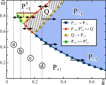
Figure 1: (Color online) Diagram of the precessional modes for $\sigma\rho=+1$. The regions in the $\tilde{h}$-$\tilde{\omega}$ plane where different P modes exist at $\sigma\rho=+1$ are denoted as $\rm{P}_{+1}$ (white) and $\rm{P}_{+1}^{{\dagger}}$ (light-green). The Q mode is realized in the white shaded region. In the region denoted as $\rm{P}_{-1}$ (blue) the stable precessional modes with $\sigma\rho=+1$ do not exist. Here, only the P mode with $\sigma\rho=-1$ is realized. The vertical dotted lines (a), (b), (c) and (d) correspond to $\tilde{h}=0.05,\;0.1,\;0.18$ and $0.25$, respectively.

Moreover, using Eq. (21) and the stability criterion for the P mode,DLHT we independently confirmed the correctness of this diagram by calculating the lines that separate the regions with $\sigma\rho=+1$.

Since the rotating field is switched on during the time interval of duration $\tilde{t}_{0}=(n-1)10^{3}$, the above procedure is time consuming. However, in view of the importance of the diagram of the precessional modes for the problem of lifetimes, its use for the precise determination of this diagram is quite acceptable. At the same time, the application of this method to the study of the steady-state properties of a given mode, whose character is already known from the diagram, is clearly redundant. Therefore, to reduce the computational time, next we use a modified numerical procedure with $\tilde{t}_{\rm{m}}=\Delta\tilde{t}$ and $\Delta\tilde{h}=\tilde{h}\Delta\tilde{t}/50$ leading to $\tilde{t}_{0}=\Delta\tilde{t}\,\tilde{h}/\Delta\tilde{h}=50$.

Figure 2 shows the frequency dependence of the precession angle $\Theta_{+1}$ for different precessional modes.

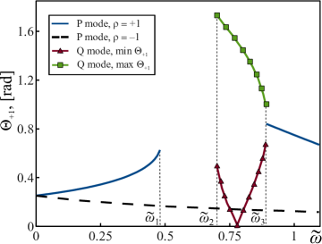
Figure 2: (Color online) Frequency dependence of the precession angle $\Theta_{+1}$ for different modes that exist at $\tilde{h}=0.25$. The frequencies $\tilde{\omega}_{1}=0.49$, $\tilde{\omega}_{2}=0.70$ and $\tilde{\omega}_{3}=0.89$ are the coordinates of the points in which the vertical dotted line (d), see Fig. 1, crosses the boundaries of the diagram ($\tilde{\omega}_{1}$, $\tilde{\omega}_{2}$, and $\tilde{\omega}_{3}$ depend on $\tilde{h}$). The green line (with squares) and brown line (with triangles) show the frequency dependence of $\max{\Theta_{+1}(\tilde{t})}$ and $\min{\Theta_{+1}(\tilde{t})}$, respectively, in the case of Q mode.

The dashed (black) and solid (blue) lines correspond to the P modes with $\sigma\rho=-1$ and $\sigma\rho=+1$, respectively. In accordance with Fig. 1, the Q mode occurs at $\tilde{\omega}_{2}<\tilde{\omega}<\tilde{\omega}_{3}$ (we recall that this mode can exist only if $\sigma\rho=+1$). For this mode, the time dependence of the precession angle $\Theta_{+1}(\tilde{t})$ and the time dependence of the difference of phases $\Psi_{+1}(\tilde{t})=-\nu\tilde{t}+\Phi_{+1}(\tilde{t})$ are illustrated in Figs. 3 and 4.

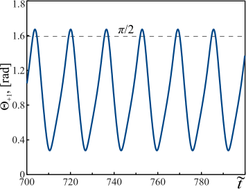
Figure 3: (Color online) Time dependence of the precession angle $\Theta_{+1}(\tilde{t})$ in the case of Q mode. The parameters of the rotating field are as follows: $\rho=+1$, $\tilde{\omega}=0.725$, and $\tilde{h}=0.25$.

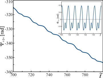
Figure 4: (Color online) Time dependence of the difference of phases $\Psi_{+1}(\tilde{t})=-\nu\tilde{t}+\Phi_{+1}(\tilde{t})$ in the case of Q mode. Insert: time dependence of the function $\Phi_{+1}(\tilde{t})$. The parameters of the rotating field are the same as in Fig. 3 and $\nu=0.38$.

We note that for a given set of parameters $\max{\Theta_{+1}(\tilde{t})}>\pi/2$, i.e., the precession angle $\Theta_{\sigma}(\tilde{t})$ in the case of Q mode can cross the anisotropy barrier. Moreover, since $\sin\Theta_{\sigma}(\tilde{t})$ and $\sin\Psi_{\sigma}(\tilde{t})$ have the same period $\tilde{T}_{Q}$, the parameter $\nu$ and the period $\tilde{T}_{Q}$ (its frequency dependence illustrates Figs. 5) are connected by the condition $\nu=2k\pi/\tilde{T}_{Q}$, where $k$ is a nonnegative integer

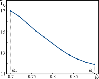
Figure 5: (Color online) Frequency dependence of the period $\tilde{T}_{Q}$ of the precession angle $\Theta_{+1}(\tilde{t})$ in the case of Q mode. The rotating field parameters are taken as $\rho=+1$ and $\tilde{h}=0.25$.

that depends on $\tilde{h}$ and $\tilde{\omega}$. In particular, if $\tilde{h}=0.25$ then $k=1$ at $\tilde{\omega}_{2}<\tilde{\omega}<\tilde{\omega}_{2}^{\prime}$, where $\tilde{\omega}_{2}^{\prime}=0.78$ is the solution of the equation $\min{\Theta_{+1}(\tilde{t})}|_{\tilde{\omega}=\tilde{\omega}_{2}^{\prime}}=0$ (see Fig. 2), and $k=0$ at $\tilde{\omega}_{2}^{\prime}<\tilde{\omega}<\tilde{\omega}_{3}$. It should also be stressed that in the last case the function $\Phi_{+1}(\tilde{t})$ shows a cosine-like behavior, in contrast to that shown in Fig. 4.

IV.2 Simulated lifetimes and their properties

As it was mentioned earlier, the thermal fluctuations can cause the transitions between different precessional modes induced by a given rotating field. According to the diagram in Fig. 1, these modes, one in the up state of the magnetic moment and the other in the down state, exist only if the amplitude and frequency of the rotating field belong to the region $P_{+1}$, $P_{+1}^{{\dagger}}$ or Q. In this case, the lifetime of a given mode can be calculated from the numerical solution of the stochastic equations (7). Our testing calculations showed that the solution of these equations by the Euler method gives practically the same lifetime obtained by the fourth order Runge-Kutta method. But in the first case the calculation time is almost four times less. Therefore, because the procedure of determining the frequency dependence of the lifetime is extremely time-consuming, we used the Euler method. The time step $\Delta\tilde{t}$ is chosen to be $10^{-3}$ and the initial conditions are given by $\theta_{\sigma}(0)=\pi(1-\sigma)/2+\sigma 10^{-2}$ and $\psi_{\sigma}(0)=0$. To prevent the appearance of singularities in Eq. (7) at $\theta_{\sigma}=\pi(1-\sigma)/2$, we assume that the point $\theta_{\sigma}=\pi(1-\sigma)/2+\sigma 10^{-3}$ acts on the process $\theta_{\sigma}(\tilde{t})$ as a reflecting screen. Since our interest here is the lifetimes of the precessional modes reaching the steady state, the thermal fluctuations are switched on at $\tilde{t}=\tilde{t}_{\rm{st}}$ (see Sec. II.2) with $\tilde{t}_{\rm{st}}=\tilde{t}_{0}+\tilde{t}_{\rm{rel}}$ (see Fig. 6). In the case of P modes we chose $\tilde{t}_{\rm{st}}=10^{2}$, while for the Q mode $\tilde{t}_{\rm{st}}\in[10^{2},10^{2}+\tilde{T}_{Q}]$. In the latter case, the thermal fluctuations can be switched on at a certain instant of time, e.g., when the precession angle $\Theta_{\sigma}(\tilde{t})$ reaches maximum or minimum. Finally, in all our numerical simulations the parameter $a=mH_{a}/2k_{B}T$ is chosen to be ten.

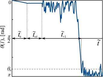
Figure 6: (Color online) Schematic time dependence of the polar angle $\theta(\tilde{t})$ in the regions $\rm{P}_{+1}$ and $\rm{P}_{+1}^{{\dagger}}$ shown in Fig. 1. The change of the magnetic moment state $\sigma$ from $+1$ to $-1$ occurs at $\tilde{t}=\tilde{t}_{0}+\tilde{t}_{\rm{rel}}+\tilde{t}_{+1}$, when $\theta(\tilde{t})$ reaches the angle $\theta_{0}=0.8\pi$ (the horizontal dashed line) for the first time. For a given trajectory $\theta(\tilde{t})$, the lifetime of the P mode in the state $\sigma=+1$ is equal to $\tilde{t}_{+1}$. Running $N\gg 1$ trajectories, the mean lifetime can be evaluated as $\mathcal{T}_{+1}=(1/N)\sum_{i=1}^{N}\tilde{t}_{+1}^{(i)}$.

In Fig. 7, we show the frequency dependencies of the lifetime $\mathcal{T}_{+1}$ for the rotating field amplitudes indicated in Fig. 1. Each point of these curves is determined by running $N=10^{4}$ trajectories of the polar angle $\theta(\tilde{t})$ (see the caption to Fig. 6).

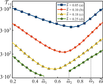
Figure 7: (Color online) Frequency dependencies of the lifetime of the precessional modes induced by the rotating field with $\rho=+1$ in the up state ($\sigma=+1$) of the magnetic moment.

If $\tilde{h}<0.19$ then the dependence of $\mathcal{T}_{+1}$ on $\tilde{\omega}$ is continuous and exhibits a resonant minimum at $\tilde{\omega}=\tilde{\omega}_{\rm{res}}$. The plot of the resonant frequency $\tilde{\omega}_{\rm{res}}$ versus the field amplitude $\tilde{h}$ is shown in Fig. 8. In contrast, if $\tilde{h}>0.19$ then $\mathcal{T}_{+1}$ is discontinuous: at $\tilde{\omega}\in(\tilde{\omega}_{1},\tilde{\omega}_{2})$ the function $\mathcal{T}_{+1}$ does not exist. This result is a consequence of the fact that in the region $\rm{P}_{-1}$ (see Fig. 1) there are no stable precessional modes with $\sigma\rho=+1$.

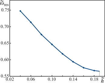
Figure 8: (Color online) Dependence of the resonant frequency of the lifetime $\mathcal{T}_{+1}$ on the rotating field amplitude.

One more important feature of the lifetime $\mathcal{T}_{+1}$ is that it is practically not sensitive to changing the character of the precessional modes. In particular, for $\tilde{h}=0.1$ the frequency dependence of $\mathcal{T}_{+1}$ (see the red line with circles in Fig. 7) is continuous at the point $\tilde{\omega}=0.74$ (i.e., point separating the regions $\rm{P}_{+1}$ and $\rm{P}_{+1}^{{\dagger}}$ at $\tilde{h}=0.1$), while the precession angle $\Theta_{+1}$ is discontinuous. This insensibility of the lifetime to changing the precessional modes with changing the field frequency $\tilde{\omega}$ is especially surprising when the Q mode appears. For example, even at $\tilde{h}=0.25$, when the precession angle can cross the anisotropy barrier (see Fig. 3), the character of the frequency dependence of $\mathcal{T}_{+1}$ (see the green line with stars in Fig. 7) is changed at $\tilde{\omega}=\tilde{\omega}_{3}$ so small that it is not visible on this scale. Moreover, the lifetime of the Q mode does almost not depend on $\tilde{t}_{\rm{st}}\in[10^{2},10^{2}+\tilde{T}_{Q}]$. This result is counterintuitive because different $\tilde{t}_{\rm{st}}$ may correspond to very different values of the precession angle $\Theta_{+1}(\tilde{t}_{\rm{st}})$. Therefore, in order to get more insight into the problem, we calculated the probability density function $D(\tilde{t}_{+1})$ of the lifetime of the Q mode for two special values of $\tilde{t}_{\rm{st}}$ which correspond to $\min\Theta_{+1}(\tilde{t})$ and $\max\Theta_{+1}(\tilde{t})$, respectively. As seen from Fig. 9, these density functions are somewhat different from each other only if $\tilde{t}_{+1}\lesssim\tilde{t}_{\rm{rel}}$. In this region the probability density $D(\tilde{t}_{+1})$ depends on $\tilde{t}_{\rm{st}}$ and exhibits local minima and maxima which come from a complex behavior of the Q mode. In contrast, at $\tilde{t}_{+1}\gg\tilde{t}_{\rm{rel}}$ the memory about the chosen value of $\tilde{t}_{\rm{st}}$ and periodicity of $\Theta_{+1}(\tilde{t})$ and $\Phi_{+1}(\tilde{t})$ is lost. As a consequence, in this region the difference between density functions vanishes and the local minima and maxima disappear. Such behavior of $D(\tilde{t}_{+1})$ on $\tilde{t}_{\rm{st}}$ confirms that the lifetime $\mathcal{T}_{+1}=\int_{0}^{\infty}d\tilde{t}_{+1}\,\tilde{t}_{+1}D(\tilde{t}_{+1})$ practically does not depend on $\tilde{t}_{\rm{st}}$.

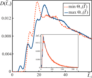
Figure 9: (Color online) Probability density functions of the lifetime of the Q mode for two values of $\tilde{t}_{\rm{st}}$. The blue solid and red dashed lines correspond to such $\tilde{t}_{\rm{st}}$ that $\Theta_{+1}(\tilde{t}_{\rm{st}})=\max\Theta_{+1}(\tilde{t})$ and $\Theta_{+1}(\tilde{t}_{\rm{st}})=\min\Theta_{+1}(\tilde{t})$, respectively. Insert: the same density functions in a larger time scale. The parameters of the rotating field are as follows: $\rho=+1$, $\tilde{\omega}=0.75$, and $\tilde{h}=0.25$.

Finally, the influence of the direction of field rotation on the frequency dependence of the lifetime of the precessional modes is illustrated in Fig. 10. In accordance with our analytical results, the rotating field with $\rho=+1$ and $\rho=-1$ influences the lifetime $\mathcal{T}_{+1}$ in a different way. Specifically, $\mathcal{T}_{+1}$ as a function of $\tilde{\omega}$ at $\rho=+1$ displays a deep minimum, while at $\rho=-1$ it shows a pronounced maximum.

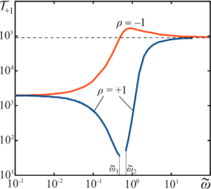
Figure 10: (Color online) Frequency dependencies of the lifetime of the precessional modes in the up state ($\sigma=+1$) of the magnetic moment. It is assumed that $\tilde{h}=0.25$ for both clockwise ($\rho=-1$) and counterclockwise ($\rho=+1$) rotation of the magnetic field.

This difference in the behavior of the lifetime results from that the rotating fields with different $\rho$ act on the magnetic moment in a given state $\sigma$ quite differently. From a physical point of view, the reason is that the magnetic moment has a definite direction of the natural precession. We note also that the numerical data $\mathcal{T}_{+1}|_{\tilde{\omega}\to\infty}=9.1\times 10^{4}$ and $\mathcal{T}_{+1}|_{\tilde{\omega}\to 0}=1.97\times 10^{3}$ are in a good agreement with the analytical results $8.2\times 10^{4}$ and $2.38\times 10^{3}$ obtained from the asymptotic formulas (55) and (64), respectively. Some difference between them can be caused by that the asymptotic formulas, which were obtained at $a\to\infty$, are applied to $a=10$.

V CONCLUSIONS

We have studied in detail the thermal stability of the precessional modes of the nanoparticle magnetic moment induced by the rotating magnetic field whose plane of rotation is perpendicular to the easy axis of the nanoparticle. If the direction of field rotation and the direction of the natural precession of the magnetic moment are opposite, i.e., if the condition $\sigma\rho=-1$ holds, then only periodic (P) stable mode is induced by this field. In contrast, if the above mentioned directions coincide, i.e., if $\sigma\rho=+1$, then the magnetic moment exhibits a much more complicated behavior. The numerical solution of the deterministic Landau-Lifshitz equation in the long-time limit has shown that, depending on the rotating field amplitude and frequency, in this case the magnetic moment can be in one of two P modes, in the quasi-periodic (Q) mode, or even be unstable. These results obtained in the absence of thermal fluctuations have been collected in the diagram shown in Fig. 1.

If the amplitude and frequency of the rotating field are chosen so that a stable precessional mode exists in both up ($\sigma=+1$) and down ($\sigma=-1$) states of the magnetic moment, then the thermal fluctuations can cause transitions between these modes. One of the most important parameters characterizing these transitions is the lifetime of a given mode. Since it can be naturally associated with the mean first-passage time for the magnetic moment, we have used the Fokker-Planck formalism to define this quantity and calculate its properties. In particular, we have determined the boundary conditions and transformation properties of the lifetime and have developed an analytical method for finding its frequency dependence in the case of high anisotropy barrier and small amplitudes of the rotating field. Using this method, it has been shown that the rotating field (a) slightly decreases (if $\sigma\rho=+1$) or increases (if $\sigma\rho=-1$) the lifetime of the P mode at large frequencies and (b) strongly decreases it (if $\sigma\rho=+1$) in the vicinity of the Larmor frequency. We have also established that at zero frequency the lifetime is always less than in the limit of large frequencies.

These analytical findings for the lifetime of the P mode have been confirmed by our numerical simulations of the stochastic Landau-Lifshitz equation. Moreover, the numerical simulations of this equation for not too small amplitudes of the rotating field permitted us to solve the problem of the lifetime of the Q mode. Since in this case the precession angle is a periodic function of time which can cross the anisotropy barrier, the solution of this problem is of particular interest. It has turned out that, although the precessional angle depends on time, the lifetime of the Q mode practically does not depend on this time, i.e., on the precession angle. We have also verified this result by calculating the lifetime from the first-passage time distributions that correspond to different values of the precession angle.

References

- (1) A. Moser, K. Takano, D. T. Margulies, M. Albrecht, Y. Sonobe, Y. Ikeda, S. Sun, and E. E. Fullerton, J. Phys. D: Appl. Phys. 35, R157 (2002).
- (2) C. A. Ross, Annu. Rev. Mater. Res. 31, 203 (2001).
- (3) I. Žutić, J. Fabian, and S. Das Sarma, Rev. Mod. Phys. 76, 323 (2004).
- (4) S. A. Wolf, D. D. Awschalom, R. A. Buhrman, J. M. Daughton, S. von Molnár, M. L. Roukes, A. Y. Chtchelkanova, and D. M. Treger, Sciense 294, 1488 (2001).
- (5) S. Laurent, D. Forge, M. Port, A. Roch, C. Robic, L. Vander Elst, and R. N. Muller, Chem. Rev. 108, 2064 (2008).
- (6) M. Ferrari, Nat. Rev. Cancer 5, 161 (2005).
- (7) Q. A. Pankhurst, J. Connolly, S. K. Jones, and J. Dobson, J. Phys. D: Appl. Phys. 36, R167 (2003).
- (8) H. J. Richter, J. Phys. D: Appl. Phys. 40, R149 (2007).
- (9) H. Risken, The Fokker-Planck Equation, 2nd ed. (Springer-Verlag, Berlin, 1989).
- (10) W. F. Brown, Jr., Phys. Rev. 130, 1677 (1963).
- (11) W. T. Coffey, Yu. P. Kalmykov, and J. T. Waldron, The Langevin Equation, 2nd ed. (World Scientific, Singapore, 2004).
- (12) P. Hänggi, P. Talkner, and M. Borkovec, Rev. Mod. Phys. 62, 251 (1990).
- (13) C. W. Gardiner, Handbook of Stochastic Methods, 2nd ed. (Springer-Verlag, Berlin, 1990).
- (14) S. Redner, A Guide to First-Passage Processes (Cambridge University Press, Cambridge, 2001).
- (15) S. I. Denisov and A. N. Yunda, Physica B 245, 282 (1998).
- (16) S. I. Denisov, T. V. Lyutyy, and K. N. Trohidou, Phys. Rev. B 67, 014411 (2003).
- (17) C. Thirion, W. Wernsdorfer, and D. Mailly, Nat. Mater. 2, 524 (2003).
- (18) Z. Z. Sun and X. R. Wang, Phys. Rev. B 73, 092416 (2006).
- (19) Z. Z. Sun and X. R. Wang, Phys. Rev. B 74, 132401 (2006).
- (20) J. Podbielski, D. Heitmann, and D. Grundler, Phys. Rev. Lett. 99, 207202 (2007).
- (21) G. Woltersdorf and C. H. Back, Phys. Rev. Lett. 99, 227207 (2007).
- (22) J. G. Zhu, X. Zhu, and Y. Tang, IEEE Trans. Magn. 44, 125 (2008).
- (23) G. Bertotti, C. Serpico, and I. D. Mayergoyz, Phys. Rev. Lett. 86, 724 (2001).
- (24) G. Bertotti, I. D. Mayergoyz, and C. Serpico, Physica B 343, 325 (2004).
- (25) S. I. Denisov, T. V. Lyutyy, P. Hänggi, and K. N. Trohidou, Phys. Rev. B 74, 104406 (2006).
- (26) G. Bertotti, I. D. Mayergoyz, C. Serpico, M. d’Aquino, and R. Bonin, J. Appl. Phys. 105, 07B712 (2009).
- (27) L. Chotorlishvili, P. Schwab, and J. Berakdar, J. Phys.: Condens. Matter 22, 036002 (2010).
- (28) G. Bertotti, I. Mayergoyz, and C. Serpico, Nonlinear Magnetization Dynamics in Nanosystems (Elsevier, Oxford, 2009).
- (29) S. I. Denisov, T. V. Lyutyy, C. Binns, P. Hänggi, J. Magn. Magn. Mater. 322, 1360 (2010).
- (30) T. V. Lyutyy, A. Yu. Polyakov, A. V. Rot-Serov, and C. Binns, J. Phys.: Condens. Matter 21, 396002 (2009).
- (31) S. I. Denisov, T. V. Lyutyy, P. Hänggi, Phys. Rev. Lett. 97, 227202 (2006).
- (32) S. I. Denisov, K. Sakmann, P. Talkner, and P. Hänggi, Europhys. Lett. 76, 1001 (2006).
- (33) S. I. Denisov, K. Sakmann, P. Talkner, and P. Hänggi, Phys. Rev. B 75, 184432 (2007).
- (34) R. Kubo and N. Hashitsume, Prog. Theor. Phys. Suppl. 46, 210 (1970).
- (35) See Eq. 2.1.9.3 in A. D. Polyanin and V. F. Zaitsev, Handbook of Exact Solutions for Ordinary Differential Equations (CRC, Boca Raton, 1995).
- (36) F. W. J. Olver, Introduction to Asymptotics and Special Functions (Academic, New York, 1974).
- (37) C. H. Back, R. Allenspach, W. Weber, S. S. P. Parkin, D. Weller, E. L. Garwin, and H. C. Siegmann, Science 285, 864 (1999).