Characterizing the Heavy Elements in Globular Cluster M22 and an Empirical $s$-process Abundance Distribution Derived from the Two Stellar Groups

Abstract

We present an empirical $s$-process abundance distribution derived with explicit knowledge of the $r$-process component in the low-metallicity globular cluster M22. We have obtained high-resolution, high signal-to-noise spectra for 6 red giants in M22 using the MIKE spectrograph on the Magellan-Clay Telescope at Las Campanas Observatory. In each star we derive abundances for 44 species of 40 elements, including 24 elements heavier than zinc ($Z=$ 30) produced by neutron-capture reactions. Previous studies determined that 3 of these stars (the “$r+s$ group”) have an enhancement of $s$-process material relative to the other 3 stars (the “$r$-only group”). We confirm that the $r+s$ group is moderately enriched in Pb relative to the $r$-only group. Both groups of stars were born with the same amount of $r$-process material, but $s$-process material was also present in the gas from which the $r+s$ group formed. The $s$-process abundances are inconsistent with predictions for AGB stars with $M\leq$ 3 $M_{\odot}$ and suggest an origin in more massive AGB stars capable of activating the ²²Ne($\alpha$,$n$)²⁵Mg reaction. We calculate the $s$-process “residual” by subtracting the $r$-process pattern in the $r$-only group from the abundances in the $r+s$ group. In contrast to previous $r$- and $s$-process decompositions, this approach makes no assumptions about the $r$- and $s$-process distributions in the solar system and provides a unique opportunity to explore $s$-process yields in a metal-poor environment.

1. Introduction

By the time the average global star formation rate peaked in galaxies destined to grow to the size of the Milky Way 1–3 Gyr after the Big Bang, vigorous heavy metal enrichment had already begun. Elements heavier than the Fe-group are traditionally understood to be produced mainly by two processes, the rapid and slow neutron-capture processes. The $r$-process (“$r$” for rapid) manufactures heavy nuclei by overwhelming existing nuclei with a rapid neutron burst on timescales $\sim$ 1 s, far shorter than the average $\beta$-decay timescales that could return unstable nuclei to stable ones. The $s$-process (“$s$” for slow) manufactures heavy nuclei by adding neutrons to existing nuclei on timescales slow relative to the average $\beta$-decay rates. Each of these two neutron ($n$) capture processes contributes about half of the heavy elements in the solar system (S.S.), which samples the chemistry of the interstellar medium (ISM) at one point in the Milky Way disc more than 9 Gyr after the big bang. The $r$-process requires an explosive, neutron-rich environment, suggesting an association with the core collapse supernovae (SNe) that claim the lives of massive stars ($M\gtrsim$ 8 $M_{\odot}$), while the $s$-process may be activated in less massive stars (1 $\lesssim M\lesssim$ 8 $M_{\odot}$) during their asymptotic giant branch (AGB) phase of evolution. Enrichment of the ISM by $r$-process material may begin a few tens of Myr after star formation commences, while $s$-process enrichment requires at least 50 Myr to several Gyr depending on the AGB mass ranges involved.

After an early description of the $s$-process by B²FH (1957), Clayton et al. (1961) and Seeger et al. (1965) developed the phenomenological (also known as the “classical”) approach that dominated $s$-process modeling for decades to follow. This method takes advantage of the fact that the product of the $n$-capture cross section and the $s$-process abundance of each isotope is slowly variable and can be approximated locally as a constant. These authors also recognized that a single neutron flux is insufficient to reproduce the $s$-only isotopes in the S.S. (See also Clayton & Rassbach 1967.) In order to explain the $s$-process distribution in the S.S., at least 3 components are required, known today as the “main,” “weak,” and “strong” components. The main component accounts for isotopes from 90 $\lesssim A\leq$ 207, the weak component accounts for the bulk of the production of isotopes with $A\lesssim$ 90, and the strong component accounts for more than half of ²⁰⁸Pb.

More and improved experimental data collected over subsequent decades revealed the shortcomings of this phenomenological approach (e.g., Käppeler, Beer, & Wisshak 1989). Predictions of $s$-process yields made by post-processing stellar evolution models with reaction networks (e.g., Arlandini et al. 1999) improved the fit, particularly near the closed neutron shells at $N=$ 50, 82, and 126. Eventually the full reaction networks were integrated into the stellar evolution codes (e.g., Straniero, Gallino, & Cristallo 2006; Cristallo et al. 2009). Nucleosynthesis via the $s$-process depends on a number of variables including mass, metallicity, and $s$-process efficiency. Uncertainties in the mass dredged up after each thermal instability (which brings $s$-process material to the surface) and the mass-loss rate further complicate predictions. Detailed models are constrained by spectroscopic observations of $s$-process material in intrinsic (i.e., self-enriched) stars or extrinsic (i.e., enriched by a binary companion or born with the $s$-process material) ones. These models have mainly focused on low- and intermediate-mass AGB stars (i.e., $\leq$ 3 $M_{\odot}$) and are quite successful at reproducing both the S.S. $s$-process isotopic distribution and the elemental distributions observed in a variety of stars (e.g., Smith & Lambert 1986; Lambert et al. 1995; Busso et al. 1999, 2001; Bisterzo et al. 2009, 2011).

The $s$-process efficiency is largely governed by the conditions that activate reactions to liberate neutrons, and two sources of neutrons have been identified in AGB stars. The first, the ¹³C($\alpha$,$n$)¹⁶O reaction, is activated at temperatures around 1$\times$10⁸ K. ¹³C is of primary origin, synthesized from proton captures on freshly produced ¹²C. The ¹³C pocket is thought to form in the top layers of the region between the H and He shell-burning regions when protons from the H envelope are mixed into this region during the third dredge up. The amount of ¹³C in the pocket can be thought of as one measure of the $s$-process efficiency. The other source, the ²²Ne($\alpha$,$n$)²⁵Mg reaction, is activated at somewhat higher temperatures near 3.5$\times$10⁸ K. ²²Ne is also primary. It is produced by the reaction sequence ¹⁴N($\alpha$,$\gamma$)¹⁸F($\beta^{+}\nu$)¹⁸O($\alpha$,$\gamma$)²²Ne, where ¹⁴N is also primary as the most abundant product of CNO burning. Neutron densities from the ¹³C and ²²Ne reactions may reach $\sim$ 10⁷ cm^-3 and $\gtrsim$ 10¹¹ cm^-3, respectively. See, e.g., reviews by Busso, Gallino, & Wasserburg (1999) and Straniero et al. (2006) for further details.

The heavy elements in the S.S. are the products of many and various stars, and the stellar evolution parameter space necessary to fully reproduce the S.S. $s$-process pattern is vast and gradually being explored. Only in the S.S. is the complete heavy element inventory known with great precision at the isotopic level (e.g., Lodders 2003). Isotopes that can only be formed by the $r$- or $s$-process are readily identified, but no element in the S.S. with 30 $<Z\leq$ 83 owes its presence entirely to the $r$- or $s$-process. Limited by the assumption that only two processes contribute, the $r$- and $s$-process content in S.S. material can be estimated by the formula $N_{\odot,r}=N_{\odot,{\rm tot}}-N_{\odot,s}$. That is, the $r$-process “residual” equals the total S.S. abundance minus the $s$-process contribution, which is obtained by either phenomenological or stellar models (e.g., Seeger et al. 1965, Cameron 1973, Käppeler et al. 1989). Nearly all abundance information in other stars is in the form of elemental abundances. In certain astrophysical environments only one process or the other contributes, enabling direct comparison with model predictions. The difficulty lies in identifying suitable stars whose heavy elements may be reliably interpreted as having originated in only one process or the other.

One such star, CS 22892–052, with a metallicity less than 1/1000 solar ([Fe/H] $=-3.1$), was discovered in the survey of Beers, Preston, & Shectman (1992). CS 22892–052 has a heavy element abundance pattern that very nearly matches the scaled $r$-process residuals in the S.S. (e.g., Sneden et al. 1994, Cowan et al. 1995). Several other metal-poor stars with this pattern have been found, and nearly all stars analyzed to date contain detectable quantities of elements heavier than the Fe-group. These elements are frequently attributed to $r$-process nucleosynthesis (e.g., Truran 1981, McWilliam 1998, Sneden, Cowan, & Gallino 2008, Roederer et al. 2010b). The consistent $r$-process abundance pattern observed in several stars heavily enriched by $r$-process material inspired the idea that $r$-process abundances everywhere (at least for $Z\geq$ 56) may be scaled versions of the same pattern; however, stars with less extreme levels of $r$-process enrichment clearly deviate from this pattern (e.g., Honda et al. 2007, Roederer et al. 2010b).

Some metal-poor stars contain $s$-process material mixed with the $r$-process contribution. Obtaining an empirical measure of the $s$-process content in stars other than the sun is difficult because a level of $r$-process enrichment must be assumed. The metal-poor globular cluster (GC) M22 provides an opportunity to probe $s$-process enrichment in a low-metallicity environment where the $r$-process content is explicitly known. Recent spectroscopic studies have demonstrated that star-to-star variations in heavy elements exist in M22 (Marino et al., 2009, 2011b). This metal-poor ([Fe/H] $=-$1.76 $\pm$ 0.10) GC hosts two groups of stars, each with different amounts of heavy elements (Y, Zr, Ba, La, Nd) that in the S.S. are overwhelmingly due to the $s$-process (e.g., Simmerer et al. 2004). Marino et al. showed that the abundances of these elements, together with the total C$+$N$+$O and overall Fe-group abundances, increase as a function of metallicity. In contrast, [Eu/Fe] has no metallicity dependence (only 3% of S.S. Eu was produced by the $s$-process), demonstrating that the heavy element variations are due to different amounts of $s$-process material. Thus, the chemistry of M22 suggests one stellar group formed from gas enriched by $r$-process nucleosynthesis and a second group formed from gas also enriched in $s$-process material. Multiple stellar groups in M22 are also revealed in a split in the sub-giant branch (SGB) revealed by Hubble Space Telescope photometry (Piotto, 2009; Marino et al., 2009).

Table 1Photometry, Atmospheric Parameters, Radial Velocities, Exposure Times, and S/N Estimates

Star	$V$	$(B-V)_{0}$	$T_{\rm eff}$	log g	$v_{\rm t}$	[Fe/H]	RV	$t_{\rm exp}$	S/N	S/N	S/N	S/N
			(K)		(km s-1)		(km s-1)	(s)	(3950Å)	(4550Å)	(5200Å)	(6750Å)
I-27	12.39	1.28	4455	1.45	1.60	$-$1.73	$-$127.8	2600	40/1	95/1	95/1	210/1
I-37	12.01	1.45	4370	1.05	1.50	$-$1.73	$-$157.7	3800	50/1	125/1	140/1	340/1
I-53	12.69	1.36	4500	1.35	1.55	$-$1.74	$-$145.4	3000	45/1	105/1	120/1	270/1
I-80	12.53	1.38	4460	1.15	1.55	$-$1.70	$-$149.8	3100	40/1	90/1	100/1	230/1
III-33	12.25	1.40	4430	1.05	1.70	$-$1.78	$-$145.8	1600	45/1	105/1	120/1	275/1
IV-59	11.93	1.45	4400	1.00	1.70	$-$1.77	$-$152.8	1600	45/1	110/1	125/1	300/1

The chemical pattern revealed in M22 makes this GC a suitable target to investigate $s$-process abundance distributions. Observations indicate that the $r$-process content of both stellar groups in M22 is the same. Observations also indicate that the more metal-rich group (hereafter referred to as the “$r+s$ group”) was formed from gas also enriched by $s$-process material. We can subtract the $r$-process abundance pattern (established empirically in the metal-poor group, hereafter referred to as the “$r$-only group”) from the abundance pattern in the $r+s$ group to derive an empirical $s$-process abundance distribution. One favorable aspect of this approach is that it does not rely on the decomposition of S.S. material into $r$- or $s$-process fractions to interpret abundances elsewhere in the Galaxy.

2. Observations

Six probable members of M22 were observed with the Magellan Inamori Kyocera Echelle (MIKE) spectrograph (Bernstein et al., 2003) on the 6.5 m Magellan-Clay Telescope at Las Campanas Observatory on 2011 March 17–18. These spectra were taken with the 0.7”$\times$5.0” slit yielding a resolving power of $R\sim$ 41,000 in the blue and $R\sim$ 35,000 in the red, split by a dichroic around 4950Å. This setup provides complete wavelength coverage from 3350–9150Å, though in practice we only make use of the region from 3690 to 7800Å where the lines of interest are located. Data reduction, extraction, and wavelength calibration were performed using the MIKE data reduction pipeline written by D. Kelson. (See also Kelson 2003). Continuum normalization and order stitching were performed within the IRAF environment.

The six observed stars are all cool giants on the M22 red giant branch (RGB). Table 1 lists the photometry from the Stetson database (priv. communication, corrected for differential reddening as in Marino et al. 2011b) atmospheric parameters (adopted from Marino et al.; see Section 3), Heliocentric radial velocities (RV), exposure times, and signal-to-noise (S/N) estimates for our targets. We estimate the S/N based on Poisson statistics for the number of photons collected in the continuum. We measure the RV with respect to the ThAr lamp by cross correlating the echelle order containing the Mg i b lines in each spectrum against a template using the fxcor task in IRAF. We create the template by measuring the wavelengths of unblended Fe i lines in this order in star IV-59, which has the highest S/N in a single exposure. We compute velocity corrections to the Heliocentric rest frame using the IRAF rvcorrect task. This method yields a total uncertainty of 0.8 km s^-1 per observation (see Roederer et al. 2010a). Our RVs are in good agreement ($\Delta=$ 0.7 $\pm$ 0.7 km s^-1) with those derived by Marino et al. (2009) for 4 stars in common.

3. Abundance Analysis

We perform a standard abundance analysis on the 6 stars observed with MIKE. We adopt the atmospheric parameters derived by Marino et al. (2011b) and use $\alpha$-enhanced ATLAS9 model atmospheres from Castelli & Kurucz (2004). We perform the analysis using the latest version of the spectral analysis code MOOG (Sneden, 1973), with updates to the calculation of the Rayleigh scattering contribution to the continuous opacity described in Sobeck et al. (2011). We measure equivalent widths (EWs) by fitting Voigt absorption line profiles to the continuum-normalized spectra, and we derive abundances of Na i, Mg i, Al i, Si i, K i, Ca i, Ti i and ii, Cr i and ii, Fe i and ii, Ni i, and Zn i from a standard EW analysis. Abundances of all other elements are derived by spectral synthesis, comparing synthetic spectra to the observations. This is necessary for species whose lines may be blended, have broad hyperfine structure (HFS), or have multiple isotopes whose electronic levels are shifted slightly. The linelist, atomic data and references, and derived abundances for each line are presented in Table 3, which is available in the online-only edition.

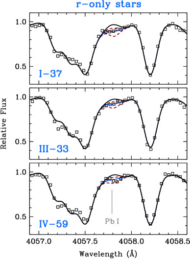
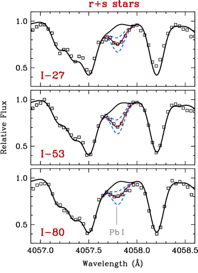
Figure 1.— Comparison of observed (open squares) and synthetic (lines) spectra around the Pb i 4057.8Å line. The left panels show the 3 $r$-only stars, and the right panels show the 3 $r+s$ stars. The solid colored line (left panels, blue; right panels, red) indicates the best-fit abundance, the dashed lines indicate variations in the best-fit abundance by 0.3 dex, and the solid black line indicates a synthesis with no Pb i present.

Table 2Line-by-line Abundances

Species	$\lambda$	E.P.	$\log(gf)$	Ref.	I-37	III-33	IV-59	I-27	I-53	I-80
	(Å)	(eV)
Na i	5682.63	2.10	$-$0.71	1	4.68	4.09	4.95	4.69	4.70	5.10
Na i	5688.20	2.10	$-$0.45	1	4.81	4.19	5.05	4.88	4.81	5.18
Na i	6154.23	2.10	$-$1.55	1	4.63	4.07	4.98	$\cdots$	4.63	5.04
Na i	6160.75	2.10	$-$1.25	1	4.77	4.13	4.89	4.68	4.67	5.13

References. — (1) Fuhr & Wiese (2009); (2) Chang & Tang (1990); (3) Lawler & Dakin (1989), using HFS from Kurucz & Bell (1995); (4) Blackwell et al. (1982a, b), increased by 0.056 dex according to Grevesse et al. (1989); (5) Pickering et al. (2001), with corrections given in Pickering et al. (2002); (6) Whaling et al. (1985), using HFS from Kurucz & Bell (1995); (7) Sobeck et al. (2007); (8) Nilsson et al. (2006); (9) Blackwell-Whitehead & Bergemann (2007), using HFS from Kurucz & Bell (1995); (10) Booth et al. (1984), using HFS from Kurucz & Bell (1995) (11) O’Brian et al. (1991); (12) Meléndez & Barbuy (2009); (13) Nitz et al. (1999), using HFS from Kurucz & Bell (1995); (14) Cardon et al. (1982), using HFS from Kurucz & Bell (1995); (15) Wickliffe & Lawler (1997a); (16) Bielski (1975), using HFS from Kurucz & Bell (1995); (17) Biémont & Godefroid (1980); (18) Migdalek & Baylis (1987); (19) Hannaford et al. (1982); (20) Biémont et al. (1981); (21) Ljung et al. (2006); (22) Whaling & Brault (1988); (23) Wickliffe et al. (1994); (24) Duquette & Lawler (1985); (25) Fuhr & Wiese (2009), using HFS from McWilliam (1998); (26) Lawler et al. (2001a), using HFS from Ivans et al. (2006); (27) Lawler et al. (2009); (28) Li et al. (2007), using HFS from Sneden et al. (2009); (29) Ivarsson et al. (2001), using HFS from Sneden et al. (2009); (30) Den Hartog et al. (2003); (31) Lawler et al. (2006); (32) Lawler et al. (2001b), using HFS from Ivans et al. (2006); (33) Den Hartog et al. (2006); (34) Lawler et al. (2001c), using HFS from Lawler et al. (2001d); (35) Wickliffe et al. (2000); (36) Lawler et al. (2004) for both $\log(gf)$ value and HFS; (37) Lawler et al. (2008); (38) Wickliffe & Lawler (1997b); (39) Sneden et al. (2009) for both $\log(gf)$ value and HFS; (40) Lawler et al. (2007); (41) Ivarsson et al. (2003); (42) Biémont et al. (2000); (43) Nilsson et al. (2002).

Note. — The full version of this table is available in the online edition of the journal. A limited version is given here to indicate the form and content of the data. Abundances are given as $\log\epsilon$ notation. A “:” indicates the derived abundance is less secure, and we estimate an uncertainty of 0.2 dex. See text for details.

In Figure 1 we show synthetic spectra fits to the region around the Pb i line at 4057Å. The solid lines represent the best-fit abundance, and the dashed lines represent variations in this fit by 0.3 dex. The 6 stars in our sample have very similar atmospheric parameters. In our syntheses we adjust the linelist to fit blending features in one star and leave these adjustments unchanged in the analysis of other stars. This preserves a differential quality in the abundance analysis, which is important in the case of abundances derived from very few or heavily blended lines.

Table 3Effect of Different Analysis Tools on Derived Abundances in I-37

$\lambda$ (Å)	$\log\epsilon$	$\log\epsilon$	$\log\epsilon$	$\log\epsilon$
La ii Lines
3988.51	$-$0.74	$-$0.66	$-$0.71	$-$0.61
3995.74	$-$0.70	$-$0.56	$-$0.69	$-$0.51
4086.71	$-$0.78	$-$0.70	$-$0.70	$-$0.56
4322.50	$-$0.70	$-$0.67	$-$0.68	$-$0.66
4662.50	$-$0.54	$-$0.50	$-$0.55	$-$0.46
4748.73	$-$0.65	$-$0.65	$-$0.62	$-$0.70
4804.04	$-$0.44	$-$0.43	$-$0.43	$-$0.53
4920.98	$-$0.34	$-$0.31	$-$0.28	$-$0.25
4986.82	$-$0.49	$-$0.48	$-$0.47	$-$0.41
5114.56	$-$0.48	$-$0.45	$-$0.43	$-$0.42
5290.84	$-$0.73	$-$0.69	$-$0.71	$-$0.64
5303.53	$-$0.45	$-$0.46	$-$0.44	$-$0.45
6262.29	$-$0.44	$-$0.45	$-$0.41	$-$0.41
6390.48	$-$0.39	$-$0.42	$-$0.38	$-$0.40
Mean:	$-$0.56	$-$0.53	$-$0.54	$-$0.50
$\sigma$:	0.15	0.12	0.15	0.12
$\sigma/\sqrt{N}$:	0.040	0.033	0.038	0.033
Ce ii Lines
4073.47	$-$0.35	$-$0.24	$-$0.32	$-$0.23
4083.22	$-$0.25	$-$0.17	$-$0.21	$-$0.14
4120.83	$-$0.20	$-$0.17	$-$0.17	$-$0.08
4127.36	$-$0.24	$-$0.20	$-$0.24	$-$0.15
4137.65	$-$0.26	$-$0.18	$-$0.20	$-$0.13
4222.60	$-$0.23	$-$0.19	$-$0.20	$-$0.16
4364.65	$-$0.21	$-$0.18	$-$0.19	$-$0.15
4418.78	$-$0.23	$-$0.15	$-$0.16	$-$0.08
4486.91	$-$0.26	$-$0.24	$-$0.24	$-$0.23
4560.96	$-$0.21	$-$0.19	$-$0.18	$-$0.17
4562.36	$-$0.17	$-$0.14	$-$0.14	$-$0.08
4572.28	$-$0.16	$-$0.11	$-$0.02	$+$0.00
4582.50	$-$0.05	$-$0.02	$-$0.05	$+$0.03
4628.16	$-$0.08	$-$0.07	$-$0.02	$+$0.04
5274.23	$-$0.20	$-$0.21	$-$0.22	$-$0.20
5330.56	$-$0.22	$-$0.24	$-$0.19	$-$0.22
Mean:	$-$0.21	$-$0.17	$-$0.17	$-$0.12
$\sigma$:	0.07	0.06	0.08	0.09
$\sigma/\sqrt{N}$:	0.017	0.015	0.020	0.021
$\log\epsilon$(La/Ce):	$-$0.35	$-$0.36	$-$0.36	$-$0.38
	$\pm$0.043	$\pm$0.036	$\pm$0.044	$\pm$0.039

The EWs measured by Marino et al. (2011b) from a high S/N VLT/UVES spectrum of I-27 are systematically higher by 4.9 $\pm$ 0.6 mÅ ($\sigma=$ 3.2 mÅ). the only case where the offset is larger than the standard deviation of the residuals (3.2–3.4 mÅ in all stars). In I-27, this translates to no significant difference in the derived [X/Fe] ratios (since both abundances are similarly affected), $\Delta$[X/Fe] $=$ 0.00 $\pm$ 0.01 ($\sigma=$ 0.03 dex), and the change in metallicity is $\Delta$[Fe/H] $=$ 0.06. EWs measured from the lower S/N APO/ARC Echelle spectrum of I-27 analyzed by Marino et al. are systematically lower by 5.2 $\pm$ 2.6 mÅ ($\sigma=$ 11 mÅ). Differences at this level may be expected when analyzing spectra of various resolution and S/N, collected over many nights using instruments on different telescopes in different hemispheres, so we do not pursue the matter further. We also compare our derived abundance ratios with those presented in Marino et al. After accounting for the different sets of $\log(gf)$ values, S.S. abundances (see Marino et al. 2009), and line-by-line mean offsets (see Appendix), the abundance offsets for most [Fe/H] and [X/Fe] ratios can be immediately accounted for. Offsets in other species (Ti i, Cu i, Zn i, La ii, and Nd ii) are unexplained by these factors but probably result from the S/N and small numbers of features available in the spectra of Marino et al. For the purposes of the present study, we will focus on the internal abundance differences derived from our MIKE spectra.

Table 3 shows the internal abundance precision possible with this method when large numbers ($N>$ 10) of lines are available across the visible spectral range. For this test we derive the abundances of La ii and Ce ii in star I-37 using two grids of model atmospheres (MARCS, Gustafsson et al. 2008; ATLAS9, Castelli & Kurucz 2004) and different treatments of Rayleigh scattering in MOOG. The elemental abundances and ratios are not dependent on the choice of model atmosphere grids or the treatment of Rayleigh scattering. For example, as shown in Table 3, in response to the different analysis tools the derived $\log\epsilon$(La/Ce) ratio changes by no more than 0.03 dex, which is smaller than the statistical uncertainties (0.036 to 0.044 dex). Furthermore, the stars in our study were chosen to have similar colors (1.36 $\leq(B-V)_{0}\leq$ 1.52), metallicities ($-$1.80 $\leq$ [Fe/H] $\leq-$1.70), and atmospheric parameters (4370 $\leq\mbox{$T_{\rm eff}$}\leq$ 4500 K and 1.00 $\leq\mbox{log~{}{\it g}}\leq$ 1.45; all based on the values presented in Marino et al. 2011b). Thus a relative abundance analysis is appropriate, and in all subsequent discussion, tables, and figures we cite internal (i.e., observational) uncertainties only.

Table 4Mean Abundances in the Three $r$-only Stars

		I-37						III-33						IV-59
Species	$Z$	$\langle\log\epsilon\rangle$	$\langle$[X/Fe]$\rangle$	$N$	$\sigma$	$\sigma_{\mu}$		$\langle\log\epsilon\rangle$	$\langle$[X/Fe]$\rangle$	$N$	$\sigma$	$\sigma_{\mu}$		$\langle\log\epsilon\rangle$	$\langle$[X/Fe]$\rangle$	$N$	$\sigma$	$\sigma_{\mu}$
Na i	11	4.72	0.20	4	0.08	0.041		4.12	$-$0.26	4	0.05	0.026		4.97	0.53	4	0.07	0.033
Mg i	12	6.25	0.37	3	0.21	0.121		6.17	0.43	3	0.17	0.101		6.16	0.36	3	0.20	0.115
Al i	13	4.89	0.16	4	0.09	0.047		4.50	$-$0.09	1	0.11	0.110		5.33	0.68	4	0.11	0.053
Si i	14	5.89	0.10	3	0.24	0.140		5.80	0.16	3	0.17	0.098		5.86	0.15	3	0.18	0.104
K i	19	4.12	0.81	1	0.11	0.110		3.93	0.76	1	0.11	0.110		4.06	0.83	1	0.11	0.110
Ca i	20	5.04	0.41	8	0.11	0.038		4.84	0.36	8	0.15	0.054		4.93	0.40	8	0.10	0.035
Sc ii	21	1.68	0.15	5	0.27	0.120		1.58	0.20	5	0.30	0.134		1.59	0.28	5	0.29	0.128
Ti i	22	3.28	0.05	9	0.07	0.022		3.11	0.03	9	0.07	0.022		3.25	0.11	9	0.08	0.027
Ti ii	22	3.79	0.47	9	0.12	0.039		3.58	0.40	9	0.10	0.035		3.64	0.53	9	0.09	0.031
V i	23	2.00	$-$0.21	5	0.10	0.045		1.97	$-$0.10	5	0.12	0.052		2.02	$-$0.11	5	0.09	0.040
Cr i	24	3.74	$-$0.18	6	0.12	0.049		3.62	$-$0.15	6	0.08	0.033		3.72	$-$0.12	6	0.07	0.029
Cr ii	24	4.14	0.13	1	0.11	0.110		4.00	0.13	1	0.11	0.110		3.95	0.15	1	0.11	0.110
Mn i	25	3.13	$-$0.59	4	0.12	0.061		3.12	$-$0.45	4	0.12	0.058		3.16	$-$0.47	4	0.12	0.061
Fe i	26	5.78	$-$1.72	69	0.13	0.016		5.63	$-$1.87	69	0.10	0.012		5.70	$-$1.80	69	0.12	0.015
Fe ii	26	5.87	$-$1.63	7	0.17	0.062		5.73	$-$1.77	7	0.08	0.031		5.66	$-$1.84	7	0.09	0.034
Co i	27	3.11	$-$0.16	4	0.09	0.043		3.01	$-$0.12	4	0.13	0.065		3.06	$-$0.13	4	0.18	0.089
Ni i	28	4.28	$-$0.23	10	0.10	0.033		4.20	$-$0.16	10	0.12	0.039		4.22	$-$0.19	10	0.11	0.034
Cu i	29	1.83	$-$0.65	2	0.08	0.057		1.64	$-$0.69	2	0.08	0.057		1.74	$-$0.65	2	0.08	0.057
Zn i	30	2.89	0.04	2	0.08	0.055		2.75	0.05	2	0.08	0.057		2.80	0.04	2	0.08	0.057
Rb i	37	$<$1.00	$<$0.20	1	$\cdots$	$\cdots$		$<$1.10	$<$0.44	1	$\cdots$	$\cdots$		$<$1.10	$<$0.38	1	$\cdots$	$\cdots$
Sr i	38	0.60	$-$0.55	1	0.11	0.110		0.51	$-$0.50	1	0.11	0.110		0.54	$-$0.53	1	0.11	0.110
Y ii	39	0.34	$-$0.25	7	0.04	0.016		0.18	$-$0.26	7	0.07	0.026		0.18	$-$0.19	7	0.08	0.030
Zr i	40	0.69	$-$0.18	2	0.08	0.057		0.78	0.06	2	0.08	0.057		0.63	$-$0.15	2	0.12	0.085
Zr ii	40	1.06	0.11	3	0.09	0.054		1.04	0.23	3	0.09	0.050		1.05	0.31	3	0.09	0.050
Mo i	42	0.33	0.16	2	0.14	0.099		0.00	$-$0.02	1	0.20	0.200		0.12	0.04	3	0.28	0.164
Ru i	44	0.09	0.06	3	0.14	0.082		0.07	0.18	3	0.13	0.075		0.18	0.23	1	0.20	0.200
Rh i	45	$-$0.84	$-$0.18	1	0.11	0.110		$\cdots$	$\cdots$	0	$\cdots$	$\cdots$		$-$1.16	$-$0.42	1	0.11	0.110
Ba ii	56	0.76	0.20	2	0.08	0.057		0.53	0.12	2	0.15	0.105		0.53	0.19	2	0.18	0.130
La ii	57	$-$0.54	$-$0.01	14	0.14	0.038		$-$0.59	0.09	14	0.08	0.022		$-$0.61	0.13	14	0.11	0.029
Ce ii	58	$-$0.17	$-$0.13	16	0.08	0.020		$-$0.26	$-$0.06	16	0.05	0.013		$-$0.29	$-$0.03	16	0.07	0.018
Pr ii	59	$-$0.87	0.04	4	0.05	0.025		$-$0.87	0.18	4	0.08	0.040		$-$0.93	0.19	4	0.05	0.025
Nd ii	60	$-$0.13	0.07	24	0.08	0.017		$-$0.18	0.18	24	0.07	0.014		$-$0.22	0.20	24	0.08	0.016
Sm ii	62	$-$0.48	0.19	9	0.07	0.022		$-$0.51	0.30	9	0.07	0.022		$-$0.55	0.33	9	0.07	0.023
Eu ii	63	$-$0.85	0.26	3	0.20	0.113		$-$0.88	0.37	3	0.15	0.085		$-$0.92	0.40	3	0.17	0.096
Gd ii	64	$-$0.30	0.25	3	0.14	0.081		$-$0.35	0.35	3	0.16	0.092		$-$0.41	0.36	3	0.11	0.061
Tb ii	65	$-$1.48	$-$0.15	1	0.11	0.110		$-$1.35	0.12	1	0.11	0.110		$-$1.67	$-$0.13	1	0.11	0.110
Dy ii	66	$-$0.20	0.33	4	0.13	0.063		$-$0.19	0.48	4	0.09	0.046		$-$0.37	0.37	4	0.29	0.144
Ho ii	67	$-$1.10	0.05	1	0.20	0.200		$-$1.15	0.14	1	0.20	0.200		$-$1.20	0.16	1	0.20	0.200
Er ii	68	$-$0.30	0.41	2	0.08	0.057		$-$0.48	0.37	2	0.10	0.070		$-$0.55	0.37	2	0.07	0.050
Tm ii	69	$-$1.43	0.10	2	0.18	0.125		$-$1.53	0.15	2	0.25	0.175		$-$1.65	0.09	2	0.07	0.050
Yb ii	70	$-$1.05	$-$0.34	1	0.20	0.200		$-$0.75	0.10	1	0.20	0.200		$-$1.00	$-$0.08	1	0.20	0.200
Hf ii	72	$-$1.00	$-$0.22	1	0.11	0.110		$-$0.93	$-$0.01	1	0.11	0.110		$-$1.09	$-$0.10	1	0.11	0.110
Ir i	77	0.00	0.34	1	0.11	0.110		$-$0.05	0.43	1	0.11	0.110		0.15	0.57	1	0.11	0.110
Pb i	82	0.05	$-$0.27	1	0.11	0.110		$-$0.01	$-$0.19	1	0.11	0.110		$-$0.08	$-$0.32	1	0.11	0.110
Th ii	90	$-$1.55	0.02	1	0.11	0.110		$-$1.42	0.29	1	0.11	0.110		$-$1.46	0.32	1	0.11	0.110

Note. — Quoted uncertainties represent internal uncertainties only. $\langle$[Fe/H]$\rangle$ is listed in the $\langle$[X/Fe]$\rangle$ column for Fe i and Fe ii.

Absolute uncertainties that account for errors in the derived atmospheric parameters are discussed in Marino et al. (2011b) and presented in Table 4 of that work. In the present study, if only 1 line of a particular species has been measured we adopt an uncertainty of 0.11 dex. This estimate is based on the mean standard deviation of individual lines for well-measured $n$-capture species (i.e., $N\geq$ 3). Some lines in Table 3 are marked with “:” to indicate that the derived abundance is less certain due to significant blending features, difficult continuum placement, etc. These lines have an adopted internal uncertainty of 0.2 dex.

Table 5Mean Abundances in the Three $r+s$ Stars

		I-27						I-53						I-80
Species	$Z$	$\langle\log\epsilon\rangle$	$\langle$[X/Fe]$\rangle$	$N$	$\sigma$	$\sigma_{\mu}$		$\langle\log\epsilon\rangle$	$\langle$[X/Fe]$\rangle$	$N$	$\sigma$	$\sigma_{\mu}$		$\langle\log\epsilon\rangle$	$\langle$[X/Fe]$\rangle$	$N$	$\sigma$	$\sigma_{\mu}$
Na i	11	4.75	0.39	3	0.16	0.092		4.70	0.27	4	0.08	0.039		5.11	0.62	4	0.06	0.029
Mg i	12	6.13	0.41	3	0.26	0.150		6.28	0.49	3	0.15	0.085		6.25	0.40	3	0.18	0.105
Al i	13	5.02	0.45	4	0.23	0.115		5.09	0.45	4	0.13	0.063		5.57	0.87	4	0.10	0.048
Si i	14	6.02	0.39	3	0.09	0.053		5.88	0.18	3	0.21	0.123		5.94	0.18	3	0.19	0.109
K i	19	4.14	0.99	1	0.11	0.110		4.09	0.87	1	0.11	0.110		4.12	0.84	1	0.11	0.110
Ca i	20	5.00	0.54	8	0.10	0.035		4.99	0.46	8	0.08	0.028		5.04	0.45	8	0.11	0.038
Sc ii	21	1.73	0.38	5	0.29	0.132		1.60	0.24	5	0.28	0.124		1.66	0.26	5	0.33	0.147
Ti i	22	3.05	$-$0.02	9	0.20	0.066		3.26	0.12	9	0.14	0.048		3.26	0.06	9	0.12	0.040
Ti ii	22	3.53	0.39	9	0.14	0.048		3.65	0.49	9	0.14	0.046		3.66	0.46	9	0.13	0.042
V i	23	2.06	0.02	5	0.15	0.066		1.98	$-$0.14	5	0.11	0.051		2.02	$-$0.16	5	0.16	0.072
Cr i	24	3.54	$-$0.22	6	0.17	0.067		3.67	$-$0.16	6	0.06	0.026		3.71	$-$0.18	6	0.07	0.030
Cr ii	24	3.99	0.15	1	0.11	0.110		4.05	0.20	1	0.11	0.110		4.26	0.37	1	0.11	0.110
Mn i	25	3.10	$-$0.45	4	0.16	0.080		3.08	$-$0.54	4	0.10	0.048		3.12	$-$0.56	4	0.13	0.063
Fe i	26	5.62	$-$1.88	69	0.17	0.020		5.68	$-$1.82	69	0.12	0.015		5.75	$-$1.75	69	0.13	0.016
Fe ii	26	5.70	$-$1.80	7	0.12	0.046		5.71	$-$1.79	7	0.13	0.048		5.75	$-$1.75	7	0.14	0.054
Co i	27	3.17	0.06	4	0.08	0.039		3.06	$-$0.12	4	0.13	0.064		3.15	$-$0.09	4	0.09	0.045
Ni i	28	4.24	$-$0.10	10	0.10	0.032		4.23	$-$0.17	10	0.08	0.027		4.31	$-$0.16	10	0.08	0.025
Cu i	29	1.95	$-$0.36	2	0.08	0.057		1.87	$-$0.51	2	0.08	0.057		1.84	$-$0.60	2	0.08	0.057
Zn i	30	2.89	0.21	2	0.08	0.057		3.03	0.28	2	0.11	0.080		3.08	0.27	2	0.10	0.070
Rb i	37	$<$1.30	$<$0.66	1	$\cdots$	$\cdots$		$<$1.20	$<$0.49	1	$\cdots$	$\cdots$		$<$1.35	$<$0.58	1	$\cdots$	$\cdots$
Sr i	38	1.08	0.09	1	0.11	0.110		1.08	0.02	1	0.11	0.110		0.97	$-$0.15	1	0.11	0.110
Y ii	39	0.77	0.36	7	0.08	0.031		0.69	0.27	7	0.05	0.017		0.72	0.26	7	0.09	0.035
Zr i	40	1.07	0.37	2	0.08	0.057		1.18	0.40	2	0.11	0.075		1.10	0.27	2	0.08	0.057
Zr ii	40	1.47	0.69	3	0.28	0.160		1.31	0.52	3	0.07	0.041		1.43	0.60	3	0.12	0.068
Mo i	42	0.32	0.32	3	0.45	0.259		0.37	0.30	3	0.55	0.388		0.18	0.05	2	0.23	0.130
Ru i	44	0.15	0.28	2	0.08	0.057		0.00	0.06	1	0.14	0.100		0.50	0.50	1	0.14	0.100
Rh i	45	$-$0.45	0.37	1	0.11	0.110		$-$0.55	0.20	1	0.20	0.200		$-$0.80	$-$0.11	1	0.11	0.110
Ba ii	56	1.20	0.82	2	0.08	0.057		1.13	0.74	2	0.08	0.057		1.09	0.66	2	0.08	0.057
La ii	57	$-$0.11	0.59	14	0.14	0.038		$-$0.13	0.56	14	0.07	0.020		$-$0.21	0.44	14	0.08	0.021
Ce ii	58	0.25	0.48	16	0.13	0.032		0.43	0.64	16	0.12	0.029		0.21	0.38	16	0.11	0.028
Pr ii	59	$-$0.60	0.49	4	0.06	0.029		$-$0.61	0.47	4	0.06	0.030		$-$0.72	0.31	4	0.06	0.030
Nd ii	60	0.22	0.61	24	0.10	0.020		0.19	0.56	24	0.09	0.019		0.06	0.39	24	0.09	0.019
Sm ii	62	$-$0.38	0.46	9	0.12	0.039		$-$0.33	0.50	9	0.09	0.029		$-$0.38	0.41	9	0.09	0.029
Eu ii	63	$-$1.05	0.23	3	0.26	0.149		$-$0.91	0.36	3	0.13	0.073		$-$0.91	0.32	3	0.11	0.065
Gd ii	64	$-$0.25	0.48	3	0.11	0.065		$-$0.15	0.57	3	0.12	0.070		$-$0.32	0.37	2	0.22	0.155
Tb ii	65	$\cdots$	$\cdots$	0	$\cdots$	$\cdots$		$-$1.28	0.21	1	0.11	0.110		$-$1.30	0.15	1	0.11	0.110
Dy ii	66	$-$0.25	0.46	3	0.14	0.079		$-$0.08	0.61	4	0.13	0.067		$-$0.16	0.49	3	0.06	0.035
Ho ii	67	$-$1.15	0.17	1	0.20	0.200		$-$1.18	0.13	1	0.20	0.200		$-$1.20	0.07	1	0.20	0.200
Er ii	68	$-$0.41	0.47	2	0.16	0.110		$-$0.43	0.45	2	0.19	0.135		$-$0.25	0.59	2	0.13	0.095
Tm ii	69	$\cdots$	$\cdots$	0	$\cdots$	$\cdots$		$-$1.50	0.19	1	0.20	0.200		$\cdots$	$\cdots$	0	$\cdots$	$\cdots$
Yb ii	70	$-$0.76	0.12	1	0.11	0.110		$-$0.56	0.31	1	0.11	0.110		$-$0.52	0.31	1	0.11	0.110
Hf ii	72	$-$0.56	0.39	1	0.11	0.110		$-$0.55	0.39	1	0.11	0.110		$-$0.60	0.30	1	0.11	0.110
Ir i	77	$\cdots$	$\cdots$	0	$\cdots$	$\cdots$		$\cdots$	$\cdots$	0	$\cdots$	$\cdots$		$\cdots$	$\cdots$	0	$\cdots$	$\cdots$
Pb i	82	0.77	0.61	1	0.11	0.110		0.97	0.74	1	0.11	0.110		0.63	0.34	1	0.11	0.110
Th ii	90	$\cdots$	$\cdots$	0	$\cdots$	$\cdots$		$\cdots$	$\cdots$	0	$\cdots$	$\cdots$		$\cdots$	$\cdots$	0	$\cdots$	$\cdots$

Note. — Quoted uncertainties represent internal uncertainties only. $\langle$[Fe/H]$\rangle$ is listed in the $\langle$[X/Fe]$\rangle$ column for Fe i and Fe ii.

One difficulty that is not minimized by our approach is that of comparing abundance ratios derived from species of different ionization states. Ratios of, e.g., [Ca/Fe] or [Eu/Fe] are computed by comparing Ca i to Fe i or Eu ii to Fe ii since both species of Fe are detected. Other ratios, such as [Pb/La] or [Pb/Eu], which compare Pb i to La ii or Eu ii, may be systematically uncertain. Note that for illustration purposes in the figures only we normalize the abundances of first-peak $n$-capture elements observed in their neutral state (Sr i, Mo i, Ru i, and Rh i) to the singly-ionized abundances by the difference in Zr ii and Zr i in each star (typically 0.2–0.4 dex).

4. Heavy Element Abundances in M22

In this section we analyze the abundance patterns in detail. The abundance results for each star in the $r$-only and $r+s$ groups are given in Tables 4 and 5, respectively. Table 6 lists the mean abundances for each element in the $r$-only and $r+s$ groups. We derive only upper limits from the Rb i line at 7800Å. Due to blending by CN and CH, we are unable to derive abundances of Ir i or Th ii in any star in the $r+s$ group.

4.1. The Light and Fe-group Abundance Patterns in M22

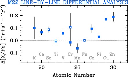
Figure 2.— Differences in the mean abundances between the 3 $r$-only stars and the 3 $r+s$ stars as a function of atomic number for K through Zn. Solid squares indicate neutral species, and open squares indicate singly-ionized species. The dotted line indicates zero difference.

We derive abundances of Na i, Mg i, Al i, and Si i in each star of the sample. After accounting for differences in the $\log(gf)$ values between this study and Marino et al. (2011b), these abundances are in agreement within the uncertainties. Marino et al. have discussed these abundances at length, so we shall not consider them further.

Marino et al. (2011b) detected an enhancement by 0.10 dex in the [Ca/Fe] ratio in the $r+s$ group of stars in M22, which we recover in our data. Other neighboring elements not included in that study also exhibit very slight differences in our data. To quantify these differences, we apply a line-by-line differential analysis, which is largely insensitive to uncertainties in the $\log(gf)$ values and star-to-star systematic effects in the abundance analysis. The differential results are listed in Table 7 and illustrated in Figure 2. When considering the standard error ($\sigma_{\mu}\equiv\sigma/\sqrt{N}$) of the mean line-by-line differential abundances (column 5), [K/Fe], [Ca/Fe], [Sc/Fe], and [V/Fe] show slight but significant (0.06–0.10 dex) enhancements in the $r+s$ group, [Ti/Fe] and [Cr/Fe] are indistinguishable in the two groups, and [Mn/Fe] shows a slight (0.06 dex) deficiency in the $r+s$ group.

Marino et al. (2011b) saw an increase by 0.06–0.15 dex in the [Cu/Fe] and [Zn/Fe] ratios of the $r+s$ group, which we also detect. Furthermore, we find a similar—though smaller—enhancement in [Co/Fe] and [Ni/Fe]. The results from a line-by-line differential analysis of these elements are also listed in Table 7 and shown in Figure 2.

A slight abundance enhancement in the Fe-group elements heavier than Fe may not be surprising, since $s$-process nucleosynthesis produces heavy nuclei from successive neutron capture on Fe-group seeds. Variations in the lighter Fe-group elements are more surprising. We return to this issue in Section 6.

4.2. The Neutron-Capture Abundance Patterns in M22

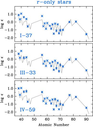
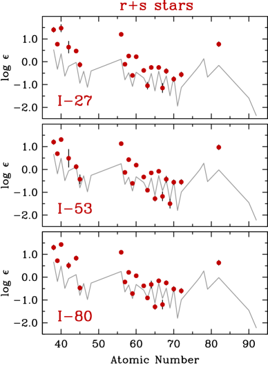
Figure 3.— Logarithmic abundances for $Z\geq$ 38 elements in the 3 $r$-only stars (blue crosses, left panels) and the 3 $r+s$ stars (red circles, right panels) as a function of atomic number. The gray line illustrates the abundances in the $r$-process standard star BD$+$17 3248 (Cowan et al., 2002, 2005; Sneden et al., 2009; Roederer et al., 2010c). Pb has not been detected in BD$+$17 3248, so we instead show the predicted Pb/Eu ratio based on the average Pb/Eu observed in Figure 3 of Roederer et al. (2010b). The BD$+$17 3248 abundance pattern has been normalized to the Eu abundance in each star.

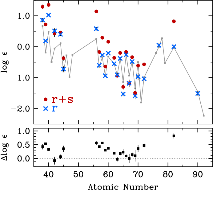
Figure 4.— Top panel: The mean logarithmic abundances for the 3 $r$-only stars (blue crosses) and the 3 $r+s$ stars (red circles) as a function of atomic number. The gray line and small gray squares illustrate the abundances in the $r$-process standard star BD$+$17 3248 (Cowan et al., 2002, 2005; Sneden et al., 2009; Roederer et al., 2010c). Pb has not been detected in BD$+$17 3248, so we instead show the predicted Pb/Eu ratio based on the average Pb/Eu observed in Figure 3 of Roederer et al. (2010b). The BD$+$17 3248 abundance pattern has been normalized to the Eu abundance. Bottom panel: The differences in these mean abundances. The dotted line indicates zero difference.

Figure 3 illustrates the abundance patterns for the $Z\geq$ 38 elements in each of the 6 stars observed in M22. The abundance pattern of the metal-poor ([Fe/H] $=-$2.1) $r$-process-rich standard star BD$+$17 3248 ([Eu/Fe] $=+$0.9) is shown for comparison. The three stars selected from the $s$-poor group of Marino et al. (2011b)—our “$r$-only” group—share a similar abundance pattern with each other and BD$+$17 3248. The three stars from the Marino et al. $s$-rich group—our “$r+s$ group”—share a similar abundance pattern with each other that clearly differs from BD$+$17 3248 for the lighter $n$-capture elements and Pb. Figure 3 demonstrates that it is appropriate to average together the abundances of the 3 stars in each of these two groups to reduce random uncertainties in the abundances, particularly for the abundances derived from small numbers of lines. The average abundance patterns for the $r$-only and $r+s$ groups are shown in Figure 4. The derived mean [Fe/H] for the 3 stars in each group is the same, so the relative vertical scaling of the abundances in Figure 4 is not affected by the bulk metal content of these two groups.

In the $r$-only group, the abundance pattern for Ba and the heavier elements ($Z\geq$ 56) generally conforms to that of BD$+$17 3248. When normalized to Eu ($Z=$ 63), the Ba, Ce, and Nd ($Z=$ 56, 58, and 60, respectively) abundances in the $r$-only group appear slightly enhanced relative to BD$+$17 3248. Furthermore, in the $r$-only group several of the odd-$Z$ elements in the rare earth domain (Tb, Ho, and Tm—elements 65, 67, and 69, respectively) plus the even-$Z$ element Yb ($Z=$ 70) lie 0.2–0.4 dex below the BD$+$17 3248 abundances. This is not surprising given that the $r$-process enrichment in M22 is less extreme than that seen in BD$+$17 3248 or other $r$-rich standard stars, and variations in the physical conditions at the time of the nucleosynthesis may be responsible (Roederer et al., 2010b). The abundances of the lighter elements Sr–Rh (38 $\leq Z\leq$ 45) are known to vary widely among metal-poor stars that show no evidence of $s$-process enrichment (e.g., Roederer et al. 2010b and references therein). Based on the empirical correlation between [Eu/Y] and [Eu/Fe] identified by Barklem et al. (2005), Otsuki et al. (2006), Montes et al. (2007), and Roederer et al. (2010b), we would expect the Sr–Rh elements in the M22 $r$-only group to be more abundant than those in BD$+$17 3248 when normalized to Eu, which is indeed the case. These elements may be produced by primary nucleosynthetic mechanisms in addition to the $r$-process (e.g., charged-particle reactions in the expanding neutrino winds of core collapse SNe; Woosley & Hoffman 1992) and so could be expected to vary.

In the $r+s$ group, all heavy elements except Mo ($Z=$ 42), Ru ($Z=$ 44), Eu, Ho, and Tm are enhanced relative to the $r$-only group. These differences are most pronounced among the lightest $n$-capture elements (Sr, Y, and Zr), the light and heavy ends of the rare earth domain (Ba–Nd and Yb–Hf), and Pb. This is not surprising, given that a significant fraction of the S.S. abundance of each of these elements is attributed to the $s$-process. In contrast, the S.S. abundances of elements in the middle of the rare earth domain are mostly attributed to the $r$-process.

Low-metallicity AGBs produce substantial overabundances of Pb relative to the Fe-group $s$-process seeds and all elements intermediate between Fe and Pb (e.g., Clayton 1988; Gallino et al. 1998). As the metallicity of the $s$-process environment increases above [Fe/H] $\sim-$1.0, the Pb overabundances decrease (Travaglio et al., 2001). Roederer et al. (2010b) have shown that [Pb/Eu] ratios can be an effective diagnostic to identify low metallicity stars that lack detectable contributions from the $s$-process. It is clear from Figures 1, 3, and 4 that the Pb abundance is moderately enhanced in the $r+s$ group of stars relative to the $r$-only group. As shown in Figure 5, [La/Eu] and [Pb/Eu] in M5, M13, M15, M92, and NGC 6752 (Yong et al., 2006, 2008a, 2008b; Sobeck et al., 2011; Roederer & Sneden, 2011) are the same as that for field stars of the same metallicity. These ratios are low and suggest no contribution from $s$-process material. The M22 $r$-only group is normal for other metal-poor GCs in this regard. [Pb/Eu] is moderately enhanced in the M22 $r+s$ group, and this increase relative to the $r$-only group (a difference of $+$0.85 dex) is notably higher than other [X/Eu] ratios ($\leq+$0.55 dex). This further confirms the results of Marino et al. (2009, 2011b) that the $r+s$ (or $s$-rich) group in M22 contains a moderate amount of $s$-process material.

4.3. The Age of M22 Calculated from Radioactive ²³²Th Decay

The radioactive isotope ²³²Th can only be produced in $r$-process nucleosynthesis. It can be used in conjunction with other stable elements produced in the same events to yield an age for the $r$-process material in M22. This can be done in a relative sense (e.g., comparing the Th/Eu ratio in several GCs) or an absolute sense if the initial production ratio of Th/Eu is known from theory. We use the production ratio predicted by the simulations of Kratz et al. (2007) and the derived $\log\epsilon$(Th/Eu) ratio in the 3 $r$-only stars in M22 ($-$0.60 $\pm$ 0.085) to calculate an absolute age of 12.4 $\pm$ 4.0 Gyr. Recall we could not measure Th in the $r+s$ group due to blending features. This assumes no uncertainty in the initial production ratio, which likely translates to an uncertainty of several Gyr (e.g., Frebel et al. 2007; Kratz et al. 2007; Ludwig et al. 2010). This age estimate is consistent with the relatively old age derived from isochrone fitting to the M22 main sequence turnoff (Marín-Franch et al., 2009), the ages of other metal-poor GCs derived from their Th/Eu ratios (Sneden et al. 2000, Johnson & Bolte 2001, Yong et al. 2008b, Lai et al. 2011), and halo field stars of similar low metallicity (e.g., Roederer et al. 2009). While the usefulness of this measurement is limited by observational uncertainties and systematic effects, the general agreement is reassuring.

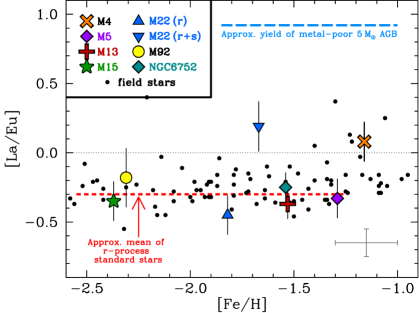
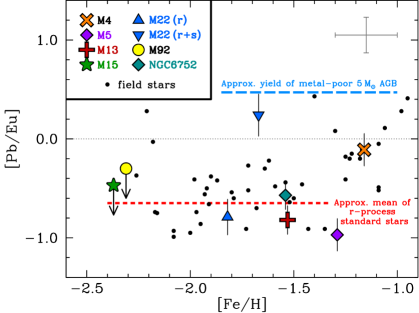
Figure 5.— [La/Eu] and [Pb/Eu] ratios as a function of [Fe/H]. Only GCs where Pb has been measured have been included. The dotted lines indicate the solar ratio. A typical uncertainty is shown. The blue long-dashed lines indicate the approximate yields of a 5 $M_{\odot}$ AGB star at [Fe/H] $=-$2.3 (Roederer et al., 2010b). The red short-dashed lines indicate the approximate means of metal-poor field stars whose [Pb/Eu] ratios are consistent with having been enriched by $r$-process material only (Roederer et al., 2010b). GC abundances are referenced as follows: M4 and M5, Yong et al. (2008a, b); M13 and NGC 6752, Yong et al. (2006); M15, Sobeck et al. (2011); M92, Roederer & Sneden (2011); M22, this study; field stars, Roederer et al. (2010b). All abundances have been normalized to the scale used in the present study.

Table 6Mean Abundances in the $r$ and $r+s$ Groups

		$r$-only			$r+s$
Species	$Z$	$\langle$[X/Fe]$\rangle$	$\sigma_{\mu}$		$\langle$[X/Fe]$\rangle$	$\sigma_{\mu}$
Na i	11	0.08	0.018		0.49	0.023
Mg i	12	0.39	0.064		0.45	0.060
Al i	13	0.34	0.034		0.69	0.036
Si i	14	0.14	0.064		0.33	0.044
K i	19	0.80	0.064		0.90	0.064
Ca i	20	0.40	0.023		0.48	0.019
Sc ii	21	0.21	0.073		0.30	0.077
Ti i	22	0.06	0.015		0.07	0.028
Ti ii	22	0.47	0.020		0.45	0.026
V i	23	$-$0.14	0.026		$-$0.10	0.035
Cr i	24	$-$0.14	0.020		$-$0.17	0.019
Cr ii	24	0.14	0.064		0.24	0.064
Mn i	25	$-$0.50	0.034		$-$0.53	0.034
Fe i	26	$-$1.81	0.008		$-$1.81	0.009
Fe ii	26	$-$1.78	0.022		$-$1.78	0.028
Co i	27	$-$0.15	0.033		$-$0.03	0.027
Ni i	28	$-$0.20	0.020		$-$0.15	0.016
Cu i	29	$-$0.66	0.033		$-$0.49	0.033
Zn i	30	0.04	0.032		0.24	0.039
Rb i	37	$<$0.20	$\cdots$		$<$0.49	$\cdots$
Sr i	38	$-$0.53	0.064		$-$0.01	0.064
Y ii	39	$-$0.24	0.013		0.29	0.014
Zr i	40	$-$0.08	0.036		0.34	0.035
Zr ii	40	0.22	0.030		0.55	0.034
Mo i	42	0.11	0.078		0.12	0.111
Ru i	44	0.13	0.053		0.28	0.044
Rh i	45	$-$0.30	0.078		0.14	0.072
Ba ii	56	0.18	0.047		0.74	0.033
La ii	57	0.08	0.016		0.51	0.013
Ce ii	58	$-$0.07	0.009		0.49	0.017
Pr ii	59	0.12	0.016		0.42	0.017
Nd ii	60	0.15	0.009		0.52	0.011
Sm ii	62	0.27	0.013		0.46	0.018
Eu ii	63	0.35	0.056		0.32	0.046
Gd ii	64	0.33	0.043		0.51	0.046
Tb ii	65	$-$0.05	0.064		0.18	0.078
Dy ii	66	0.42	0.036		0.51	0.029
Ho ii	67	0.12	0.115		0.12	0.115
Er ii	68	0.38	0.033		0.52	0.063
Tm ii	69	0.09	0.045		0.19	0.200
Yb ii	70	$-$0.11	0.115		0.25	0.064
Hf ii	72	$-$0.11	0.064		0.36	0.064
Ir i	77	0.45	0.064		$\cdots$	$\cdots$
Pb i	82	$-$0.26	0.064		0.56	0.064
Th ii	90	0.21	0.064		$\cdots$	$\cdots$

Note. — The means represent weighted means from the 3 stars in each group, and the stated uncertainties represent internal uncertainties only. $\langle$[Fe/H]$\rangle$ is listed in the $\langle$[X/Fe]$\rangle$ column for Fe i and Fe ii.

5. Comparison to Other Complex Metal-poor GCs

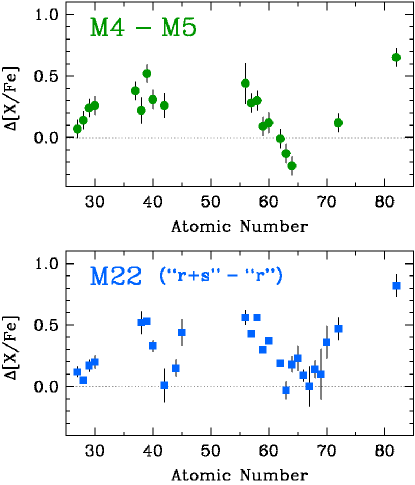
Figure 6.— Top panel: Differences between the mean abundances in GCs M4 and M5. The abundances are taken from Yong et al. (2008a, b) and Ivans et al. (1999, 2001). Bottom panel: Differences between the mean abundances in the $r+s$ and $r$ groups in M22. In both panels, dotted lines indicate zero difference.

Table 7Mean Line-by-line Differentials for K–Zn in the $r$ and $r+s$ Groups

Species	$N$	$\langle\Delta$[X/Fe]$\rangle$	$\sigma$	$\sigma_{\mu}$
K i	1	$+$0.100	0.090	0.090
Ca i	8	$+$0.066	0.063	0.022
Sc ii	5	$+$0.087	0.048	0.022
Ti i	9	$-$0.007	0.087	0.029
Ti ii	9	$-$0.003	0.062	0.021
Ti i$+$ii	18	$-$0.005	0.073	0.017
V i	5	$+$0.057	0.060	0.027
Cr i	6	$-$0.016	0.073	0.030
Cr ii	1	$+$0.105	0.110	0.110
Cr i$+$ii	7	$-$0.008	0.085	0.032
Mn i	4	$-$0.064	0.078	0.039
Co i	4	$+$0.094	0.065	0.033
Ni i	10	$+$0.029	0.073	0.023
Cu i	2	$+$0.169	0.088	0.062
Zn i	2	$+$0.189	0.052	0.036

As discussed in Marino et al. (2009, 2011b), evidence for multiple stellar populations in M22 includes the following: (1) the SGB shows two distinct sequences, (2) there is a metallicity offset between the two groups, (3) each group independently exhibits the O–Na and C–N anticorrelations, and (4) there are clearly distinct $n$-capture abundance patterns in the two groups. It is difficult to envision an unambiguous evolutionary picture for M22 that accounts for the entire body of observations. Here, we illuminate this issue by comparing M22 with other GCs that show similar complexity, like NGC 1851, and simpler GCs, like M4 and M5.

The GCs M4 and M5 are a frequently studied pair of clusters that are not physically related to one another. Both are more metal-rich than M22 ([Fe/H] $=-$1.2 and $-$1.3), and previous work has revealed that M4 contains moderate $s$-process enrichment relative to M5 (Ivans et al., 1999, 2001; Yong et al., 2008a, b; Marino et al., 2008). The heavy element abundances in M5 are similar to the scaled S.S. $r$-process residuals (Yong et al., 2008a, b; Lai et al., 2011), and the low Pb abundance (Yong et al., 2008a) suggests that these elements were produced by $r$-process nucleosynthesis without the need to invoke contributions from the $s$-process (Roederer et al., 2010b; Roederer, 2011). We subtract the heavy element abundances in M5 from those in M4 (cf. Yong et al. 2008b) to estimate the $s$-process contribution to M4. As shown in Figure 6, these differences are remarkably similar to the differences observed between the $r+s$ and $r$-only groups in M22. There is a gradual increase in the $s$-process content of Co through Zn (27 $\leq Z\leq$ 30), a moderate $s$-process contribution with some element-to-element scatter for Rb–Rh (37 $\leq Z\leq$ 45), a gradual decrease from Ba to Gd (56 $\leq Z\leq$ 64), and a gradual increase from Yb to Pb (70 $\leq Z\leq$ 82). There is no a priori reason to expect such similarity. Figure 6 implies that the heavy elements in M5 and the M22 $r$-only group were produced by similar nucleosynthesis mechanisms, and the heavy elements in M4 and the M22 $r+s$ group were produced by another similar set of nucleosynthesis mechanisms.

The heavy elements in NGC 1851 resemble the pattern observed in M22 (Yong & Grundahl, 2008; Yong et al., 2009; Carretta et al., 2010, 2011), and Carretta et al. raised the possibility that NGC 1851 may have formed through the merger of two proto-clusters in a now dissolved dwarf galaxy. The Eu abundance within each of M22 and NGC 1851 is constant, but moderate enhancements are observed in Zr, Ba, La, and Ce in some stars of both GCs. Carretta et al. report a small but detectable spread in Fe and Ca in NGC 1851. Unlike M22, these two elements are strongly correlated, which implies the more metal-rich group is not enhanced in [Ca/Fe] relative to the metal-poor group. Note, however, that Lee et al. (2009) suggest much larger [Ca/H] variations are present in NGC 1851. Like M22, NGC 1851 has a split SGB (Milone et al., 2008), which may be explained by either an age difference of $\sim$ 1 Gyr or a difference in the overall CNO with a negligible age difference (Cassisi et al., 2008; Ventura et al., 2009). Examination of the radial distributions of different SGB populations gives conflicting results for NGC 1851, and radial distributions for the two groups of stars in M22 have not been investigated.

Table 8$r$- and $s$-process Percentages in the M22 $r+s$ Group

Element	$Z$	$N_{r+s}$	$N_{r}$	$N_{s}$	$\log\epsilon_{r+s}$	$\log\epsilon_{r}$	$\log\epsilon_{s}$	%$r$	%$s$	$\sigma_{\%s}$
Co	27	43.7	33.1	10.5	3.18	3.06	2.56	$\cdots$	24.1	${}^{+11.2}_{-9.8}$
Ni	28	562.	501.	61.2	4.29	4.24	3.33	$\cdots$	10.9	${}^{+7.7}_{-7.1}$
Cu	29	2.40	1.62	0.777	1.92	1.75	1.43	$\cdots$	32.4	${}^{+11.1}_{-9.5}$
Zn	30	30.2	19.1	11.1	3.02	2.82	2.59	$\cdots$	36.9	${}^{+11.2}_{-9.5}$
Sr	38	0.347	0.105	0.242	1.08	0.56	0.92	30.2	69.8	${}^{+10.4}_{-7.7}$
Y	39	0.151	0.0447	0.107	0.72	0.19	0.57	29.5	70.5	${}^{+1.9}_{-1.8}$
Zr (i)	40	0.347	0.151	0.247	1.14	0.72	0.93	38.0	62.0	${}^{+6.8}_{-5.7}$
Zr (ii)	40	0.646	0.302	0.344	1.35	1.02	1.08	46.8	53.2	${}^{+7.4}_{-6.4}$
Mo	42	0.0479	0.0468	0.00109	0.22	0.21	$-$1.42	97.7	2.3	${}^{+53.3}_{-2.3}$
Ru	44	0.0513	0.0363	0.0150	0.25	0.10	$-$0.28	70.8	29.2	${}^{+17.7}_{-14.2}$
Rh	45	0.00759	0.00275	0.00483	$-$0.58	$-$1.02	$-$0.78	36.3	63.7	${}^{+15.0}_{-10.6}$
Ba	56	0.398	0.110	0.288	1.14	0.58	1.00	27.5	72.5	${}^{+5.6}_{-4.6}$
La	57	0.0195	0.00724	0.0122	$-$0.17	$-$0.60	$-$0.37	37.2	62.8	${}^{+2.6}_{-2.4}$
Ce	58	0.0562	0.0155	0.0408	0.29	$-$0.27	0.15	27.5	72.5	${}^{+1.7}_{-1.6}$
Pr	59	0.00661	0.00331	0.00330	$-$0.64	$-$0.94	$-$0.94	50.1	49.9	${}^{+4.0}_{-3.7}$
Nd	60	0.0417	0.0178	0.0239	0.16	$-$0.21	$-$0.08	42.7	57.3	${}^{+2.0}_{-1.9}$
Sm	62	0.0126	0.00813	0.00446	$-$0.36	$-$0.55	$-$0.81	64.6	35.4	${}^{+4.8}_{-4.4}$
Eu	63	0.00331	0.00355	$-$0.000237	$-$0.94	$-$0.91	$\cdots$	100.	0.0	${}^{+28.4}_{-0.0}$
Gd	64	0.0182	0.0120	0.00617	$-$0.20	$-$0.38	$-$0.67	66.1	33.9	${}^{+15.0}_{-12.2}$
Tb	65	0.00145	0.000851	0.000594	$-$1.30	$-$1.53	$-$1.69	58.9	41.1	${}^{+22.8}_{-16.4}$
Dy	66	0.0195	0.0158	0.00365	$-$0.17	$-$0.26	$-$0.90	81.3	18.7	${}^{+13.1}_{-11.3}$
Ho	67	0.00191	0.00191	0.00	$-$1.18	$-$1.18	$\cdots$	100.	0.0	${}^{+69.8}_{-0.0}$
Er	68	0.0132	0.00955	0.00363	$-$0.34	$-$0.48	$-$0.90	72.4	27.6	${}^{+17.9}_{-14.4}$
Tm	69	0.000933	0.000741	0.000192	$-$1.49	$-$1.59	$-$2.18	79.4	20.6	${}^{+60.2}_{-20.6}$
Yb	70	0.00708	0.00309	0.00399	$-$0.61	$-$0.97	$-$0.86	43.7	56.3	${}^{+22.3}_{-14.7}$
Hf	72	0.00776	0.00263	0.00513	$-$0.57	$-$1.04	$-$0.75	33.9	66.1	${}^{+11.6}_{-8.6}$
Ir	77	$\cdots$	0.0324	$\cdots$	$\cdots$	0.05	$\cdots$	$\cdots$	$\cdots$	$\cdots$
Pb	82	0.191	0.0288	0.162	0.82	0.00	0.75	15.1	84.9	${}^{+5.2}_{-3.9}$
Th	90	$\cdots$	0.000891	$\cdots$	$\cdots$	$-$1.51	$\cdots$	$\cdots$	$\cdots$	$\cdots$

The M22 chemistry does not exclude the possibility that it formed through a merger of two separate groups similar to M4 and M5 (at lower metallicity). The $s$-process abundances in the two M22 groups are sufficiently distinct that these two groups would be regarded as completely separate populations if not observed together in the same GC. Similar metallicities and $r$-process abundances might be expected if the groups formed in close proximity in a now-dissolved dwarf galaxy.

On the other hand, M22 shares several characteristics with the metal-poor populations in $\omega$ Cen, which is more difficult to interpret as having formed via merging of several clusters. Based on current self-enrichment models, a possible way to account for the M22 chemistry is through fine-tuning of the times of accumulation of the material from which successive generations form. In this scenario M22 does not evolve as an isolated system, and external gas flows can contribute to the enrichment processes (Marino et al., 2011b). A similar mechanism has been recently suggested by D’Antona et al. (2011) to explain the O–Na anticorrelation pattern in the more complex case of $\omega$ Cen (Johnson & Pilachowski, 2010; Marino et al., 2011a). Further exploration is beyond the scope of the present work.

6. The Source of the $s$-process Material

To summarize the results of the previous sections, the heavy elements in the M22 $r$-only group can be explained by nucleosynthesis mechanisms associated with core collapse SNe. The $r+s$ group contains a moderate amount of material produced by $s$-process nucleosynthesis. Previous studies have shown that the $r+s$ group has a higher mean metallicity than the $r$-only group, but the ratio of $r$-process material to Fe-group material is roughly equal in the two groups. In this section we investigate possible nucleosynthetic sources for the $s$-process material in the $r+s$ group.

We subtract the $r$-process contribution (i.e., the abundance in the $r$-only group) to each of La and Pb in the $r+s$ group to derive the intrinsic [Pb/La]_s ratio. We perform a similar calculation to estimate the intrinsic $s$-process ratios in M4 by subtracting the M5 abundances using the Yong et al. (2008a) abundances. This yields [Pb/La]${}_{s}=+$0.18 $\pm$ 0.09 in M22 and [Pb/La]${}_{s}=-$0.01 $\pm$ 0.08 in M4. Similarly, we derive the indices [$hs$/$ls$]${}_{s}=-$0.01 and $-$0.50 and [Pb/$hs$] $=+$0.29 and $+$0.28 for M22 and M4, respectively. (Uncertainties on each of these quantities are likely 0.10–0.15 dex.) These ratios and indices are useful since they are insensitive to the dredge-up efficiency or the dilution of AGB products in the stars currently observed. We infer that the AGBs providing the $s$-process enrichment in M4 and the $r+s$ group in M22 were similar but not identical.

Models of $s$-process nucleosynthesis indicate that Pb is a sensitive probe of the stellar mass, metallicity, and neutron flux. Goriely & Mowlavi (2000) present yields for a model representative of 1.5 $\leq M\leq$ 3.0 $M_{\odot}$, [Fe/H] $=-$1.25 AGB stars, and [Pb/La] can be estimated from Figure 3 of Goriely & Siess (2001) for their 3 $M_{\odot}$ zero-metallicity AGB model. Cristallo et al. (2009) present yields for 2 $M_{\odot}$ AGB models at [Fe/H] $=-$1.2 and $-$2.2. Bisterzo et al. (2010) present a set of yields for several masses ($M=$ 1.3, 1.4, 1.5, and 2.0 $M_{\odot}$), metallicities ($-$3.6 $\leq$ [Fe/H] $\leq-$1.0), and ¹³C pocket efficiencies. [Pb/La] predictions can also be calculated for limited combinations of masses, metallicities, and ¹³C pocket efficiencies from the AGB yields presented in Roederer et al. (2010b). These predictions rely on similar atomic data, stellar models, assumptions about branching points, etc., and so are not entirely independent.

When compared with these yields, the M4 and M22 $s$-process heavy element ratios and indices point to a common theme: low mass AGB stars ($M\leq$ 3 $M_{\odot}$) cannot reproduce the observed values unless the standard ¹³C pocket efficiency is reduced by factors of 30–150. Pb is enhanced in both M4 and the $r+s$ group in M22 relative to the lighter $n$-capture elements and Fe, but it is not nearly as enhanced as observed in metal-poor stars extrinsically enriched in $s$-process elements by an AGB binary companion. AGBs with $M\sim$ 4.5–6.0 $M_{\odot}$ (those which may not form a ¹³C pocket and hence will not activate the ¹³C($\alpha$,$n$)¹⁶O neutron source) can produce lower [Pb/La] ratios (Roederer et al., 2010b). For comparison, predictions for the 5 $M_{\odot}$ AGB models at [Fe/H] $=-$2.3 are shown in Figure 5. Figures in Bisterzo et al. (2010) present the [$hs$/$ls$] and [Pb/$hs$] indices for a limited number of 3 and 5 $M_{\odot}$ AGB models. Their predictions for the appropriate (low) ¹³C pocket efficiency in a 5 $M_{\odot}$ AGB are a near-perfect match to the $s$-process ratios in each of M4 and M22 at their respective metallicities. This result is encouraging.

The ²²Ne neutron source, which activates at higher temperatures than the ¹³C neutron source, does not play a dominant role in AGB stars with $M<$ 3–4 $M_{\odot}$. In AGB stars with $M=$ 5–8 $M_{\odot}$, the temperature at the base of the thermal pulse is higher, and the ²²Ne($\alpha$,$n$)²⁵Mg reaction can occur there (e.g., Busso et al. 2001). In principle this could also account for the $s$-process neutron captures that produce small amounts of Co–Zn, as observed; see Yong et al. (2008b) and Karakas et al. (2009) for further discussion.

Models of the weak component of the $s$-process have traditionally been set in $\sim$ 25 $M_{\odot}$ stars (e.g., Raiteri et al. 1993) that activate the ²²Ne neutron source during core He-burning and shell C-burning stages, since models of less massive stars suggest that subsequent burning stages will destroy any $s$-process material created. Models that include rotationally-induced mixing can increase the neutron flux by mixing ¹⁴N (which is converted to ²²Ne) into the relevant regions, possibly producing nuclei as heavy as ²⁰⁸Pb (Pignatari et al., 2008). Yet the enhanced $s$-process abundances observed in the M22 $r+s$ group cannot be due to the operation of the weak $s$-process in massive stars. There is no reason to expect that the the SNe that enriched the metal-rich $r+s$ group in M22 host the weak $s$-process and those that enriched the metal-poor $r$-only group did not.

The minority neutron-rich Mg isotopes ²⁵Mg and ²⁶Mg may be produced (among other proton- and $\alpha$-capture channels) by the reaction sequence ²²Ne($\alpha$,$n$)²⁵Mg($n$,$\gamma$)²⁶Mg, which acts as both a neutron source and poison. Preliminary measurements of (²⁵Mg$+^{26}$Mg)/²⁴Mg in M4 and M5 indicate that the Mg isotopes have similar proportions in the two clusters (Yong et al., 2008b). While preliminary, these measurements hint that the source affecting the Mg isotopic ratios has acted similarly in M4 and M5. Since moderate quantities of $s$-process material are observed in M4 and M22 but not M5, it seems unlikely that the source of the $s$-process material modifies the Mg isotopic ratios substantially. Unfortunately we cannot assess the Mg isotopic ratios from our M22 data, but new measurements of these ratios in all three GCs would be of great interest.

At low metallicity ²²Ne also serves as a primary seed nucleus from which a chain of $n$-capture reactions can generate a small leakage across the Fe-group isotopes (Busso et al., 2001; Gallino et al., 2006). We propose that the observed variations in the Fe-group ratios and perhaps even the overall metallicity (Fe) increase in the $r+s$ group could be due to this phenomenon. The $s$-process path passes through stable or long-lived nuclei of K, Ca, Ti, V, and Cr, including several nuclei (³⁹K, ⁴²Ca, ⁴³Ca, ⁴⁴Ca, ⁵⁰Ti, ⁵¹V, ⁵²Cr) with closed nuclear shells. The only stable isotopes of Sc and Mn, ⁴⁵Sc and ⁵⁵Mn, do not have closed nuclear shells, so it is perhaps surprising that Sc shows an enhancement while Mn shows a deficiency in the $r+s$ group. The fact that we observe no change in Ti or Cr could be related to the initially larger abundances of these even-$Z$ elements relative to a small $s$-process contribution. Ca, which could also be expected to follow this pattern, may be enhanced because there are three Ca isotopes on the $s$-process path with closed proton shells. Obviously detailed calculations are needed to test these proposals for the Fe-group variations between the two groups in M22.

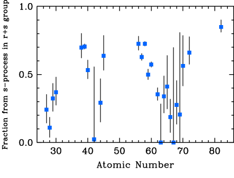
Figure 7.— The fractional component of the $r+s$ group of stars originating in the $s$-process for elements heavier than Fe.

If the $s$-process material in M4 and M22 is produced by neutrons from the ²²Ne source, this implies an origin different from that of the $s$-process material in $\omega$ Cen. Smith et al. (2000) found that the $n$-capture elements in $\omega$ Cen are best fit by low-mass (1.5–3.0 $M_{\odot}$) AGB stars where the ¹³C neutron source is active. The observed [Rb/Zr] ratios in $\omega$ Cen, which are quite sensitive to the neutron density and hence the neutron source because of $s$-process branching at ⁸⁵Kr, are best fit by low mass ($M\leq$ 3 $M_{\odot}$) AGB models. The [Rb/Zr] ratios in M4 derived by Yong et al. (2008a) are higher than those in $\omega$ Cen, and our [Rb/Zr] ratio in the M22 $r+s$ group is not lower than that in M4, supporting our assertion. (Recall that we could only derive upper limits on the Rb abundance in M22.) Furthermore, Cunha et al. (2002) found no evolution in the [Cu/Fe] ratio over $-$2.0 $<$ [Fe/H] $<-$0.8 in $\omega$ Cen, indicating that there were no contributions to Cu from AGB stars that could produce Cu with neutrons from the ²²Ne($\alpha$,$n$)²⁵Mg reaction. D’Antona et al. (2011) point out that the timescales for establishing the light element variations and the $s$-process enrichement in $\omega$ Cen are discrepant, and this issue is not yet resolved.

These constraints raise an obvious question: if the $s$-process material in M4 and M22 is produced in more massive AGB stars, then why is $s$-process material not detected in every cluster where the light element variations are observed? Marino et al. (2008) showed that there might be a weak correlation between [Ba/Fe] and [Al/Fe] in M4, a point also investigated by Smith (2008). Those data also suggest weak correlations between [Ba/Fe] and each of [Na/Fe] and [Si/Fe]. For the majority of GCs, however, such correlations are not found (e.g., Armosky et al. 1994; D’Orazi et al. 2010). This supports our conclusion, drawn from the [Pb/Eu] ratios, that the heavy elements in most metal-poor GCs are produced by $r$-process nucleosynthesis. Perhaps in GCs like M4, the $r+s$ group in M22, or the metal-rich group of NGC 1851, material from slightly lower AGB masses was allowed to enrich the GC ISM before the clusters formed. This might suggest that these particular clusters were more massive initially or originated in dwarf galaxies whose potentials could more easily retain ejecta and sustain extended periods of star formation. This scenario is appealing because several of the metal-poor clusters exhibiting $s$-process enrichment (M22, NGC 1851, $\omega$ Cen) exhibit at least minimal spreads in Fe and (in the case of M22 and NGC 1851) could have been formed through mergers.

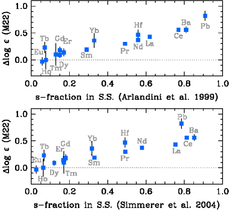
Figure 8.— Differences in the mean abundances between the $r$-only group and the $r+s$ group as a function of the $s$-fraction of each element in the S.S. The top panel shows the $s$-fraction as calculated from the average yields of the 1.5 and 3.0 $M_{\odot}$ stellar models at [Fe/H] $=-$0.3 of Arlandini et al. (1999), including the contribution of low-metallicity AGB stars to the S.S. Pb as derived by Travaglio et al. (2001). The bottom panel shows the $s$-fraction as calculated by the classical method (Simmerer et al., 2004). The dotted lines indicate zero difference.

In summary, the observed $s$-process abundance patterns are not well-fit by low-metallicity models of AGB stars with $M\leq$ 3 $M_{\odot}$. Higher mass AGBs that activate the ²²Ne neutron source may provide a better fit. Both stellar groups in M22 exhibit the Na–O anticorrelation, but the observed lack of a correlation between $s$-process enrichment and Na within the $r+s$ group is difficult to understand if these elements are all produced by AGB stars of higher masses. We encourage more detailed exploration of the possible association between the $s$-process products in these metal-poor GCs with intermediate-mass AGB stars.

7. An Empirical $s$-process Abundance Distribution

In this section we compare the nature of low-metallicity $s$-process enrichment with the $s$-process abundance pattern observed in the S.S. The M22 $s$-process “residual” is derived by subtracting the abundances in the $r$-only group from the abundances in the $r+s$ group. This method assumes that the $r$-process material in both groups is identical, as indicated by observations.

Table 8 lists the abundances and $r$- and $s$-process fractions for the heavy elements in M22. Figure 7 illustrates the fraction of each of these elements that originates in the $s$-process in the M22 $r+s$ group. Elements on the $s$-process path with closed neutron shells (Sr–Zr, Ba–Nd, and Pb), plus a few others (Rh, Yb, Hf), owe more than 50% of their abundance in the $r+s$ group to the $s$-process. Elements in the middle of the rare earth domain (Sm–Tm) and just beyond the first $s$-process peak (Mo, Ru) are still mostly made of $r$-process material, with $s$-process fractions less than 40% or so. More than 80% of the Pb in the $r+s$ group originated in the $s$-process, the most of any element studied. Several elements, including Mo, Eu, Ho, and Tm, are consistent with a pure $r$-process origin (i.e., show no enhancement in the $r+s$ group) within the uncertainties. In analogy with S.S. $r$-residuals derived via the classical approach, elements with small $s$-process fractions have the largest $s$-process fraction uncertainties, and elements with large $s$-process fractions have the smallest uncertainties.

To compare the $s$-process fractions in M22 with the $s$-process fractions derived from the stellar model and classical approach, Figure 8 displays the elemental abundance differences between the two M22 groups as a function of the $s$-process fraction in the S.S. Only elements produced predominantly by the main and strong $s$-process components in the S.S. are shown (i.e., $Z\geq$ 56), since the yields of these elements should be less sensitive to the source of the neutron flux. There is a remarkably clear correlation, which changes little when different stellar model $s$-process fractions (e.g., Arlandini et al. 1999; Bisterzo et al. 2010) or classical method $s$-process fractions (e.g., Burris et al. 2000; Simmerer et al. 2004) are used. Note that the $s$-process fraction of Pb shown in Figure 8 accounts for the low-metallicity AGB component according to the Galactic chemical evolution model of Travaglio et al. (2001). The stellar model of Gallino et al. (1998) and Arlandini et al. (1999) designated the standard case for the mass of the ¹³C pocket as that which best reproduced the S.S. main $s$-process component in low-mass (1.5 and 3.0 $M_{\odot}$) AGB models with [Fe/H] $=-$0.3. The $s$-process material in the S.S. was produced by a variety of AGB sources over many Gyr. Despite this fact, Figure 8 suggests that—at least for the elements with 56 $\leq Z\leq$ 72—the relative yields of low-metallicity, higher-mass AGB stars are not that different from the more metal-rich, lower-mass AGB stars.

In the M22 $r+s$ group, 62% of the total amount of $Z\geq$ 38 elements examined (excluding Ir and Th) originated in the $s$-process. The $s$-process contributes 79% of the material to these same elements in the S.S. (Sneden et al., 2008). Hypothetically, if one wants to further enrich the heavy elements in the M22 $r+s$ group to match the S.S. abundances, a greater fraction of $s$-process material (with respect to $r$-process material) needs to be added. In principle, then, these data support the general understanding that $s$-process enrichment occurs at later times than $r$-process enrichment.

8. Conclusions

One longstanding obstacle to properly interpret models of the $s$-process is having observations of pure $s$-process material outside the S.S. to compare with, especially since nearly all stars contain at least a trace of $r$-process material. Here we provide one solution to this problem by deriving the abundance patterns in two related groups of stars in the metal-poor GC M22. One group shows an $r$-process pattern with no detectable enrichment by $s$-process material (the $r$-only group), while the other group shows an additional $s$-process enhancement (the $r+s$ group). By subtracting the $r$-process abundance pattern of the former from the $r+s$ abundance pattern in the latter, we explicitly remove the $r$-process contribution to reveal the $s$-process “residual.”

The $s$-process abundance pattern in M22 strongly disfavors low mass ($M\leq$ 3 $M_{\odot}$), low-metallicity AGB models. Although no published model results span the appropriate range of AGB masses at the metallicity of M22, the limited predictions available for more massive AGB stars at low metallicity fit the data better, especially the moderate Pb enhancement. Predictions for $M=$ 4.5 and 5.0 $M_{\odot}$ AGB models at [Fe/H] $=-$1.6 and $-$2.3 do fit the M22 $s$-process abundances, although 3 $<M<$ 4.5 $M_{\odot}$ models cannot be excluded because no predictions are available. The neutrons that fuel the $s$-process in these models mainly originate in the ²²Ne($\alpha$,$n$)²⁵Mg reaction, which requires higher activation temperatures than the ¹³C($\alpha$,$n$)¹⁶O reaction. In principle this could explain observed overabundances of K, Ca, Sc, V, Co, Ni, Cu, and Zn in the $r+s$ group. We also calculate the $r$- and $s$-process fractions of each $n$-capture element. This approach assumes nothing about the $r$- and $s$-process fractions in S.S. material. We encourage investigations of $s$-process nucleosynthesis in models with the appropriate metallicity and AGB mass range to better understand the origin of the heavy elements in M22. More generally, we hope that these data will serve as useful benchmarks for modeling and interpreting $s$-process abundance patterns and enrichment in low metallicity environments.

Furthermore, these abundances can help interpret the enrichment history of M22. The $Z\geq$ 27 abundance pattern in the M22 $r$-only and $r+s$ groups bear striking resemblance to the (physically unrelated) GCs M5 and M4, respectively. The $r+s$ group in M22 may share a similar enrichment history to M4 and possibly the metal-rich group in NGC 1851. If the $s$-process in M22 did originate in more massive AGB stars, this places strong constraints on the timescale for chemical enrichment, particularly in attempting to explain why the majority of metal-poor GCs do not show similar signatures of $s$-process enrichment. AGB models that can simultaneously explain the observed abundance patterns resulting from both proton- and neutron-capture reactions (the light element variations and $s$-process enrichment) should prove enlightening in this regard.

Appendix A Line-by-Line Mean Offsets

Table 9Line-by-line Mean Offsets

Species	$\lambda$ (Å)	$\langle\Delta\rangle$	$\sigma$	$\sigma_{\mu}$	Species	$\lambda$ (Å)	$\langle\Delta\rangle$	$\sigma$	$\sigma_{\mu}$
Y ii	4883.68	$-$0.009	0.081	0.033	Nd ii	4021.33	$-$0.081	0.108	0.022
Y ii	4982.13	$-$0.003	0.086	0.035	Nd ii	4059.95	$-$0.095	0.144	0.029
Y ii	5087.42	0.005	0.076	0.031	Nd ii	4232.37	$-$0.034	0.074	0.015
Y ii	5119.11	0.007	0.046	0.019	Nd ii	4446.38	$-$0.013	0.051	0.010
Y ii	5200.41	$-$0.003	0.051	0.021	Nd ii	4462.98	0.216	0.227	0.046
Y ii	5205.73	0.034	0.045	0.018	Nd ii	4465.06	0.054	0.067	0.014
Y ii	5289.82	$-$0.032	0.095	0.039	Nd ii	4465.59	$-$0.006	0.051	0.010
Zr ii	4050.33	$-$0.200	0.230	0.163	Nd ii	4501.81	0.020	0.069	0.014
Zr ii	4613.92	0.145	0.180	0.127	Nd ii	4567.61	0.002	0.048	0.010
Zr ii	5112.28	0.055	0.066	0.047	Nd ii	4645.76	$-$0.012	0.048	0.010
La ii	3988.51	$-$0.216	0.230	0.064	Nd ii	4706.54	0.068	0.075	0.015
La ii	3995.74	$-$0.115	0.185	0.051	Nd ii	4797.15	$-$0.098	0.141	0.029
La ii	4086.71	$-$0.076	0.130	0.036	Nd ii	4825.48	0.007	0.041	0.008
La ii	4322.50	$-$0.085	0.098	0.027	Nd ii	4859.03	0.023	0.042	0.009
La ii	4662.50	0.000	0.031	0.009	Nd ii	4902.04	0.084	0.091	0.019
La ii	4748.73	$-$0.083	0.093	0.026	Nd ii	4914.38	$-$0.008	0.023	0.005
La ii	4804.04	0.068	0.074	0.021	Nd ii	5089.83	$\equiv$0.0	0.065	0.013
La ii	4920.98	0.161	0.172	0.048	Nd ii	5092.79	$-$0.024	0.059	0.012
La ii	4986.82	0.034	0.071	0.020	Nd ii	5130.59	$-$0.059	0.073	0.015
La ii	5114.56	0.089	0.100	0.028	Nd ii	5132.33	$-$0.055	0.102	0.021
La ii	5290.84	$-$0.074	0.097	0.027	Nd ii	5234.19	$-$0.034	0.047	0.010
La ii	5303.53	0.068	0.092	0.026	Nd ii	5249.58	0.070	0.083	0.017
La ii	6262.29	0.093	0.100	0.028	Nd ii	5255.51	$-$0.006	0.038	0.008
La ii	6390.48	0.136	0.145	0.040	Nd ii	5293.16	$-$0.052	0.090	0.018
La ii	6774.27	$\equiv$0.0	0.075	0.021	Nd ii	5319.81	0.035	0.047	0.010
Ce ii	4073.47	$-$0.082	0.108	0.028	Sm ii	4318.93	$-$0.034	0.067	0.024
Ce ii	4083.22	0.046	0.087	0.023	Sm ii	4434.32	0.053	0.083	0.029
Ce ii	4120.83	0.043	0.056	0.014	Sm ii	4467.34	$-$0.124	0.137	0.048
Ce ii	4127.36	$-$0.180	0.204	0.053	Sm ii	4536.51	0.038	0.055	0.019
Ce ii	4137.65	$-$0.053	0.146	0.038	Sm ii	4537.94	$-$0.086	0.091	0.032
Ce ii	4222.60	0.027	0.100	0.026	Sm ii	4591.81	0.023	0.086	0.030
Ce ii	4364.65	$-$0.073	0.100	0.026	Sm ii	4642.23	0.075	0.089	0.031
Ce ii	4418.78	0.041	0.056	0.014	Sm ii	4669.64	$-$0.041	0.061	0.022
Ce ii	4486.91	$-$0.023	0.112	0.029	Sm ii	4719.84	0.096	0.110	0.039
Ce ii	4560.96	0.016	0.045	0.012	Eu ii	3907.11	$-$0.246	0.252	0.178
Ce ii	4562.36	0.016	0.046	0.012	Eu ii	4129.72	0.009	0.087	0.062
Ce ii	4572.28	0.037	0.075	0.019	Eu ii	6645.06	0.237	0.258	0.182
Ce ii	4582.50	0.055	0.095	0.025	Gd ii	4130.37	0.173	0.190	0.134
Ce ii	4628.16	0.089	0.102	0.026	Gd ii	4251.73	$-$0.097	0.152	0.108
Ce ii	5274.23	0.032	0.063	0.016	Gd ii	4498.29	$-$0.076	0.127	0.090
Ce ii	5330.56	0.011	0.087	0.022	Dy ii	3694.81	$-$0.108	0.321	0.185
Pr ii	4222.95	0.012	0.041	0.024	Dy ii	3983.65	0.073	0.120	0.069
Pr ii	4408.81	$-$0.041	0.050	0.029	Dy ii	4073.12	$-$0.078	0.153	0.088
Pr ii	5259.73	0.012	0.051	0.030	Dy ii	4449.70	0.113	0.161	0.093
Pr ii	5322.77	0.017	0.024	0.014

Note. — For a given line, the mean offset $\langle\Delta\rangle$ is computed as the average over all 6 stars of the offset relative to the mean of all other lines of the same species in a given star. Exceptions are Gd ii, whose mean is computed without I-80, and Dy ii, whose mean is computed without I-27 and I-80.

We have calculated line-by-line mean offsets for $n$-capture species whose abundance is derived from three or more lines. Such information is useful when comparing abundances from different studies that use a small number of non-overlapping lines. In Table 9, we list the species (columns 1 and 6), wavelength (columns 2 and 7), average offset from the mean abundance as derived for each of the 6 stars examined (columns 3 and 8), standard deviation of the average offset (columns 4 and 9), and standard deviation of the mean of the average offset (columns 5 and 10).

Because the number of La ii and Nd ii lines examined is large, we have also derived empirical $\log(gf)$ values for two lines not covered in the Lawler et al. (2001a) and Den Hartog et al. (2003) laboratory studies, La ii 6774.27Å ($\log(gf)=-$1.77 $\pm$ 0.06) and Nd ii 5089.83Å ($\log(gf)=-$1.27 $\pm$ 0.06). These lines are not used in determining the abundances in M22. This La ii line is often one of the only lines available in studies that target the red region of the spectrum. Johnson & Pilachowski (2010) provide empirical corrections to the abundance to account for the unknown HFS pattern of this line. In the M22 stars observed, the EWs of this line are all 10–20 mÅ, so the correction is approximately zero.

References

- Arlandini et al. (1999) Arlandini, C., Käppeler, F., Wisshak, K., Gallino, R., Lugaro, M., Busso, M., & Straniero, O. 1999, ApJ, 525, 886
- Armosky et al. (1994) Armosky, B. J., Sneden, C., Langer, G. E., & Kraft, R. P. 1994, AJ, 108, 1364
- Barklem et al. (2005) Barklem, P. S., et al. 2005, A&A, 439, 129
- Beers et al. (1992) Beers, T. C., Preston, G. W., & Shectman, S. A. 1992, AJ, 103, 1987
- Bernstein et al. (2003) Bernstein, R., Shectman, S. A., Gunnels, S. M., Mochnacki, S., & Athey, A. E. 2003, Proc. SPIE, 4841, 1694
- Bielski (1975) Bielski, A. 1975, J. Quant. Spec. Radiat. Transf., 15, 463
- Biémont & Godefroid (1980) Biémont, E., & Godefroid, M. 1980, A&A, 84, 361
- Biémont et al. (1981) Biémont, E., Grevesse, N., Hannaford, P., & Lowe, R. M. 1981, ApJ, 248, 867
- Biémont et al. (2000) Biémont, E., Garnir, H. P., Palmeri, P., Li, Z. S., & Svanberg, S. 2000, MNRAS, 312, 116
- Bisterzo et al. (2009) Bisterzo, S., Gallino, R., Straniero, O., & Aoki, W. 2009, Publ. Astron. Soc. Australia, 26, 314
- Bisterzo et al. (2010) Bisterzo, S., Gallino, R., Straniero, O., Cristallo, S., Käppeler, F. 2010, MNRAS, 404, 1529
- Bisterzo et al. (2011) Bisterzo, S., Gallino, R., Straniero, O., Cristallo, S., & Kaeppeler, F. 2011, MNRAS, in press (arXiv:1108.0500)
- Blackwell et al. (1982a) Blackwell, D. E., Petford, A. D., Shallis, M. J., & Leggett, S. 1982a, MNRAS, 199, 21
- Blackwell et al. (1982b) Blackwell, D. E., Menon, S. L. R., Petford, A. D., & Shallis, M. J. 1982b, MNRAS, 201, 611
- Blackwell-Whitehead & Bergemann (2007) Blackwell-Whitehead, R., & Bergemann, M. 2007, A&A, 472, L43
- Booth et al. (1984) Booth, A. J., Blackwell, D. E., Petford, A. D., & Shallis, M. J. 1984, MNRAS, 208, 147
- B2FH (1957) Burbidge, E. M., Burbidge, G. R., Fowler, W. A., & Hoyle, F. 1957, Reviews of Modern Physics, 29, 547 (B2FH)
- Burris et al. (2000) Burris, D. L., Pilachowski, C. A., Armandroff, T. E., Sneden, C., Cowan, J. J., & Roe, H. 2000, ApJ, 544, 302
- Busso et al. (1999) Busso, M., Gallino, R., & Wasserburg, G. J. 1999, ARA&A, 37, 239
- Busso et al. (2001) Busso, M., Gallino, R., Lambert, D. L., Travaglio, C., & Smith, V. V. 2001, ApJ, 557, 802
- Cameron (1973) Cameron, A. G. W. 1973, Space Sci. Rev., 15, 121
- Cardon et al. (1982) Cardon, B. L., Smith, P. L., Scalo, J. M., & Testerman, L. 1982, ApJ, 260, 395
- Carretta et al. (2010) Carretta, E., et al. 2010, ApJ, 722, L1
- Carretta et al. (2011) Carretta, E., Lucatello, S., Gratton, R., Bragaglia, A., & D’Orazi, V. 2011, A&A, in press (arXiv:1106.3174)
- Cassisi et al. (2008) Cassisi, S., Salaris, M., Pietrinferni, A., Piotto, G., Milone, A. P., Bedin, L. R., & Anderson, J. 2008, ApJ, 672, L115
- Castelli & Kurucz (2004) Castelli, F., & Kurucz, R. L. Proc. IAU Symp. No 210, Modelling of Stellar Atmospheres, eds. N. Piskunov et al. 2003, A20 (arXiv:0405087)
- Chang & Tang (1990) Chang, T. N., & Tang, X. 1990, J. Quant. Spec. Radiat. Transf., 43, 207
- Clayton et al. (1961) Clayton, D. D., Fowler, W. A., Hull, T. E., & Zimmerman, B. A. 1961, Ann. Phys. 12, 331
- Clayton & Rassbach (1967) Clayton, D. D., & Rassbach, M. E. 1967, ApJ, 148, 69
- Clayton (1988) Clayton, D. D. 1988, MNRAS, 234, 1
- Cowan et al. (1995) Cowan, J. J., Burris, D. L., Sneden, C., McWilliam, A., & Preston, G. W. 1995, ApJ, 439, L51
- Cowan et al. (2002) Cowan, J. J., et al. 2002, ApJ, 572, 861
- Cowan et al. (2005) Cowan, J. J., et al. 2005, ApJ, 627, 238
- Cristallo et al. (2009) Cristallo, S., Straniero, O., Gallino, R., Piersanti, L., Domínguez, I., & Lederer, M. T. 2009, ApJ, 696, 797
- Cunha et al. (2002) Cunha, K., Smith, V. V., Suntzeff, N. B., Norris, J. E., Da Costa, G. S., & Plez, B. 2002, AJ, 124, 379
- D’Antona et al. (2011) D’Antona, F., D’Ercole, A., Marino, A. F., Milone, A. P., Ventura, P., & Vesperini, E. 2011, ApJ, 736, 5
- Den Hartog et al. (2003) Den Hartog, E. A., Lawler, J. E., Sneden, C., & Cowan, J. J. 2003, ApJS, 148, 543
- Den Hartog et al. (2006) Den Hartog, E. A., Lawler, J. E., Sneden, C., & Cowan, J. J. 2006, ApJS, 167, 292
- D’Orazi et al. (2010) D’Orazi, V., Gratton, R., Lucatello, S., Carretta, E., Bragaglia, A., & Marino, A. F. 2010, ApJ, 719, L213
- Duquette & Lawler (1985) Duquette, D. W., & Lawler, J. E. 1985, J. Opt. Soc. Am. B Optical Physics, 1, 1948
- Frebel et al. (2007) Frebel, A., Christlieb, N., Norris, J. E., Thom, C., Beers, T. C., & Rhee, J. 2007, ApJ, 660, L117
- Fuhr & Wiese (2009) Fuhr, J. R. & Wiese, W. L. 2005, Atomic Transition Probabilities, published in the CRC Handbook of Chemistry and Physics, 90th Edition, ed. Lide, D. R., CRC Press, Inc., Boca Raton, FL
- Gallino et al. (1998) Gallino, R., Arlandini, C., Busso, M., Lugaro, M., Travaglio, C., Straniero, O., Chieffi, A., & Limongi, M. 1998, ApJ, 497, 388
- Gallino et al. (2006) Gallino, R., Bisterzo, S., Husti, L., Käppeler, F., Cristallo, S., & Straniero, O. 2006, Proc. Internat. Symp. on Nucl. Astrophys., “Nuclei in the Cosmos IX,” 100, 1
- Goriely & Mowlavi (2000) Goriely, S., & Mowlavi, N. 2000, A&A, 362, 599
- Goriely & Siess (2001) Goriely, S., & Siess, L. 2001, A&A, 378, L25
- Grevesse et al. (1989) Grevesse, N., Blackwell, D. E., & Petford, A. D. 1989, A&A, 208, 157
- Gustafsson et al. (2008) Gustafsson, B., Edvardsson, B., Eriksson, K., Jørgensen, U. G., Nordlund, Å., & Plez, B. 2008, A&A, 486, 951
- Hannaford et al. (1982) Hannaford, P., Lowe, R. M., Grevesse, N., Biémont, E., & Whaling, W. 1982, ApJ, 261, 736
- Honda et al. (2007) Honda, S., Aoki, W., Ishimaru, Y., & Wanajo, S. 2007, ApJ, 666, 1189
- Ivans et al. (1999) Ivans, I. I., Sneden, C., Kraft, R. P., Suntzeff, N. B., Smith, V. V., Langer, G. E., & Fulbright, J. P. 1999, AJ, 118, 1273
- Ivans et al. (2001) Ivans, I. I., Kraft, R. P., Sneden, C., Smith, G. H., Rich, R. M., & Shetrone, M. 2001, AJ, 122, 1438
- Ivans et al. (2006) Ivans, I. I., Simmerer, J., Sneden, C., Lawler, J. E., Cowan, J. J., Gallino, R., & Bisterzo, S. 2006, ApJ, 645, 613
- Ivarsson et al. (2001) Ivarsson, S., Litzén, U., & Wahlgren, G. M. 2001, Phys. Scr, 64, 455
- Ivarsson et al. (2003) Ivarsson, S., et al. 2003, A&A, 409, 1141
- Johnson & Bolte (2001) Johnson, J. A., & Bolte, M. 2001, ApJ, 554, 888
- Johnson & Pilachowski (2010) Johnson, C. I., & Pilachowski, C. A. 2010, ApJ, 722, 1373
- Käppeler et al. (1989) Kappeler, F., Beer, H., & Wisshak, K. 1989, Reports on Progress in Physics, 52, 945
- Karakas et al. (2009) Karakas, A. I., van Raai, M. A., Lugaro, M., Sterling, N. C., & Dinerstein, H. L. 2009, ApJ, 690, 1130
- Kelson (2003) Kelson, D. D. 2003, PASP, 115, 688
- Kratz et al. (2007) Kratz, K.-L., Farouqi, K., Pfeiffer, B., Truran, J. W., Sneden, C., & Cowan, J. J. 2007, ApJ, 662, 39
- Kurucz & Bell (1995) Kurucz, R. L., & Bell, B. 1995, Kurucz CD-ROM, Cambridge, MA: Smithsonian Astrophysical Observatory
- Lai et al. (2011) Lai, D. K., Smith, G. H., Bolte, M., Johnson, J. A., Lucatello, S., Kraft, R. P., & Sneden, C. 2011, AJ, 141, 62
- Lambert et al. (1995) Lambert, D. L., Smith, V. V., Busso, M., Gallino, R., & Straniero, O. 1995, ApJ, 450, 302
- Lawler & Dakin (1989) Lawler, J. E., & Dakin, J. T. 1989, Journal of the Optical Society of America B Optical Physics, 6, 1457
- Lawler et al. (2001a) Lawler, J. E., Bonvallet, G., & Sneden, C. 2001a, ApJ, 556, 452
- Lawler et al. (2001b) Lawler, J. E., Wickliffe, M. E., den Hartog, E. A., & Sneden, C. 2001b, ApJ, 563, 1075
- Lawler et al. (2001c) Lawler, J. E., Wickliffe, M. E., Cowley, C. R., & Sneden, C. 2001c, ApJS, 137, 341
- Lawler et al. (2001d) Lawler, J. E., Wyart, J.-F., & Blaise, J. 2001d, ApJS, 137, 351
- Lawler et al. (2004) Lawler, J. E., Sneden, C., & Cowan, J. J. 2004, ApJ, 604, 850
- Lawler et al. (2006) Lawler, J. E., Den Hartog, E. A., Sneden, C., & Cowan, J. J. 2006, ApJS, 162, 227
- Lawler et al. (2007) Lawler, J. E., Den Hartog, E. A., Labby, Z. E., Sneden, C., Cowan, J. J., & Ivans, I. I. 2007, ApJS, 169, 120
- Lawler et al. (2008) Lawler, J. E., Sneden, C., Cowan, J. J., Wyart, J.-F., Ivans, I. I., Sobeck, J. S., Stockett, M. H., & Den Hartog, E. A. 2008, ApJS, 178, 71
- Lawler et al. (2009) Lawler, J. E., Sneden, C., Cowan, J. J., Ivans, I. I., & Den Hartog, E. A. 2009, ApJS, 182, 51
- Lee et al. (2009) Lee, J.-W., Lee, J., Kang, Y.-W., Lee, Y.-W., Han, S.-I., Joo, S.-J., Rey, S.-C., & Yong, D. 2009, ApJ, 695, L78
- Li et al. (2007) Li, R., Chatelain, R., Holt, R. A., Rehse, S. J., Rosner, S. D., & Scholl, T. J. 2007, Phys. Scr, 76, 577
- Ljung et al. (2006) Ljung, G., Nilsson, H., Asplund, M., & Johansson, S. 2006, A&A, 456, 1181
- Lodders (2003) Lodders, K. 2003, ApJ, 591, 1220
- Ludwig et al. (2010) Ludwig, H.-G., Caffau, E., Steffen, M., Bonifacio, P., & Sbordone, L. 2010, A&A, 509, A84
- Marín-Franch et al. (2009) Marín-Franch, A., et al. 2009, ApJ, 694, 1498
- Marino et al. (2008) Marino, A. F., Villanova, S., Piotto, G., Milone, A. P., Momany, Y., Bedin, L. R., & Medling, A. M. 2008, A&A, 490, 625
- Marino et al. (2009) Marino, A. F., Milone, A. P., Piotto, G., Villanova, S., Bedin, L. R., Bellini, A., & Renzini, A. 2009, A&A, 505, 1099
- Marino et al. (2011a) Marino, A. F., et al. 2011b, ApJ, 731, 64
- Marino et al. (2011b) Marino, A. F., et al. 2011b, A&A, 532, A8
- McWilliam (1998) McWilliam, A. 1998, AJ, 115, 1640
- Meléndez & Barbuy (2009) Meléndez, J., & Barbuy, B. 2009, A&A, 497, 611
- Migdalek & Baylis (1987) Migdalek, J., & Baylis, W. E. 1987, Canadian Journal of Physics, 65, 1612
- Milone et al. (2008) Milone, A. P., et al. 2008, ApJ, 673, 241
- Montes et al. (2007) Montes, F., et al. 2007, ApJ, 671, 1685
- Nilsson et al. (2002) Nilsson, H., Zhang, Z. G., Lundberg, H., Johansson, S., & Nordström, B. 2002, A&A, 382, 368
- Nilsson et al. (2006) Nilsson, H., Ljung, G., Lundberg, H., & Nielsen, K. E. 2006, A&A, 445, 1165
- Nitz et al. (1999) Nitz, D. E., Kunau, A. E., Wilson, K. L., & Lentz, L. R. 1999, ApJS, 122, 557
- O’Brian et al. (1991) O’Brian, T. R., Wickliffe, M. E., Lawler, J. E., Whaling, W., & Brault, J. W. 1991, J. Opt. Soc. Am. B Optical Physics, 8, 1185
- Otsuki et al. (2006) Otsuki, K., Honda, S., Aoki, W., Kajino, T., & Mathews, G. J. 2006, ApJ, 641, L117
- Pickering et al. (2001) Pickering, J. C., Thorne, A. P., & Perez, R. 2001, ApJS, 132, 403
- Pickering et al. (2002) Pickering, J. C., Thorne, A. P., & Perez, R. 2002, ApJS, 138, 247
- Pignatari et al. (2008) Pignatari, M., Gallino, R., Meynet, G., Hirschi, R., Herwig, F., & Wiescher, M. 2008, ApJ, 687, L95
- Piotto (2009) Piotto, G. 2009, Proc. of the IAU Symposium “The Ages of Stars”, E. E. Mamajek, D. R. Soderblom, & R. F. G. Wyse, eds. 258, 233
- Raiteri et al. (1993) Raiteri, C. M., Gallino, R., Busso, M., Neuberger, D., & Kaeppeler, F. 1993, ApJ, 419, 207
- Ramírez et al. (2009) Ramírez, I., Meléndez, J., & Asplund, M. 2009, A&A, 508, L17
- Roederer et al. (2009) Roederer, I. U., Kratz, K.-L., Frebel, A., Christlieb, N., Pfeiffer, B., Cowan, J. J., & Sneden, C. 2009, ApJ, 698, 1963
- Roederer et al. (2010a) Roederer, I. U., Sneden, C., Thompson, I. B., Preston, G. W., & Shectman, S. A. 2010a, ApJ, 711, 573
- Roederer et al. (2010b) Roederer, I. U., Cowan, J. J., Karakas, A. I., Kratz, K.-L., Lugaro, M., Simmerer, J., Farouqi, K., & Sneden, C. 2010b, ApJ, 724, 975
- Roederer et al. (2010c) Roederer, I. U., Sneden, C., Lawler, J. E., & Cowan, J. J. 2010c, ApJ, 714, L123
- Roederer (2011) Roederer, I. U. 2011, ApJ, 732, L17
- Roederer & Sneden (2011) Roederer, I. U., & Sneden, C. 2011, AJ, 142, 22
- Seeger et al. (1965) Seeger, P. A., Fowler, W. A., & Clayton, D. D. 1965, ApJS, 11, 121
- Simmerer et al. (2004) Simmerer, J., Sneden, C., Cowan, J. J., Collier, J., Woolf, V. M., & Lawler, J. E. 2004, ApJ, 617, 1091
- Smith (2008) Smith, G. H. 2008, PASP, 120, 952
- Smith & Lambert (1986) Smith, V. V., & Lambert, D. L. 1986, ApJ, 311, 843
- Smith et al. (2000) Smith, V. V., Suntzeff, N. B., Cunha, K., Gallino, R., Busso, M., Lambert, D. L., & Straniero, O. 2000, AJ, 119, 1239
- Sneden (1973) Sneden, C. A. 1973, Ph.D. Thesis, Univ. of Texas at Austin
- Sneden et al. (1994) Sneden, C., Preston, G. W., McWilliam, A., & Searle, L. 1994, ApJ, 431, L27
- Sneden et al. (2000) Sneden, C., Johnson, J., Kraft, R. P., Smith, G. H., Cowan, J. J., & Bolte, M. S. 2000, ApJ, 536, L85
- Sneden et al. (2008) Sneden, C., Cowan, J. J., & Gallino, R. 2008, ARA&A, 46, 241
- Sneden et al. (2009) Sneden, C., Lawler, J. E., Cowan, J. J., Ivans, I. I., & Den Hartog, E. A. 2009, ApJS, 182, 80
- Sobeck et al. (2007) Sobeck, J. S., Lawler, J. E., & Sneden, C. 2007, ApJ, 667, 1267
- Sobeck et al. (2011) Sobeck, J. S., et al. 2011, AJ, 141, 175
- Straniero et al. (2006) Straniero, O., Gallino, R., & Cristallo, S. 2006, Nuclear Physics A, 777, 311
- Travaglio et al. (2001) Travaglio, C., Gallino, R., Busso, M., & Gratton, R. 2001, ApJ, 549, 346
- Truran (1981) Truran, J. W. 1981, A&A, 97, 391
- Ventura et al. (2009) Ventura, P., Caloi, V., D’Antona, F., Ferguson, J., Milone, A., & Piotto, G. P. 2009, MNRAS, 399, 934
- Whaling et al. (1985) Whaling, W., Hannaford, P., Lowe, R. M., Biemont, E., & Grevesse, N. 1985, A&A, 153, 109
- Whaling & Brault (1988) Whaling, W., & Brault, J. W. 1988, Phys. Scr, 38, 707
- Wickliffe et al. (1994) Wickliffe, M. E., Salih, S., & Lawler, J. E. 1994, J. Quant. Spectr. Radiat. Trans., 51, 545
- Wickliffe & Lawler (1997a) Wickliffe, M. E., & Lawler, J. E. 1997a, ApJS, 110, 163
- Wickliffe & Lawler (1997b) Wickliffe, M. E., & Lawler, J. E. 1997b, J. Opt. Soc. Am. B Optical Physics, 14, 737
- Wickliffe et al. (2000) Wickliffe, M. E., Lawler, J. E., & Nave, G. 2000, J. Quant. Spectr. Radiat. Trans., 66, 363
- Woosley & Hoffman (1992) Woosley, S. E., & Hoffman, R. D. 1992, ApJ, 395, 202
- Yong et al. (2006) Yong, D., Aoki, W., Lambert, D. L., & Paulson, D. B. 2006, ApJ, 639, 918
- Yong & Grundahl (2008) Yong, D., & Grundahl, F. 2008, ApJ, 672, L29
- Yong et al. (2008a) Yong, D., Lambert, D. L., Paulson, D. B., & Carney, B. W. 2008a, ApJ, 673, 854
- Yong et al. (2008b) Yong, D., Karakas, A. I., Lambert, D. L., Chieffi, A., & Limongi, M. 2008b, ApJ, 689, 1031
- Yong et al. (2009) Yong, D., Grundahl, F., D’Antona, F., Karakas, A. I., Lattanzio, J. C., & Norris, J. E. 2009, ApJ, 695, L62