Parabolic Sturmians approach to the three-body continuum Coulomb problem

Abstract

The three-body continuum Coulomb problem is treated in terms of the generalized parabolic coordinates. Approximate solutions are expressed in the form of a Lippmann-Schwinger type equation, where the Green’s function includes the leading term of the kinetic energy and the total potential energy, whereas the potential contains the non-orthogonal part of the kinetic energy operator. As a test of this approach, the integral equation for the $(e^{-},\,e^{-},\,{\mbox{He}^{++}})$ system is solved numerically by using the parabolic Sturmian basis representation of the (approximate) potential. Convergence of the expansion coefficients of the solution is obtained as the basis set used to describe the potential is enlarged.

I Introduction

The three-body continuum Coulomb problem is one of the fundamental unresolved problems of theoretical physics. In atomic physics, a prototype example is a two-electron continuum which arises as a final state in electron-impact ionization and double photoionization of atomic systems. Several discrete-basis-set methods for the calculation of such processes have recently been developed including convergent close coupling (CCC) CCC1 ; CCC2 , the Coulomb-Sturmian separable expansion method TPF1 ; TPF2 , the J-matrix method JM1 ; JM2 ; JM3 . In all these approaches (see also Sturm1 ) the continuous Hamiltonian spectrum is represented in the context of complete square integrable bases. Despite the enormous progress made so far in discretization and subsequent numerical solutions of three-body differential and integral equations of the Coulomb scattering theory, a number of related mathematical problems remain open. Actually, the use of a product of two fixed charge Coulomb waves for the two outgoing electrons as an approximation to the three-body continuum state is typical of these approaches. As a consequence, a long-range potential appears in the kernel of the corresponding Lippmann-Schwinger equation. Since this integral equation is non-compact, its solution therefore is divergent as the size of a $L^{2}$ basis used to describe the potential is increased. Note that a renormalization approach can not cure this problem.

A theoretical treatment of Coulomb breakup problems (which does not require screening or any regularization) has been recently suggested by Kadyrov et al. Kadyrov8 .

In several papers JP1 ; JP2 ; JP3 a new approach for solution of the three-body continuum Coulomb problem was introduced. The development of the method is chiefly based upon the fact that the asymptotic wave operator, which determines the wave function behavior when all interparticle distances are large (in the $\Omega_{0}$ domain), is separable in terms of generalized parabolic coordinates Klar . The parabolic coordinate eigenfunctions of the asymptotic wave operator which satisfy the Redmond’s conditions Redmond in the asymptotic domain $\Omega_{0}$ are expressed in terms of a product of three two-body Coulomb functions, each depending of one parabolic coordinate. These functions, often called the C3 (or BBK) wave functions C31 ; C32 ; C33 , are successfully used as the final-state wave functions for calculating cross sections for electron-impact ionization and double photoionization of helium Jones2003 ; Ancarani2004 ; Ch10 . In JP2 it has been proposed to use an integral equation of a Lippmann-Schwinger type to construct an approximate solution that describe three charged particles moving in the three-body continuum. In this integral equation the Green’s function in the whole configuration space (and not just in the domain $\Omega_{0}$) is approximated by the inverse of the asymptotic wave operator. In turn, the well-known non-orthogonal part of the kinetic energy operator, which represents the difference between the total and asymptotic wave operators, plays the role of the potential. Asymptotic behavior of solutions is determined by the inhomogeneous term which is given by the C3 wave function.

To test the practicality of the Lippmann-Schwinger equation approach, we restrict ourselves to the so-called outgoing approximation Gasaneo97 , which assumes that the sought-for solution (as well as the inhomogeneity) depends only on the parabolic coordinates $\xi_{j}$, $j=1,\,2,\,3$, and therefore the approximate potential operator contains only the terms which involve the mixed derivatives $\partial^{2}/\partial\xi_{l}\partial\xi_{s}$, $l\neq s$. In this work we address the question of compactness of the kernel of the integral equation. Any compact operator may be approximated arbitrary closely by an operator of finite rank. In order to study the properties of the kernel we choose the parabolic Sturmian basis set Ojha1 and construct a sequence of separable kernels. Then to check the existence of a limit of this sequence we examine the convergence behavior of the first few expansion coefficients of the solution as the basis set is increased. The coefficients are found to exhibit oscillations whose amplitude does not decrease as the number of terms in the representation of the potential grows. This result is similar to the Gibbs’ phenomenon known from Fourier analysis (see, e. g., Stone ; Canuto ), where the oscillation of an approximant about the exact function (which possesses a discontinuity) is a consequence of the abrupt truncation of the Fourier sum. In order to avoid or at least to reduce the Gibbs’ phenomenon, smoothing procedures are used that attenuate the higher order coefficients Stone ; Canuto . In this paper, we use the Lanczos smoothing factors, introduced in the potential separable expansion (PSE) method PSE (see also Papp0 and references therein), in constructing the basis set representations of the potential.

This paper is organized as follows. In Sec. II we introduce the notations, recall the generalized parabolic coordinates definition and express a formal solution for the three-body Coulomb problem in the form of the Lippmann-Schwinger-type equation. In Sec. III we briefly outline the parabolic Sturmians approach. In particular, we present the matrix representation of the three-body Coulomb Green function and consider the potential operator approximation. In Sec. IV calculations of the continuum state of the $(e^{-},\,e^{-},\,\mbox{He}^{++})$ system, where both electrons recede from the residual ion in opposite directions with equal energies, are described. Our aim is to study the rate of convergence as the basis set used to describe the potential operator is enlarged. If the same number of basis functions for each parabolic coordinate is used, the problem of numerical solution rapidly gets out of hand. Thus, in the separable expansion of the potential, the number of basis functions for the three chosen curvilinear parabolic coordinates $\xi_{1},\,\xi_{2},\,\xi_{3}$ is increased, whereas a single basis function is taken for each of the remaining three coordinates $\eta_{1},\,\eta_{2},\,\eta_{3}$. The calculations show that the convergence on a basis of reasonable size can be obtained by using the Lanczos smoothing factors. Sec. V contains a brief discussion of the overall results. Atomic units are used throughout.

II Theory

We consider three particles of masses $m_{1}$, $m_{1}$, $m_{3}$, charges $Z_{1}$, $Z_{2}$, $Z_{3}$ and momenta ${\bf k}_{1}$, ${\bf k}_{2}$, ${\bf k}_{3}$. The Hamiltonian of the system in the center of mass frame is given by

$$\hat{H}=-\frac{1}{2\mu_{12}}\Delta_{\bf R}-\frac{1}{2\mu_{3}}\Delta_{\bf r}+\frac{Z_{1}Z_{2}}{r_{12}}+\frac{Z_{2}Z_{3}}{r_{23}}+\frac{Z_{1}Z_{3}}{r_{13}},$$ (1)

where ${\bf r}_{ls}$ denotes the relative coordinates

$${\bf r}_{ls}={\bf r}_{l}-{\bf r}_{s},\quad r_{ls}=\left|{\bf r}_{ls}\right|,$$ (2)

${\bf R}$ and ${\bf r}$ are the Jacobi coordinates

$${\bf R}={\bf r}_{1}-{\bf r}_{2},\quad{\bf r}={\bf r}_{3}-\frac{m_{1}{\bf r}_{1}+m_{2}{\bf r}_{2}}{m_{1}+m_{2}}.$$ (3)

The reduced masses are defined as

$$\mu_{12}=\frac{m_{1}m_{2}}{m_{1}+m_{2}},\quad\mu_{3}=\frac{m_{3}\left(m_{1}+m_{2}\right)}{m_{1}+m_{2}+m_{3}}.$$ (4)

In the Schrödinger equation

$$\hat{H}\Phi=E\Phi$$ (5)

the eigenenergy $E>0$ is given by

$$E=\frac{1}{2\mu_{12}}\,{\bf K}^{2}+\frac{1}{2\mu_{3}}\,{\bf k}^{2},$$ (6)

where ${\bf K}$ and ${\bf k}$ are the momenta conjugate to the variables ${\bf R}$ and ${\bf r}$. Substituting

$$\Phi=e^{i({\bf K}\cdot{\bf R}+{\bf k}\cdot{\bf r})}\Psi$$ (7)

into (5), we arrive at the equation for the reduced wave function $\Psi$

$$\left[-\frac{1}{2\mu_{12}}\,\Delta_{\bf R}-\frac{1}{2\mu_{3}}\,\Delta_{\bf r}-\frac{i}{\mu_{12}}\,{\bf K}\cdot\nabla_{\bf R}-\frac{i}{\mu_{3}}\,{\bf k}\cdot\nabla_{\bf r}+\frac{Z_{1}Z_{2}}{r_{12}}+\frac{Z_{2}Z_{3}}{r_{23}}+\frac{Z_{1}Z_{3}}{r_{13}}\right]\Psi=0.$$ (8)

Leading-order asymptotic terms of $\Psi$ in the $\Omega_{0}$ domain are expressed in terms of the generalized parabolic coordinates Klar

$$\begin{array}[]{c}\xi_{1}=r_{23}+\hat{\bf k}_{23}\cdot{\bf r}_{23},\quad\eta_{1}=r_{23}-\hat{\bf k}_{23}\cdot{\bf r}_{23},\\ \xi_{2}=r_{13}+\hat{\bf k}_{13}\cdot{\bf r}_{13},\quad\eta_{2}=r_{13}-\hat{\bf k}_{13}\cdot{\bf r}_{13},\\ \xi_{3}=r_{12}+\hat{\bf k}_{12}\cdot{\bf r}_{12},\quad\eta_{3}=r_{12}-\hat{\bf k}_{12}\cdot{\bf r}_{12},\\ \end{array}$$ (9)

where ${\bf k}_{ls}=\frac{{\bf k}_{l}m_{s}-{\bf k}_{s}m_{l}}{m_{l}+m_{s}}$ is the relative momentum, $\hat{\bf k}_{ls}=\frac{{\bf k}_{ls}}{k_{ls}}$, $k_{ls}=\left|{\bf k}_{ls}\right|$. The operator in the square brackets, denoted by $\hat{D}$, can be decomposed into two terms Klar

$$\hat{D}=\hat{D}_{0}+\hat{D}_{1},$$ (10)

where the operator $\hat{D}_{0}$ contains the leading term of the kinetic energy and the total potential energy:

$$\begin{array}[]{c}\hat{D}_{0}=\sum\limits_{j=1}^{3}\frac{1}{\mu_{ls}\left(\xi_{j}+\eta_{j}\right)}\left[\hat{h}_{\xi_{j}}+\hat{h}_{\eta_{j}}+2k_{ls}t_{ls}\right],\\[8.53581pt] \mbox{for }j\neq l,\,s\mbox{ and }l<s,\\ \end{array}$$ (11)

$$\hat{h}_{\xi_{j}}=-2\left(\frac{\partial}{\partial\xi_{j}}\xi_{j}\frac{\partial}{\partial\xi_{j}}+ik_{ls}\xi_{j}\frac{\partial}{\partial\xi_{j}}\right),$$ (12)

$$\hat{h}_{\eta_{j}}=-2\left(\frac{\partial}{\partial\eta_{j}}\eta_{j}\frac{\partial}{\partial\eta_{j}}-ik_{ls}\eta_{j}\frac{\partial}{\partial\eta_{j}}\right).$$ (13)

Here $t_{ls}=\frac{Z_{l}Z_{s}\mu_{ls}}{k_{ls}}$, $\mu_{ls}=\frac{m_{l}m_{s}}{m_{l}+m_{s}}$. The operator $\hat{D}_{1}$ represents the remaining part of the kinetic energy Klar which in the case of the $(e^{-},\,e^{-},\,\mbox{He}^{++})=(123)$ system with $m_{3}=\infty$ takes the form Gasaneo97

$$\begin{array}[]{c}\hat{D}_{1}=\sum\limits_{j=1}^{2}(-1)^{j+1}\left[{\bf u}_{j}^{-}\cdot{\bf u}_{3}^{-}\frac{\partial^{2}}{\partial\xi_{j}\,\partial\xi_{3}}+{\bf u}_{j}^{-}\cdot{\bf u}_{3}^{+}\frac{\partial^{2}}{\partial\xi_{j}\,\partial\eta_{3}}\right.\\[11.38109pt] +\left.{\bf u}_{j}^{+}\cdot{\bf u}_{3}^{-}\frac{\partial^{2}}{\partial\eta_{j}\,\partial\xi_{3}}+{\bf u}_{j}^{+}\cdot{\bf u}_{3}^{+}\frac{\partial^{2}}{\partial\eta_{j}\,\partial\eta_{3}}\right],\\ \end{array}$$ (14)

where

$${\bf u}_{j}^{\pm}=\hat{\bf r}_{ls}\mp\hat{\bf k}_{ls}.$$ (15)

The asymptotic behavior of solutions $\Psi$ is determined by the operator $\hat{D}_{0}$. In particular, there exist solutions to the equation

$$\hat{D}_{0}\Psi_{C3}=0,$$ (16)

which satisfy the Redmond conditions in $\Omega_{0}$. These solutions are well-known the C3 wave functions. $\Psi_{C3}$ is expressed in terms of a product of three Coulomb waves. For example, $\Psi_{C3}$ with pure outgoing behavior is written as

$$\Psi_{C3}=\prod\limits_{j=1}^{3}{{}_{1}F_{1}}\left(it_{ls},\,1;\;-ik_{ls}\xi_{j}\right).$$ (17)

In turn, $\hat{D}_{1}$ is regarded as a perturbation which does not violate the asymptotic conditions Klar .

Our goal is to construct an approximate solution $\Psi$ of (8) that satisfies the boundary condition (17) in the asymptotic $\Omega_{0}$ domain. For this purpose, we rewrite (8) in terms of the operators

$$\begin{array}[]{c}\hat{\mathcal{H}}\equiv\prod\limits_{j=1}^{3}\mu_{ls}\left(\xi_{j}+\eta_{j}\right)\hat{D}_{0}=\mu_{13}\left(\xi_{2}+\eta_{2}\right)\mu_{12}\left(\xi_{3}+\eta_{3}\right)\hat{\mathfrak{h}}_{1}\\[8.53581pt] +\mu_{23}\left(\xi_{1}+\eta_{1}\right)\mu_{12}\left(\xi_{3}+\eta_{3}\right)\hat{\mathfrak{h}}_{2}+\mu_{23}\left(\xi_{1}+\eta_{1}\right)\mu_{13}\left(\xi_{2}+\eta_{2}\right)\hat{\mathfrak{h}}_{3},\\ \end{array}$$ (18)

$$\hat{\mathfrak{h}}_{j}=\hat{h}_{\xi_{j}}+\hat{h}_{\eta_{j}}+2k_{ls}t_{ls},$$ (19)

and

$$\hat{\mathcal{V}}\equiv\prod\limits_{j=1}^{3}\mu_{ls}\left(\xi_{j}+\eta_{j}\right)\hat{D}_{1}$$ (20)

after multiplying on the left by $\prod\limits_{j=1}^{3}\mu_{ls}\left(\xi_{j}+\eta_{j}\right)$:

$$\left[\hat{\mathcal{H}}+\hat{\mathcal{V}}\right]\Psi=0.$$ (21)

Thus, given the Green’s function operator $\hat{\mathcal{G}}=\hat{\mathcal{H}}^{-1}$, we can take into account the non-orthogonal term $\hat{D}_{1}$ of the kinetic energy operator (which is larger than the total potential in the “inner zone” Berakdar ) by putting it into the kernel of the Lippmann-Schwinger type equation:

$$\Psi=\Psi_{C3}-\hat{\mathcal{G}}\hat{\mathcal{V}}\Psi.$$ (22)

Green’s functions

Based on the fact that the original operator $\hat{D}_{0}$ is separable in the parabolic coordinates (9), the inverse of the six-dimensional operator $\hat{\mathcal{H}}$ (18) can be expressed as a convolution of the three two-dimensional Green’s function operators $\hat{G}_{j}^{(\pm)}$ whose kernels

$$\left<\xi_{j},\,\eta_{j}\right|\hat{G}_{j}^{(\pm)}\left(t_{ls},\,\mathcal{E}_{j}\right)\left|\xi^{\prime}_{j},\,\eta^{\prime}_{j}\right>\equiv G_{j}^{(\pm)}\left(t_{ls},\,\mathcal{E}_{j};\;\xi_{j},\,\eta_{j},\,\xi^{\prime}_{j},\,\eta^{\prime}_{j}\right)$$ (23)

satisfy the equations

$$\left[\hat{\mathfrak{h}}_{j}+\mu_{ls}\,C_{j}\left(\xi_{j}+\eta_{j}\right)\right]G_{j}^{(\pm)}\left(t_{ls},\,\mathcal{E}_{j};\;\xi_{j},\,\eta_{j},\,\xi^{\prime}_{j},\,\eta^{\prime}_{j}\right)=\delta\left(\xi_{j}-\xi^{\prime}_{j}\right)\delta\left(\eta_{j}-\eta^{\prime}_{j}\right).$$ (24)

In view of (18) the separation parameters $C_{j}$ are subject to the condition

$$C_{1}+C_{2}+C_{3}=0.$$ (25)

In (23) and (24) we introduced auxiliary variables:

$$\mathcal{E}_{j}=\frac{\gamma_{j}^{2}}{2}=\frac{k_{ls}^{2}}{2}-\mu_{ls}\,C_{j}.$$ (26)

The technique presented in Swainson can be employed to derive useful forms for the two-dimensional Green’s function. For example, $G_{j}^{(\pm)}$ can be expressed in the form (for simplicity we omit the indices):

$$\begin{array}[]{c}G^{(\pm)}\left(t,\,\mathcal{E};\;\xi,\,\eta,\,\xi^{\prime},\,\eta^{\prime}\right)=\mp\frac{i\gamma}{4}\,e^{\frac{i}{2}k(\xi^{\prime}-\xi+\eta-\eta^{\prime})}\,\int\limits_{0}^{\infty}dz\,\sinh(z)\,\left[\coth\left(\frac{z}{2}\right)\right]^{\mp 2i\tau}\\[8.53581pt] \times e^{\pm i\frac{\gamma}{2}(\xi+\xi^{\prime}+\eta+\eta^{\prime})\,\cosh(z)}\,I_{0}\left(\mp i\gamma\sqrt{\xi\,\xi^{\prime}}\sinh(z)\right)\,I_{0}\left(\mp i\gamma\sqrt{\eta\,\eta^{\prime}}\sinh(z)\right),\\ \end{array}$$ (27)

where

$$\tau=\frac{k}{\gamma}\,t,$$ (28)

$I_{\nu}(z)$ is the modified Bessel function of order $\nu$ Abramowitz .

The resolvent of $\hat{\mathcal{H}}$ standard representation FMB involves integration along two contours which encircle the spectra of two of the wave operators $\hat{\mathfrak{h}}_{j}$, $j=1,\,2,\,3$. In the paper JP3 an integral representation of $\hat{\mathcal{H}}^{-1}$ suitable for numerical computation has been proposed (see below).

III Parabolic Sturmians approach

If the kernel $\hat{\mathcal{G}}\hat{\mathcal{V}}$ is compact, then the integral equation (22) can be solved by, e. g., the algebraic method in which the potential $\hat{\mathcal{V}}$ is approximated by operators of finite rank. For the expansion of $\hat{\mathcal{V}}$ we use a set of square-integrable parabolic Sturmian functions Ojha1

$$\left|\mathfrak{N}\right>=\prod\limits_{j=1}^{3}\phi_{n_{j}\,m_{j}}\left(\xi_{j},\,\eta_{j}\right),$$ (29)

$$\phi_{n_{j}\,m_{j}}\left(\xi_{j},\,\eta_{j}\right)=\psi_{n_{j}}\left(\xi_{j}\right)\psi_{m_{j}}\left(\eta_{j}\right),$$ (30)

$$\psi_{n}\left(x\right)=\sqrt{2b_{j}}\,e^{-b_{j}x}L_{n}(2b_{j}x).$$ (31)

The basis functions (30), (31) are parametrized with a separate Sturmian exponent $b_{j}$ for each pair $\left\{\xi_{j},\,\eta_{j}\right\}$, $j=\overline{1,\,3}$. Thus, the operator $\hat{\mathcal{V}}$ is represented by its projection $\hat{\mathcal{V}}^{\mathcal{N}}$ onto a subspace of basis functions,

$$\hat{\mathcal{V}}^{\mathcal{N}}=\sum\limits_{j=1}^{3}\,\sum\limits_{n_{j},\,n_{j}^{\prime}=0}^{N_{j}-1}\,\sum\limits_{m_{j},\,m_{j}^{\prime}=0}^{M_{j}-1}\left|\mathfrak{N}\right>\left<\mathfrak{N}\right|\hat{\mathcal{V}}\left|\mathfrak{N}^{\prime}\right>\left<\mathfrak{N}^{\prime}\right|,$$ (32)

and the solution $\Psi$ of the problem is obtained for $\hat{\mathcal{V}}^{\mathcal{N}}$. Inserting $\hat{\mathcal{V}}^{\mathcal{N}}$ into Eq. (22) then leads to a finite matrix equation for the expansion coefficients $\left[\underline{a}\right]_{\mathfrak{N}}=\left<\mathfrak{N}\right|\Psi\left.\right>$,

$$\underline{a}=\underline{a}^{(0)}-\underline{\mathcal{G}}\,\underline{\mathcal{V}}\,\underline{a},$$ (33)

which has the solution

$$\underline{a}=\left(\underline{1}+\underline{\mathcal{G}}\,\underline{\mathcal{V}}\right)^{-1}\underline{a}^{(0)}.$$ (34)

Here $\left[\underline{\mathcal{G}}\right]_{\mathfrak{N}\mathfrak{N}^{\prime}}=\left<\mathfrak{N}\right|\hat{\mathcal{G}}\left|\mathfrak{N}^{\prime}\right>$ and $\left[\underline{\mathcal{V}}\right]_{\mathfrak{N}\mathfrak{N}^{\prime}}=\left<\mathfrak{N}\right|\hat{\mathcal{V}}\left|\mathfrak{N}^{\prime}\right>$ are the Green’s function operator and potential operator matrices of order $\mathcal{N}=\prod_{j=1}^{3}N_{j}\,M_{j}$, and $\underline{a}^{(0)}$ is the coefficient vector of $\Psi_{C3}$. The wave function $\Psi$ is expressed in terms of the solution of Eq. (33):

$$\Psi=\Psi_{C3}-\sum\limits_{j=1}^{3}\,\sum\limits_{n_{j}=0}^{N_{j}-1}\,\sum\limits_{m_{j}=0}^{M_{j}-1}\left[\underline{C}\right]_{\mathfrak{N}}\hat{\mathcal{G}}\left|\mathfrak{N}\right>,$$ (35)

where $\underline{C}=\underline{\mathcal{V}}\,\underline{a}$.

Green’s function matrices

To construct the six-dimensional Green’s function matrix $\underline{\mathcal{G}}$, we need the two-dimensional Green’s function (27) matrix with elements

$$\begin{array}[]{c}G^{(\pm)}_{n,\,m;\;n^{\prime},\,m^{\prime}}\left(t,\,\mathcal{E}\right)=\int\limits_{0}^{\infty}\int\limits_{0}^{\infty}\int\limits_{0}^{\infty}\int\limits_{0}^{\infty}d\xi\,d\eta\,d\xi^{\prime}\,d\eta^{\prime}\left<\phi_{n\,m}\right|\left.\xi,\,\eta\right>\\ \times\left<\xi,\,\eta\right|\hat{G}^{(\pm)}\left(t,\,\mathcal{E}\right)\left|\xi^{\prime},\,\eta^{\prime}\right>\left<\xi^{\prime},\,\eta^{\prime}\right.\left|\phi_{n^{\prime}\,m^{\prime}}\right>.\\ \end{array}$$ (36)

Inserting (27) into (36), we obtain after some simple but tedious algebraic manipulations

$$\begin{array}[]{c}G^{(+)}_{n,\,m;\;n^{\prime},\,m^{\prime}}\left(t,\,\mathcal{E}\right)=\frac{i}{2\gamma}\left(\frac{\zeta-1}{\zeta}\right)\,\frac{(-\theta)^{n+m^{\prime}}}{(-\lambda)^{n^{\prime}+m}}\sum\limits_{\ell=0}^{\nu+\mu}\,c_{\ell}\,\zeta^{\ell}\;\frac{\Gamma\left(i\tau+\ell+1\right)\,\Gamma\left(K+1-2\ell\right)}{\Gamma\left(i\tau+K+2-\ell\right)}\\[11.38109pt] \times{{}_{2}F_{1}\left(K+1-2\ell,\,i\tau-\ell;\;i\tau+K+2-\ell;\;\zeta^{-1}\right)},\\ \end{array}$$ (37)

where

$$K=n+n^{\prime}+m+m^{\prime},\quad\theta=\frac{2b+i(\gamma-k)}{2b-i(\gamma-k)}\,,\quad\lambda=\frac{2b-i(\gamma+k)}{2b+i(\gamma+k)}\,,\quad\zeta=\frac{\lambda}{\theta}\,,$$ (38)

$$c_{\ell}=\sum\limits_{j=\max(\ell-\mu,\,0)}^{\min(\ell,\,\nu)}{n\choose j}{n^{\prime}\choose j}{m\choose\ell-j}{m^{\prime}\choose\ell-j},\quad\nu=\min(n,\,n^{\prime}),\quad\mu=\min(m,\,m^{\prime}).$$ (39)

Replacing $\gamma$ by $-\gamma$ ($\lambda\rightarrow\theta$, $\theta\rightarrow\lambda$, $\zeta\rightarrow 1/\zeta$, $\tau\rightarrow-\tau$) in (37) gives

$$\begin{array}[]{c}G^{(-)}_{n,\,m;\;n^{\prime},\,m^{\prime}}\left(t,\,\mathcal{E}\right)=\frac{i}{2\gamma}(\zeta-1)\,\frac{(-\lambda)^{n+m^{\prime}}}{(-\theta)^{n^{\prime}+m}}\sum\limits_{\ell=0}^{\nu+\mu}\,c_{\ell}\,\zeta^{-\ell}\;\frac{\Gamma\left(-i\tau+\ell+1\right)\,\Gamma\left(K+1-2\ell\right)}{\Gamma\left(-i\tau+K+2-\ell\right)}\\[11.38109pt] \times{{}_{2}F_{1}\left(K+1-2\ell,\,-i\tau-\ell;\;-i\tau+K+2-\ell;\;\zeta\right)}.\\ \end{array}$$ (40)

The elements $G^{(\pm)}_{n_{j},\,m_{j};\;n^{\prime}_{j},\,m^{\prime}_{j}}$, $j=\overline{1,\,3}$ are used in obtaining the matrix $\underline{\mathcal{G}}$ of the six-dimensional Green’s function operator $\hat{\mathcal{G}}$. It has been shown in JP3 that, e.g., $\underline{\mathcal{G}}^{(+)}$ can be represented in the form of a double integral over the complex variables $\mathcal{E}_{1}$ and $\mathcal{E}_{2}$ along straight-line paths (see Figure 1), on which $\mathcal{E}_{1}$, $\mathcal{E}_{2}$ are parametrized by

$$\mathcal{E}_{1}=\frac{k^{2}_{23}}{2}+E_{1}\,e^{i\varphi},\quad\mathcal{E}_{2}=\frac{k^{2}_{13}}{2}+E_{2}\,e^{i\varphi},$$ (41)

where $E_{1}$, $E_{2}$ are real and $-\pi<\varphi<0$. Namely, we have

$$\begin{array}[]{c}\left[\underline{\mathcal{G}}^{(+)}\right]_{\mathfrak{N},\,\mathfrak{N}^{\prime}}=\frac{e^{2i\varphi}}{(2\pi i)^{2}}\frac{1}{\mu_{23}\,\mu_{13}}\int\limits_{-\infty}^{\infty}\int\limits_{-\infty}^{\infty}dE_{1}\,dE_{2}\,G^{(+)}_{n_{1}\,m_{1};\;n_{1}^{\prime}\,m_{1}^{\prime}}\left(t_{23};\;\frac{k_{23}^{2}}{2}+E_{1}\,e^{i\varphi}\right)\\[11.38109pt] \times G^{(+)}_{n_{2}\,m_{2};\;n_{2}^{\prime}\,m_{2}^{\prime}}\left(t_{13};\;\frac{k_{13}^{2}}{2}+E_{2}\,e^{i\varphi}\right)\,G^{(+)}_{n_{3}\,m_{3};\;n_{3}^{\prime}\,m_{3}^{\prime}}\left(t_{12};\;\mathcal{E}_{3}\right).\\ \end{array}$$ (42)

Here $\mathcal{E}_{3}$ is given by

$$\mathcal{E}_{3}=\frac{k^{2}_{12}}{2}-\left(\frac{\mu_{12}}{\mu_{23}}\,E_{1}+\frac{\mu_{12}}{\mu_{13}}\,E_{2}\right)e^{i\varphi},\quad\left|\arg\left(\mathcal{E}_{3}\right)\right|<\pi,$$ (43)

as follows from (25) and (26).

Aside from the replacement $\hat{\mathcal{V}}\rightarrow\hat{\mathcal{V}}^{\mathcal{N}}$, we make an approximation, which consists in ignoring the correct boundary conditions in two-body asymptotic domains (the asymptotic behavior of the C3 wave function in the neighborhoods of the regions $\Omega_{j}$, $j=1,\,2,\,3$ has been obtained in BL11 ).

Further approximations are introduced in the treatment of the potential operator.

The potential operator

As an example of a three-body Coulomb system above the threshold for total break-up, we consider a final state for double ionization of helium. Thus, the potential $\hat{\mathcal{V}}$ is given by (20) and (14). In order to calculate the matrix of $\hat{\mathcal{V}}$ in the basis (29), we need to express (14) in terms of the parabolic coordinates. From (9), it is easy to obtain

$$\hat{\bf r}_{13}\cdot\hat{\bf r}_{12} = \frac{\left(\xi_{2}+\eta_{2}\right)^{2}+\left(\xi_{3}+\eta_{3}\right)^{2}-\left(\xi_{1}+\eta_{1}\right)^{2}}{2\left(\xi_{2}+\eta_{2}\right)\left(\xi_{3}+\eta_{3}\right)},$$ (44)

$$\hat{\bf r}_{23}\cdot\hat{\bf r}_{12} = \frac{\left(\xi_{2}+\eta_{2}\right)^{2}-\left(\xi_{3}+\eta_{3}\right)^{2}-\left(\xi_{1}+\eta_{1}\right)^{2}}{2\left(\xi_{1}+\eta_{1}\right)\left(\xi_{3}+\eta_{3}\right)}.$$ (45)

Whereas, evaluation of matrix elements of scalar products $\hat{\bf r}_{i\,j}\cdot\hat{\bf k}_{l\,s}$ with $\left\{i,\,j\right\}\neq\left\{l,\,s\right\}$ in the general case requires the inversion of the transformation (9). This (numerical) procedure is reduced to finding roots of a quartic polynomial (see, e. g., Gasaneo97 ). Thus, it might appear that the corresponding Cartesian coordinates ${\bf r}_{ls}$ are complex. To simplify matters, we take ${\bf k}_{13}={\bf k}$ and ${\bf k}_{23}=-{\bf k}$ and therefore ${\bf k}_{12}={\bf k}$. In this case we have from (9)

$$\begin{array}[]{c}\hat{\bf r}_{13}\cdot\hat{\bf k}_{12}=\frac{1}{r_{13}}\,\hat{\bf k}_{13}\cdot{\bf r}_{13}=\frac{\xi_{2}-\eta_{2}}{\xi_{2}+\eta_{2}},\\ \hat{\bf r}_{23}\cdot\hat{\bf k}_{12}=-\frac{1}{r_{23}}\,\hat{\bf k}_{23}\cdot{\bf r}_{23}=-\frac{\xi_{1}-\eta_{1}}{\xi_{1}+\eta_{1}},\\ \hat{\bf r}_{12}\cdot\hat{\bf k}_{13}=-\hat{\bf r}_{12}\cdot\hat{\bf k}_{23}=\frac{1}{r_{12}}\,\hat{\bf k}_{12}\cdot{\bf r}_{12}=\frac{\xi_{3}-\eta_{3}}{\xi_{3}+\eta_{3}}.\\ \end{array}$$ (46)

Thus, the matrix of the potential operator $\hat{\mathcal{V}}$ can be constructed in closed form without the need for numerical integration. However, it should be noted that in the domains of integration $\overline{\Omega}_{1}:\;\xi_{1}+\eta_{1}>\xi_{2}+\eta_{2}+\xi_{3}+\eta_{3}$ and $\overline{\Omega}_{2}:\;\xi_{2}+\eta_{2}>\xi_{1}+\eta_{1}+\xi_{3}+\eta_{3}$ the triangle inequality is violated, so that $\hat{\bf r}_{13}\cdot\hat{\bf r}_{12}<-1$ and $\hat{\bf r}_{23}\cdot\hat{\bf r}_{12}>1$ within these domains. Hence the terms $\hat{\bf r}_{13}\cdot\hat{\bf r}_{12}$ and $\hat{\bf r}_{23}\cdot\hat{\bf r}_{12}$ grow without bound in $\overline{\Omega}_{1}$ and $\overline{\Omega}_{2}$, respectively. Obviously, such behavior is inconsistent with compactness of the equation. Actually, our calculations have shown that the use of $\hat{\bf r}_{13}\cdot\hat{\bf r}_{12}$ (44) and $\hat{\bf r}_{23}\cdot\hat{\bf r}_{12}$ (45) in the potential operator leads to divergence. To avoid this problem, adequate analytical continuations of these scalar products into the regions $\overline{\Omega}_{1}$ and $\overline{\Omega}_{2}$ should be performed. Here we approximate $\hat{\bf r}_{13}\cdot\hat{\bf r}_{12}$ and $\hat{\bf r}_{23}\cdot\hat{\bf r}_{12}$ by their projections in the direction $\hat{\bf k}$:

$$\hat{\bf r}_{13}\cdot\hat{\bf r}_{12} \cong \left(\hat{\bf r}_{13}\cdot\hat{\bf k}\right)\left(\hat{\bf r}_{12}\cdot\hat{\bf k}\right)=\frac{\left(\xi_{2}-\eta_{2}\right)\left(\xi_{3}-\eta_{3}\right)}{\left(\xi_{2}+\eta_{2}\right)\left(\xi_{3}+\eta_{3}\right)},$$ (47)

$$\hat{\bf r}_{23}\cdot\hat{\bf r}_{12} \cong \left(\hat{\bf r}_{23}\cdot\hat{\bf k}\right)\left(\hat{\bf r}_{12}\cdot\hat{\bf k}\right)=-\frac{\left(\xi_{1}-\eta_{1}\right)\left(\xi_{3}-\eta_{3}\right)}{\left(\xi_{1}+\eta_{1}\right)\left(\xi_{3}+\eta_{3}\right)}.$$ (48)

Note that at least the absolute values of the terms on the right-hand side of (47) and (48), as well as of (46), are bounded by 1. Thus we obtain the approximate formula

$$\begin{array}[]{c}\hat{\mathcal{V}}=2\left(\xi_{2}+\eta_{2}\right)\,\left(-\xi_{1}\frac{\partial}{\partial\xi_{1}}\,\xi_{3}\frac{\partial}{\partial\xi_{3}}+\xi_{1}\frac{\partial}{\partial\xi_{1}}\,\eta_{3}\frac{\partial}{\partial\eta_{3}}+\eta_{1}\frac{\partial}{\partial\eta_{1}}\,\xi_{3}\frac{\partial}{\partial\xi_{3}}-\eta_{1}\frac{\partial}{\partial\eta_{1}}\,\eta_{3}\frac{\partial}{\partial\eta_{3}}\right)\\[8.53581pt] +2\left(\xi_{1}+\eta_{1}\right)\,\left(-\xi_{2}\frac{\partial}{\partial\xi_{2}}\,\xi_{3}\frac{\partial}{\partial\xi_{3}}+\xi_{2}\frac{\partial}{\partial\xi_{2}}\,\eta_{3}\frac{\partial}{\partial\eta_{3}}+\eta_{2}\frac{\partial}{\partial\eta_{2}}\,\xi_{3}\frac{\partial}{\partial\xi_{3}}-\eta_{2}\frac{\partial}{\partial\eta_{2}}\,\eta_{3}\frac{\partial}{\partial\eta_{3}}\right).\\ \end{array}$$ (49)

Further, we take into account only the mixed derivatives $\partial^{2}/\partial\xi_{1}\partial\xi_{3}$ and $\partial^{2}/\partial\xi_{2}\partial\xi_{3}$. Thus, in our calculations, we use the potential

$$\hat{{V}}=-2\left[\left(\xi_{2}+\eta_{2}\right)\,\xi_{1}\frac{\partial}{\partial\xi_{1}}\,\xi_{3}\frac{\partial}{\partial\xi_{3}}+\left(\xi_{1}+\eta_{1}\right)\,\xi_{2}\frac{\partial}{\partial\xi_{2}}\,\xi_{3}\frac{\partial}{\partial\xi_{3}}\right],$$ (50)

which corresponds to the outgoing approximation Gasaneo97 .

The inhomogeneity

The expansion coefficients $\left[\underline{a}^{(0)}\right]_{\mathfrak{N}}$ of the inhomogeneity $\Psi_{C3}$ (17) is written in terms of polynomials $p_{n}$ JP2 :

$$\left[\underline{a}^{(0)}\right]_{\mathfrak{N}}=\prod\limits_{j=1}^{3}\frac{2}{b_{j}}\left[2\left(b_{j}+ik_{ls}\right)\right]^{-it_{ls}}(-1)^{m_{j}}p_{n_{j}}\left(t_{ls}+\frac{i}{2};\;\frac{b_{j}-ik_{ls}}{b_{j}+ik_{ls}}\right),$$ (51)

$$p_{n}(\tau;\;\zeta)=\frac{(-1)^{n}}{n!}\frac{\Gamma\left(n+\frac{1}{2}-i\tau\right)}{\Gamma\left(\frac{1}{2}-i\tau\right)}\;{{}_{2}F_{1}\left(-n,\,\frac{1}{2}+i\tau;\;-n+\frac{1}{2}+i\tau;\;\zeta\right)}.$$ (52)

The constant factor

$$\left[\underline{a}^{(0)}\right]_{0}=\prod\limits_{j=1}^{3}\frac{2}{b_{j}}\left[2\left(b_{j}+ik_{ls}\right)\right]^{-it_{ls}}$$ (53)

is omitted below for simplicity, so that we consider the “reduced” coefficients

$$\left[\overline{\underline{a}}\right]_{\mathfrak{N}}\equiv\left[\underline{a}\right]_{\mathfrak{N}}/\left[\underline{a}^{(0)}\right]_{0}.$$ (54)

IV Results for the $(e^{-},\,e^{-},\,{\mbox{He}^{++}})$ system

Let us consider the case of a back-to-back electron emission with equal energy sharing. We put $k_{ls}=k=1.5$ and choose the values of the exponents $b_{j}$ in the basis to be equal to the wave number, i. e., $b_{j}=b=1.5$, $j=1,\,2,\,3$.

We use the single basis function $\psi_{0}$ (31) for the parabolic coordinates $\eta_{j}$ and up to sixteen functions for each of the three coordinates $\xi_{j}$ in the potential operator expansion (32). Thus, we put $M_{1}=M_{2}=M_{3}=1$ and examine the convergence behavior of the first expansion coefficient $\left[\overline{\underline{a}}\right]_{\mathfrak{N}}$ as the number $N=N_{1}=N_{2}=N_{3}$ of the basis functions $\psi_{n_{j}}\left(\xi_{j}\right)$, $j=1,\,2,\,3$ is increased.

The only practical limitation on the total number $\mathcal{N}=N^{3}$ of the basis functions arises from the difficulty of computing the matrix elements (42) of the three-body Coulomb Green’s function operator with sufficient numerical accuracy. Actually, the integrand includes oscillatory functions whose amplitude grows very rapidly as the indices of the basis functions increase. As an example, Figure 2 shows the matrix element $G^{(+)}_{n,\,0;\;n^{\prime},\,0}\left(-\frac{2}{k},\,\mathcal{E}\right)$ with $n=n^{\prime}=20$ and $\mathcal{E}=\frac{k^{2}}{2}+Ee^{i\varphi}$, $\varphi=-\frac{\pi}{2}$. A comparison with Figure 3 shows that a relatively small change in the value of the angle $\varphi$ can produce a large change in the amplitude. Note that in order to evaluate the matrix elements $G^{(+)}_{n,\,0;\;n^{\prime},\,0}$ (37) of the two-dimensional Green’ function we resort to quadruple length arithmetic.

The coefficients $\left[\overline{\underline{a}}\right]_{\mathfrak{N}}$ are found to exhibit oscillations whose amplitude grows as $N$ increases. A simple way to damp the oscillations, is to multiply each matrix element $\left[\underline{\mathcal{V}}\right]_{\mathfrak{N},\,\mathfrak{N}^{\prime}}$ by the Lanczos smoothing factors

$$\sigma_{n}^{N}=\frac{1-\exp\left\{-\left[\alpha(n-N)/N\right]^{2}\right\}}{1-\exp(-\alpha^{2})},$$ (55)

which attenuate $\left[\underline{\mathcal{V}}\right]_{\mathfrak{N},\,\mathfrak{N}^{\prime}}$ with large indices $n_{j},\,n^{\prime}_{j}$. Thus, $\left[\underline{\mathcal{V}}\right]_{\mathfrak{N},\,\mathfrak{N}^{\prime}}$ in the expansion (32) are replaced by

$$\left[\underline{\mathcal{V}}\right]_{\mathfrak{N},\,\mathfrak{N}^{\prime}}\,\prod\limits_{j=1}^{3}\sigma_{n_{j}}^{N}\,\sigma_{n^{\prime}_{j}}^{N}.$$ (56)

The optimal value for the parameter $\alpha$ in (55) is $\alpha\approx 3$. The convergence behavior of the coefficient $\left[\overline{\underline{a}}\right]_{0}$ ($n_{j}=m_{j}=0$, $j=1,\,2,\,3$) as the number $N$ is increased is presented in Figure 4. Note that such a simple remedy allows one to achieve convergence in the framework of the algebraic approach to two-particle scattering problems provided that the long-range part of the Hamiltonian is included into the “free” Green’s function. The results for the first few coefficients $\left[\underline{\overline{a}}\right]_{\mathfrak{N}}$ are shown in Table 1. In this calculation we obtained adequate convergence by including $N\approx 15$ basis functions (31) for the coordinates $\xi_{j}$, $j=1,\,2,\,3$.

V Conclusion

The three-body continuum has been treated in terms of the generalized parabolic coordinates. A back-to-back electron emission from helium atom has been chosen as an example. The Lippmann-Schwinger type equation for the continuum-state wave function has been solved numerically within the framework of the parabolic Sturmians approach.

The potential in the basic integral equation is represented by the non-orthogonal part $\hat{D}_{1}$ of the kinetic energy operator. $\hat{D}_{1}$ treated in terms of the Cartesian coordinates ${\bf r}_{13}$ and ${\bf r}_{23}$ is a bounded operator. However, the change of variables ${\bf r}_{13},\,{\bf r}_{23}\rightarrow\xi_{j},\,\eta_{j}$, $j=1,\,2,\,3$ (9) transforms this operator into an unbounded one. Actually, the kernel of the operator $\hat{D}_{1}$ grows without bound in the regions $\overline{\Omega}_{1}$ and $\overline{\Omega}_{2}$. On the other hand, the triangle inequality for the vectors ${\bf r}_{13}$, ${\bf r}_{23}$ is violated in these regions and therefore there does not exist a region in the real Cartesian coordinate system which corresponds to $\overline{\Omega}_{1}$ or $\overline{\Omega}_{2}$. Hence, this problem is cured by defining the kernel of $\hat{D}_{1}$ in the regions $\overline{\Omega}_{1}$ and $\overline{\Omega}_{2}$ in an appropriate way (e. g., by setting the kernel equal to zero in these regions). For this purpose, we have approximated $\hat{\bf r}_{13}\cdot\hat{\bf r}_{12}$ and $\hat{\bf r}_{23}\cdot\hat{\bf r}_{12}$ which appear in the expression for $\hat{D}_{1}$ by products of the projections of the vectors $\hat{\bf r}_{ls}$ in the direction $\hat{\bf k}_{12}$.

Besides, we have used the so-called outgoing approximation which assumes that the sought-for solution depends only on $\xi_{j}$, $j=1,\,2,\,3$. Then the resulting integral equation compactness has been tested numerically by utilizing the parabolic Sturmian basis representation of the potential. In particular, convergence of the expansion coefficients of the solution has been obtained as the size of the basis is enlarged.

Figure 1: The path of integration $\mathcal{C}$. The solid line is the part of $\mathcal{C}$ which remains on the physical sheet. The part of $\mathcal{C}$ which moves onto the unphysical sheet is shown by the dashed line.

Figure 2: The matrix element $G^{(+)}_{n,\,0;\;n^{\prime},\,0}\left(-\frac{2}{k},\,\mathcal{E}\right)$ (37) with $n=n^{\prime}=20$ and $m=m^{\prime}=0$ on the contour $\mathcal{C}$ in Figure 1 for $\varphi=-\frac{\pi}{2}$.

Figure 3: The same as in Figure 2 but for $\varphi=-\frac{\pi}{6}$.

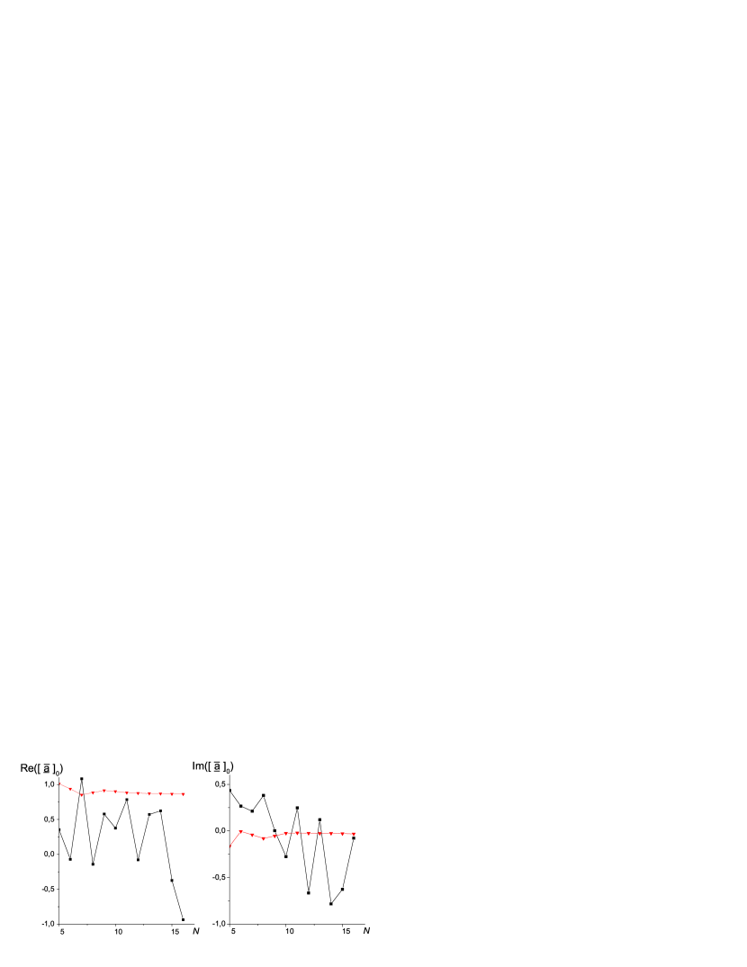
Figure 4: The convergence behavior of $\left[\overline{\underline{a}}\right]_{0}$ as the number $N$ of basis functions (31) for each of the coordinates $\xi_{1},\,\xi_{2},\,\xi_{3}$ is increased. The coefficient values obtained without and with smoothing factors are denoted by squares and triangles, respectively.

Table 1: Convergence of the first few “reduced” coefficients $\left[\underline{\overline{a}}\right]_{\mathfrak{N}}$. $N$ is the number of the basis functions (31) ($N=N_{1}=N_{2}=N_{3}$) in the expansion (32).

$N$	$n_{1}=n_{2}=n_{3}=0$	$n_{1}=1,\,n_{2}=n_{3}=0$	$n_{1}=n_{2}=0,\,n_{3}=1$
0	$1.00000000+i0.00000000$	$0.33332667-i1.33332667$	$-1.33333333+i0.33333333$
5	$1.00869682-i0.16338707$	$0.06484035-i1.03904748$	$-0.89298931+i0.33045941$
6	$0.93751779-i0.00481271$	$0.21244616-i1.16523626$	$-1.09329190+i0.31413236$
7	$0.85258743-i0.04143155$	$0.28687445-i1.10607051$	$-1.09100360+i0.21980636$
8	$0.88418841-i0.08046765$	$0.25361563-i1.06748525$	$-1.04328109+i0.23545010$
9	$0.91352864-i0.05297516$	$0.22333705-i1.09569062$	$-1.06280041+i0.27685677$
10	$0.90101510-i0.02409631$	$0.23719582-i1.12705918$	$-1.10091006+i0.27238506$
11	$0.88184853-i0.02083012$	$0.25897978-i1.13142201$	$-1.11043846+i0.25184571$
12	$0.87486976-i0.02519219$	$0.26812774-i1.12658516$	$-1.10795951+i0.24433839$
13	$0.87207818-i0.02578117$	$0.27172914-i1.12525415$	$-1.11016454+i0.24216317$
14	$0.86790716-i0.02592191$	$0.27617970-i1.12505442$	$-1.11300765+i0.23690466$
15	$0.86415304-i0.02795984$	$0.28050647-i1.12351749$	$-1.11247348+i0.23154456$
16	$0.86200713-i0.03060950$	$0.28381235-i1.12130593$	$-1.11061131+i0.22824086$

References

• (1) I. Bray and A. T. Steblovics, Phys. Rev. Lett., 70, 746 (1993).
• (2) I. Bray, D. V. Fursa, A. S. Kheifets, and A. T. Steblovics, J. Phys. B, 35, R117 (2002).
• (3) Z. Papp, Phys. Rev. C, 55, 1080 (1997).
• (4) Z. Papp, C-. Y. Hu , Z. T. Hlousek, B. Kónya, and S. L. Yakovlev, Phys. Rev. A, 63, 062721 (2001).
• (5) The J-Matrix Method: Developments and Applications, Ed. by A. D. Alhaidari, E. J. Heller, H. A. Yamani, and M. S. Abdelmonem (Springer Sci., Business Media, 2008).
• (6) S. A. Zaytsev, V. A. Knyr, Yu. V. Popov, A. Lahmam-Bennani, Phys. Rev. A, 76, 022718 (2007).
• (7) M. Silenou Mengoue, M. G. Kwato Njock, B. Piraux, Yu. V. Popov, and S. A. Zaytsev, Phys. Rev. A, 83, 052708 (2011).
• (8) A. L. Frapiccini, J. M. Randazzo, G. Gasaneo, and F. D. Colavecchia, J. Phys. B, 43, 101001 (2010).
• (9) A. S. Kadyrov, I. Bray, A. M. Mukhamedzhanov, and A. T. Steblovics, Phys. Rev. Lett., 101, 230405 (2008).
• (10) S. A. Zaytsev, J. Phys. A, 41 265204 (2008).
• (11) S. A. Zaytsev, J. Phys. A, 42 015202 (2009).
• (12) S. A. Zaytsev, J. Phys. A, 43 385208 (2010).
• (13) H. Klar, Z. Phys. D, 16, 231 (1990).
• (14) L. Rosenberg, Phys. Rev. D, 8, 1833 (1973).
• (15) Dz. Belkic, J. Phys. B, 11, 3529 (1978).
• (16) C. R. Garibotti, J. E. Miraglia, Phys. Rev. A, 21, 572 (1980).
• (17) M. Brauner, J. S. Briggs, H. Klar, J. Phys. B, 22, 2265 (1989).
• (18) S. Jones and D. H. Madison, Phys. Rev. Lett., 91, 073201 (2003).
• (19) L. U. Ancarani, T. Montagnese, and C. Dal Capello, Phys. Rev. A, 70, 012711 (2004).
• (20) O. Chuluunbaatar, H. Bachau, Yu. V. Popov, B. Piraux, K. Stefańska, Phys. Rev. A, 81, 063424 (2010).
• (21) P. A. Macri, J. E. Miraglia, C. R. Garibotti, F. D. Colavecchia and G. Gasaneo, Phys. Rev. A, 55, 3518 (1997).
• (22) P. C. Ojha, J. Math. Phys. 28, 392 (1987).
• (23) C. Canuto, A. Quarteroni, M. Y. Hussaini, T. A. Zang, Spectral Methods. Fundamentals in Single Domains (Springer-Verlag, Berlin, Heidelberg, 2006).
• (24) M. Stone, Mathematics for Physics I (Pimander-Casaubon, Alexandria, Florence, London, 2002).
• (25) J. Révai, M. Sotona, and J. Žofka, J. Phys. G, 11, 745 (1985).
• (26) B. Kónya, G. Lévai, and Z. Papp, Phys. Rev. C, 61 034302 (2000).
• (27) J. Berakdar, Phys. Rev. A, 53, 3214 (1996).
• (28) R. A. Swainson, G. W. Drake, J. Phys. A, 24 95 (1991).
• (29) M. Abramowitz and I. A. Stegun, Handbook of mathematical functions (New York: Dover), 1970.
• (30) L. D. Faddeev and S. P. Merkuriev, Quantum Scattering Theory for Several Particle Systems (Kluwer Academic Publishers, Dordrecht, 1993).
• (31) V. S. Buslaev, S. B. Levin, 2011, arXiv:1104.3358v1 [math-ph].
Refer to caption