Phase resolved spectroscopic study of the isolated neutron star RBS 1223 (1RXS J130848.6+212708)

Abstract

Aims. To constrain the mass-to-radius ratio of isolated neutron stars, spin-phase resolved X-ray spectroscopic analysis is performed.

Methods. The data from all observations of RBS 1223 (1RXS J130848.6+212708) conducted by XMM-Newton EPIC pn with the same instrumental setup in 2003-2007 were combined to form spin-phase resolved spectra. A number of complex models of neutron stars with strongly magnetized ($B_{\mathrm{pole}}\sim 10^{13}-10^{14}$ G) surface, with temperature and magnetic field distributions around magnetic poles, and partially ionized hydrogen thin atmosphere above it have been implemented into the X-ray spectral fitting package XSPEC for simultaneous fitting of phase-resolved spectra. A Markov-Chain-Monte-Carlo (MCMC) approach is also applied to verify results of fitting and estimating in multi parameter models.

Results. The spectra in different rotational phase intervals and light curves in different energy bands with high S/N ratio show a high complexity. The spectra can be parameterized with a Gaussian absorption line superimposed on a blackbody spectrum, while the light curves with double-humped shape show strong dependence of pulsed fraction upon the energy band (13% – 42%), which indicates that radiation emerges from at least two emitting areas.

Conclusions. A model with condensed iron surface and partially ionized hydrogen thin atmosphere above it allows us to fit simultaneously the observed general spectral shape and the broad absorption feature observed at 0.3 keV in different spin phases of RBS 1223. It allowed to constrain some physical properties of X-ray emitting areas, i.e. the temperatures ($T_{\mathrm{p1}}\sim 105$ eV, $T_{\mathrm{p2}}\sim 99$ eV), magnetic field strengths ($B_{\mathrm{p1}}\approx B_{\mathrm{p2}}\sim 8.6\times 10^{13}$ G) at the poles, and their distributions parameters ($a_{\mathrm{1}}\sim 0.61,a_{\mathrm{2}}\sim 0.29$, indicating an absence of strong toroidal magnetic field component). In addition, it puts some constraints on the geometry of the emerging X-ray emission and gravitational redshift ($z=0.16^{+0.03}_{-0.01}$) of RBS 1223.

1 Introduction

The study of thermally emitting, radio-quiet, nearby, isolated neutron stars (INSs) may have an important impact on our understanding of the physics of neutron stars. Observations and modeling of thermal emission from INSs can provide not only information on the physical properties such as the magnetic field, temperature, and chemical composition of the regions where this radiation is produced, but also information on the properties of matter at higher densities deeper inside the star.

In particular, measuring the gravitational redshift of an identified spectral feature in the spectrum of thermal radiation emitted from the INS surface/atmosphere may provide a useful constraint on theoretical models of equations of state for superdense matter. Independent of the estimate of the INS radius (e.g. Trümper et al. 2004) from the thermal spectrum of an INS, it may allow us to directly estimate the mass-to-radius ratio.

Much more information may be extracted by studying spin-phase resolved spectra with high signal to noise ratio and fitting them with model spectra of radiation emitted from highly magnetized INS surface layers.

RBS 1223 (1RXS J130848.6+212708) was originally discovered as a soft X-ray source during the ROSAT All-Sky Survey by Schwope et al. (1999). It shared common characteristics with other members of the small group (so far 7 discovered by ROSAT) of thermally emitting and radio-quiet, nearby INSs, traditionally dubbed XDINS (from “X-ray dim INS”) or Magnificent Seven (see, e.g., reviews by Haberl 2007; Mereghetti 2008; Turolla 2009, and references therein): soft spectra, well described by blackbody radiation with temperatures 60 – 120 eV, no other spectral features, no association with SNR, no radio emission, no X-ray pulsations, very high X-ray to optical flux ratio. A nature of these sources as old INS reheated by accretion from the interstellar medium or young cooling stars seemed possible. Meanwhile, intensive X-ray observations with mainly XMM-Newton and also with Chandra, as well as optical/UV observations of most probable counterparts, have revised this picture in parts and has provided intriguing physical insight.

X-ray pulsations have been found in six of these objects, with periods clustered at 3 – 11 sec, and period derivatives have been measured for five of them. In a classic $P-\dot{P}$ diagram the XDINSs are found intermediate between radio pulsars and magnetars (e.g., Mereghetti 2008). The inferred magnetic field strengths are above $10^{13}$ G.

Imaging CCD-spectroscopy with XMM-Newton has uncovered absorption features in at least three, likely in six stars. At current energy resolution ($\textrm{FWHM}\sim 50$ – 150 eV between $0.2$ – 2.0 keV) they can be, formally, well fitted as a Gaussian absorption lines, which are usually connected with ion cyclotron lines. Their interpretation is not unique, magnetically shifted atomic transitions or electron cyclotron resonances are debated. For some of the models, the inferred magnetic field strengths are again above $10^{13}$ G (Haberl 2007).

Among them, RBS 1223 is a special case, some sort of outlier, qualitatively different from the typical pattern observed in the sample of XDINSs. Namely, the rotational phase folded light curve has a double-humped shape, with largest pulsed fraction ($\sim$ 19% in 0.2-1.2 keV energy range, see further). Moreover, the separation of maxima by less than 180 degrees, significantly different count-rates of minima, and the variation of the blackbody apparent temperatures between 80 and 90 eV over the spin cycle are evidence for, at least, two emitting areas with some temperature distribution over neutron star surface (Schwope et al. 2005, 2007).

It is worth to note that the abovementioned observed absorption feature at $\sim$ 0.3 keV in the spectrum of RBS 1223 has the highest equivalent width ($\sim$ 0.2keV, Schwope et al. 2007) among all XDINSs. Moreover, spectral analysis of the average XMM-Newton spectrum of RBS 1223 (Schwope et al. 2007) based on the two first observations (see Table 1) showed the possible presence of a second feature in the X-ray spectrum. Its existence, however, is not uniquely proven because of some remaining calibration uncertainties and the not well-defined continuum at high energies because of the lack of photons (lower S/N ratio).

Meanwhile, new observational sets (see Table 1) are publicly available and a number of new detailed models of emergent spectra of highly magnetized INSs are developed and available (Ho et al. 2009; Suleimanov et al. 2010a).

Preliminary analysis of the phase averaged spectrum of RBS 1223 was performed by Pérez-Azorín et al. (2006b). They mentioned that there is a possibility of good fits with quadrupolar magnetic fields, although not excluding a condensed surface model with hydrogen atmosphere, including vacuum polarization effects (van Adelsberg & Lai 2006).

To explain unusual observed properties of RBS 1223 Suleimanov et al. (2010a, hereafter Paper I) studied various local models of the emitting surface of this INS. They considered three types of models: naked condensed surfaces, semi-infinite partially ionized hydrogen atmospheres with vacuum polarization and partial mode conversion taken into account (see details in Suleimanov et al. 2009) and such thin atmospheres above condensed iron surface. They also created a code for modeling integral phase resolved spectra and light curves of rotating neutron stars. This code takes into account general relativistic effects and allows one to consider various temperature and magnetic field distributions. Analytical approximations of the considered three types of local spectra were used for such modeling. It was qualitatively shown that only a thin model atmosphere above a condensed iron surface can explain the observed equivalent width of the absorption feature and the pulsed fraction.

In this paper we use the code developed in Paper I to perform a comprehensive study of co-added high-S/N and phase-resolved XMM-Newton EPIC pn spectrum of RBS 1223, despite a possible small variations of brightness shown by this INS (see Fig. 1).

Figure 1: Observed count rates of RBS1223 in the energy band 0.16 – 2.0 keV in different XMM-Newton EPIC pn observations.

2 Observations and data reduction

RBS 1223 has been observed many times by XMM-Newton (Table 1). Here we focus on the data collected with EPIC pn (den Herder et al. 2001) from the 12 publicly available observations, with same instrumental setup (Full Frame mode, Thin1 filter, positioned on axis), in total presenting about 175 ks of effective exposure time.

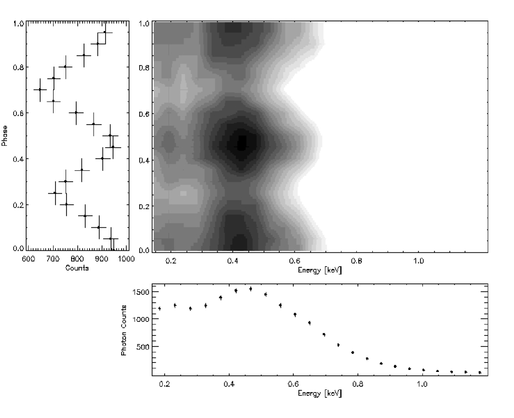
Figure 2: Energy-Phase image of RBS1223 combined from different observations. Rotational phase-folded light curve in the broad energy, 0.2-2.0 keV, band (left panel) and the phase averaged spectrum (bottom panel) are shown.

Table 1: XMM-Newton EPIC pn observations of RBS1223

Obs. ID	Obs. Date	Exposure	Effective exposure
	MJD	ksec	ksec
0157360101	52640.4271023	28.910	25.966
0163560101	53003.4674787	32.114	26.436
0305900201	53546.0889925	16.806	11.443
0305900301	53548.0919318	14.812	12.682
0305900401	53566.4161765	14.814	10.574
0305900601	53745.8803029	16.845	14.702
0402850301	53894.9783016	7.419	4.761
0402850401	53902.9489095	8.421	5.558
0402850501	53913.2292603	12.517	2.801
0402850701	53921.2857528	10.411	6.366
0402850901	54096.6780925	9.315	8.011
0402851001	54262.6501350	10.920	8.462

The data were reduced using standard threads from the XMM-Newton data analysis package SAS version 10.0.0. We reprocessed all publicly available data (see Table 1) with the standard metatask epchain. To determine good time intervals free of background flares, we applied filtering expression on the background light curves, performing visual inspection. This reduced the total exposure time by $\sim$ 30%. Solar barycenter corrected source and background photon events files and spectra were produced from the cleaned SINGLE events, using an extraction radius of 30$\arcsec$ in all pointed observations. We extracted also light curves of RBS 1223 and corresponding backgrounds from nearby, source free regions. We then used the SAS task epiclccorr to correct observed count rates for various sorts of detector inefficiencies (vignetting, bad pixels, dead time, effective areas, etc.) in different energy bands for each pointed observation (see Fig. 1).

For each registered photon the corresponding rotational phase was computed according to the phase coherent timing solution provided by Kaplan & van Kerkwijk (2005). We produced spin phase-folded light curves in different energy bands and spectra corresponding to different phase intervals for each pointed observation. Finally, the latter ones were co-added for the same intervals of phases to create the combined phase-resolved spectra of RBS 1223 (Fig. 2).

It should be noted that spectral responses and effective areas for those 12 different observations were almost undistinguishable.

3 Data analysis

First, we have fitted the phase-averaged, high signal-to-noise ratio spectral data, collected from different observations (Fig. 3 and Table 2), using a combination of an absorbed blackbody and a Gaussian absorption line multiplicative component model (in XSPEC phabs*bbodyrad*gabs).

Table 2: Fitting results by model phabs*gabs*bbodyrad ($\tau=0.612\pm 0.08,\sigma=0.155\pm 0.008,N_{H}=(1.8\pm 0.0035)\times 10^{18}cm^{-2}$) .

Phase interval	kT	Line center	Remarks
	(keV)	(keV)
0.20$-$0.35	0.084$\pm$0.001	0.25$\pm$0.01	First minimum
0.35$-$0.65	0.088$\pm$0.001	0.26$\pm$0.01	Secondary peak
0.65$-$0.80	0.083$\pm$0.001	0.24$\pm$0.01	Second minimum
0.0$-$0.2,0.8$-$1.0	0.088$\pm$0.001	0.29$\pm$0.01	Primary peak
0.00$-$1.0	0.086$\pm$0.001	0.27$\pm$0.01	Phase averaged

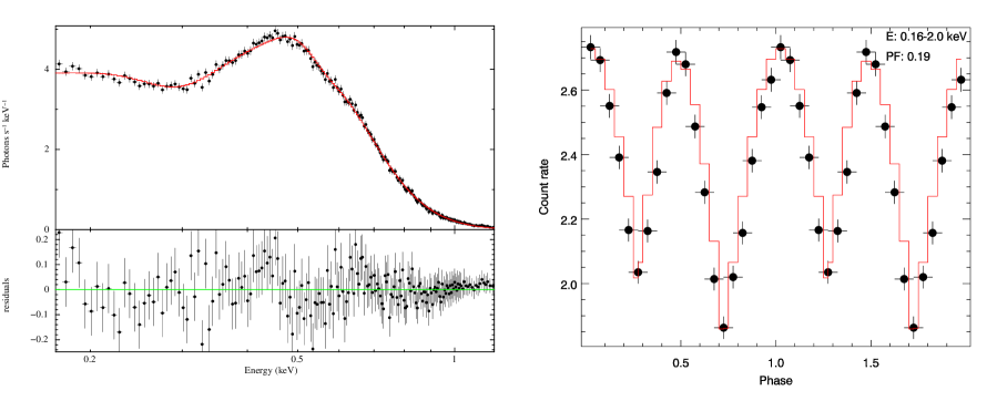
Figure 3: Phase-averaged X-ray spectrum (left panel) and phase-folded light curve (right panel) in the broad energy band of 0.16-2.0 keV of RBS 1223 combined from 12 pointed XMM-Newton EPIC pn observations.

In the spectral energy range of 0.16$-$2.0 keV we obtained a statistically acceptable fit with the reduced $\chi^{2}=1.1$.

We performed also a fit with the abovementioned spectral model for four phase intervals, including maxima and minima of the double-humped phase folded light curve, simultaneously. The fitted parameters are presented in Table 2. It shows a dependence of the blackbody apparent temperature and the Gaussian absorption feature center upon rotational phase. Next, we divided the broad energy band into four energy regions (0.16–0.5, 0.5–0.6, 0.6–0.7, and 0.7–2.0 keV) and constructed rotational phase folded light curves (Fig. 4). It is also noteworthy that the higher the considered spectral energy range, the larger the pulsed fraction. These spin phase-folded light curves may serve for rough estimates of the viewing geometry and physical characteristics of emitting areas of RBS 1223 (see below). In particular, the obtained parameters of the fits at different phases (Table 2) support a model with hot areas around the magnetic poles, because the energies of line centers and the blackbody temperatures are larger at the peaks.

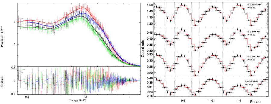
Figure 4: X-ray spectra including primary and secondary peaks, first and second minima, and phase-folded light curves in different energy bands of RBS 1223 combined from 12 pointed XMM-Newton EPIC pn observations. Fitted absorbed blackbody with gaussian absorption line models (phabs*bbodyrad*gabs XSPEC) to the spectra and two sinusoids to the phase-folded light curves are also shown (for details, see text and Table 2).

Dotted vertical lines are indicating phase intervals used for extraction and fitting of spectra shown in the left panel.

In view of this result, we implemented into the X-ray spectral fitting package XSPEC a number of new highly magnetized INS surface/atmosphere models developed in Paper I. They are based on various local models and compute rotational phase dependent integral emergent spectra of INS, using analytical approximations. The basic model includes temperature/magnetic field distributions over INS surface, viewing geometry and gravitational redshift. Three local radiating surface models are also considered, namely, a naked condensed iron surface and partially ionized hydrogen model atmospheres, semi-infinite or finite on top of the condensed surface. Here we have reproduced the essential part of the basic model (for details and further references, see Paper I).

To compute an integral spectrum, the model uses an analytical expression for the local spectra: a diluted blackbody spectrum for both semi-infinite and thin models of a magnetized atmosphere with one absorption feature:

$$I_{\mathrm{E}}(\alpha)=D\leavevmode\nobreak\ B_{\mathrm{E}}(T)\leavevmode\nobreak\ \phi(\alpha)\,\exp(-\tau),$$ (1)

where $\alpha$ is the angle between radiation propagation direction and the surface normal, and $\phi(\alpha)$ represents the considered angular distributions of the specific intensities for different cases of atmosphere models. We have represented $\phi(\alpha)$ by the following three models:

$$\phi(\alpha)=\left\{\begin{array}[]{ll}1,&\mathrm{\,a},\\ 0.4215+0.86775\cos\alpha,&\mathrm{\,b},\\ \left\{\begin{array}[]{l}\displaystyle\frac{1-0.2\cos^{2}\alpha_{\mathrm{c}}}{1-\cos^{2}\alpha_{\mathrm{c}}},\quad\textrm{if\leavevmode\nobreak\ \leavevmode\nobreak\ }\left\{\begin{array}[]{l}\cos\alpha\geq\cos\alpha_{\mathrm{c}}\\ \textrm{and\leavevmode\nobreak\ \leavevmode\nobreak\ }E_{\mathrm{c,i}}<E<4E_{\mathrm{C}},\end{array}\right.\\ 0.2,\quad\textrm{if}\leavevmode\nobreak\ \leavevmode\nobreak\ \leavevmode\nobreak\ \cos\alpha<\cos\alpha_{\mathrm{c}}\textrm{\leavevmode\nobreak\ \leavevmode\nobreak\ and\leavevmode\nobreak\ \leavevmode\nobreak\ }E_{\mathrm{c,i}}<E<4E_{\mathrm{C}},\\ 1\quad\textrm{for other\, energies}.\end{array}\right\}&\mathrm{\,c}.\\ \end{array}\right.$$

Here, the cases a, b, and c correspond to the models of isotropic emission, electron scattering directivity pattern, and a finite hydrogen atmosphere layer above a condensed iron surface, respectively; $\cos\alpha_{\mathrm{c}}=\left[\frac{1}{3}\left(E_{\mathrm{C_{\mathrm{1}}}}/E_{\mathrm{C}}-1\right)\right]^{2/3}$ is a parameter of angular distribution for the case of a thin atmosphere in the energy range $E_{\mathrm{ci}}<E<4E_{\mathrm{C}}$; $E_{\mathrm{c,i}}=\hbar\leavevmode\nobreak\ ZeB/m_{\mathrm{i}}c$ and $E_{\mathrm{c,e}}=\hbar eB/m_{\mathrm{e}}c$ are the ion and electron cyclotron energies, $E_{\mathrm{p,e}}=\hbar\sqrt{4\pi e^{2}n_{\mathrm{e}}/m_{\mathrm{e}}}$ is the electron plasma energy, $Z$ and $m_{\mathrm{i}}$ are the ion charge number and ion mass, $n_{\mathrm{e}}$ is the electron number density, $B$ the magnetic field strength,

$$E_{\mathrm{C}}=E_{\mathrm{c,i}}+E_{\mathrm{p,e}}^{2}/E_{\mathrm{c,e}},$$ (2)

and

$$E_{\mathrm{C_{1}}}=E_{\mathrm{C}}\leavevmode\nobreak\ (1+3(1-\cos\alpha)^{3/2}).$$ (3)

The optical depths $\tau=\tau^{0}\exp\left(-\frac{(E-E_{\mathrm{line}})^{2}}{2\sigma_{\mathrm{line}}^{2}}\right)$ and the widths $\sigma_{\mathrm{line}}$ of the absorption features are considered identical for all local spectra, but the center of the line depends on the local magnetic field strength. In the case of a semi-infinite atmosphere this absorption line represents the blend of the proton cyclotron line and nearby b-b atomic transitions in neutral hydrogen. The line center corresponds to the proton cyclotron energy $E_{\mathrm{c,H}}$. In the case a thin atmosphere the absorption feature was represented by a half of a Gaussian line. It means that $\tau^{0}=0$ at $E<E_{\mathrm{line}}$. This half of the Gaussian line represents a the complex absorption feature, which includes a broad absorption feature from the emitting condensed iron surface transmitted through a thin hydrogen atmosphere and the proton cyclotron line plus b-b atomic hydrogen transitions (see details in Paper I). The center of this line corresponds to the ion cyclotron $E_{\mathrm{c,i}}$ for completely ionized iron. In both cases, the absorption details are better represented by sums of two or even three Gaussian lines. But we have chosen to use only one (or half) Gaussian line to reduce the number of fitting parameters. The local spectra of the condensed iron surface is approximated by simple step functions (see Paper I). The dilution factor $D$ cannot be found from the fitting independently, and we take $D=1$ for all local spectra.

The blackbody temperature and the magnetic field distributions in the two emitting areas around the magnetic poles were presented analytically by Pérez-Azorín et al. (2006a):

$$T^{4}=T_{\mathrm{p1,2}}^{4}\frac{\cos^{2}\theta}{\cos^{2}\theta+a_{\mathrm{1,2}}\sin^{2}\theta}+T_{\mathrm{min}}^{4}$$ (4)

and

$$B=B_{\mathrm{p1,2}}\sqrt{\cos^{2}\theta+a_{1,2}\sin^{2}\theta},$$ (5)

where $T_{\mathrm{p1,2}}$ and $B_{\mathrm{p1,2}}$ are the temperatures and magnetic field strengths at the poles and $a_{\mathrm{1,2}}$ their distribution parameters and $T_{\mathrm{min}}$ is the minimum temperature reached on the surface of the star (we chose $\approx 0.3T_{\mathrm{p}}$, like in Pérez-Azorín et al. 2006a). Here $\theta$ is the magnetic colatitude.

The parameters $a_{\mathrm{1,2}}$ are approximately equal to the squared ratio of the magnetic field strength at the equator to the field strength at the pole, $a_{\mathrm{1,2}}\approx(B_{\mathrm{eq}}/B_{\mathrm{p1,2}})^{2}$. Using these parameters we can describe various temperature distributions, from strongly peaked ($a\gg 1$) to the classical dipolar ($a=1/4$) and homogeneous ($a=0$) ones.

Finally, the total observed flux at distance $d$ from the INS is summed over the visible surface. A local spectrum at photon energy $E$ from the unit surface is computed taking into account viewing geometry, gravitational redshift, and light bending effects (e.g., Poutanen & Gierliński 2003):

$$f_{\mathrm{E}}\,d\,\varphi\,d\gamma=C_{\mathrm{norm}}\,(1+z)^{-3}\,I_{\mathrm{E^{\prime}}}(\alpha)\,\cos\alpha\,\sin\gamma\,d\,\varphi\,d\gamma,$$ (6)

where $C_{\mathrm{norm}}=R^{2}/d^{2}$ is a normalization constant and $\gamma$ is the angle between the radius vector at a given point and the rotation axis. The observed and emitted photon energies are related as $E=\leavevmode\nobreak\ E^{\prime}(1+z)$, where $z$ is gravitational redshift. The angle $\alpha$ between the emitted photon and normal to the surface in the local reference frame depends on $z$, the local surface position (on azimuthal and colatitude angles $\varphi$ and $\gamma$), and the angle between rotation axis and line of sight $i$, and is computed using the approximation of Beloborodov (2002). The summation is performed separately for both regions around magnetic poles, because we allow the poles to be not precisely antipodal (one of them can be shifted by angle $\kappa$ relative to the symmetric antipodal position). Therefore the poles may have different angles between rotation and magnetic axes $\theta_{\mathrm{B1,2}}$.

As shown in Paper I, a model with a thin hydrogen atmosphere above the condensed iron surface with a smooth temperature distribution over the neutron star surface may describe very well the observed physical properties of RBS 1223.

This basic model has a number of input parameters depending on the inner atmosphere boundary condition of an INS (condensed iron surface or blackbody, temperature and magnetic field distributions over surface, viewing geometry and gravitational redshift) and angular distribution of the emergent radiation (isotropic or peaked by a thin atmosphere above a condensed surface).

Combined spectra of RBS 1223 in 20 phase bins (Fig. 2) were considered as different data sets during simultaneous fitting with the absorbed abovementioned model. All input parameters were free and linked between those data groups.

Given the large number of the free parameters in the model we performed a preliminary analysis in order to get rough estimates of (or constraints on) some of them. From the observed double-humped light curve shape in different energy bands (see Fig. 4), it has been already clear that two emitting areas have different spectral and geometrical characteristics (e.g., the relatively cooler one has a larger size). Moreover, from the peak-to-peak separation in this double-humped light curve we locate the cooler one at an offset angle of $\kappa$ with respect to the magnetic axis and azimuth (Schwope et al. 2005).

First we performed formal spectral fitting with the simplest model, i.e. absorbed blackbody with multiplicative gaussian absorption line including phases of maxima (see Table 2) in the light curve (Figs. 3 and 4). It is clear, that at these phases X-ray emission is mostly dominated by emitting areas at the magnetic poles, where temperatures also have maxima (see formula of temperature and magnetic field dependence upon polar angle, Pérez-Azorín et al. 2006a and Paper I). Secondly, some constraints on magnetic field strengths at the poles may be used on the base of period and its derivative values assuming magnetic dipole breaking as a main mechanism of the spin down of RBS 1223.

Having these two general constraints on temperatures and magnetic field strengths at the poles we simulated a large number of photon spectra (absorbed blackbody with gaussian absorption line and different models considered in the Paper I) folded with the response of XMM-Newton EPIC pn camera, taking into account also the interstellar absorption (for parameters see Table 2, and using a characteristic magnetic field strength of B$\sim$ 3.4$\times$10¹³ Gauss).

The predicted phase-folded light curves in four spectral ranges: 0.16-0.5 keV, 0.5-0.6 keV, 0.6-0.7 keV, 0.7-2.0 keV and with free parameters of viewing geometry and gravitational redshift, normalized to the maximum of the brightness, we cross-correlated with observed ones (Fig. 4). We infer some constraints on the parameters from the unimodal distributions of them when cross-correlation coefficients were exceeding 0.9 in the mentioned four energy bands simultaneously and used them as initial input value and as lower and upper bounds for fitting purposes. For example, gravitational redshift cannot exceed 0.3 (it is not possible to obtain the observed PF at larger $z$ due to strong light bending) or the antipodal shift angle must be less than $25^{\circ}$ (due to the observed phase separation between the two peaks in the light curve). It is also evident that the sum of the inclination angle of the line of sight and magnetic poles relative to the rotational axis are already constrained by the light curve class (see, Poutanen & Beloborodov 2006, class III) and have the maximum effect (e.g., provide the maximum PF) when both are equal to $90^{\circ}$. It should be noted that these angles do not have a large influence on the fitting, and the only important issue is a range of values when two maxima are observed.

Having abovementioned crude constraints and input values of free parameters we performed fitting with the models implemented in XSPEC package of combined spectra of RBS 1223 in 20 phase bins (Fig. 2) simultaneously, i.e. each of those phase resolved spectrum considered as different data sets with the linked parameters to the others, and the only differences were phase ranges, which were fixed for an individual phase resolved spectrum.

The fitting was successful, with C-statistic value 2937 with 2159 degrees of freedom. These parameters are presented in Table 3.

Table 3: Simultaneous fitting results of combined, phase resolved X-ray spectra of RBS1223 with different spectral models

Fitted	Spectral Model
Parameter	Iron condensed surface	Blackbody
	partially ionized H atmosphere	electron scattering
$T_{\mathrm{p1}}\leavevmode\nobreak\ \mathrm{[eV]}$	$\mathrm{105.0_{-4.0}^{+2.0}}$	$109\pm 4.0$
$T_{\mathrm{p2}}\leavevmode\nobreak\ \mathrm{[eV]}$	$99.0\pm 3.0$	$106\pm 3.0$
$B_{\mathrm{p1}}\times 10^{14}\leavevmode\nobreak\ \mathrm{[G]}$	$0.86\pm 0.02$	$0.65\pm 0.03$
$B_{\mathrm{p2}}\times 10^{14}\leavevmode\nobreak\ \mathrm{[G]}$	$0.86\pm 0.02$	$0.58\pm 0.02$
$a_{\mathrm{p1}}$	$0.61\pm 0.11$	0.25
$a_{\mathrm{p2}}$	$0.29\pm 0.05$	0.25
$\tau^{0}$	$\mathrm{2.76_{-0.02}^{+0.10}}$	$1.90\pm 0.06$
$\sigma\leavevmode\nobreak\ \mathrm{[eV]}$	$\mathrm{225.8_{-1.8}^{+5.6}}$	$168.0\pm 6.0$
$z$	$0.15\pm 0.02$	$0.17\pm 0.03$
$\kappa[{\degr}]$	$4.2\pm 0.6$	$4.0\pm 0.4$
${\it i[{\degr}]}$	$48.9\pm 0.5$	$45.6\pm 0.5$
$\theta[{\degr}]$	$90.0\pm 0.5$	$90.0\pm 0.5$

In order to assess a degree of uniqueness and to estimate confidence intervals of the determined parameters, we have additionally performed Markov Chain Monte Carlo (MCMC) fitting as implemented in XSPEC. In Fig. 5 we present probability density distributions of some of them. Note, independent initial input values of parameters of MCMC approach converged to the same values, in 6 different chains.

Figure 5: Probability density distributions of parameters (temperatures, magnetic field strengths at the poles, antipodal shift angle and gravitational redshift) by MCMC fitting with the model of a neutron star with condensed surface and partially ionized hydrogen layer above it. The most probable parameter value is indicated by the solid vertical line. Dashed vertical lines indicate the highest probability interval ($68\%$, for details see text).

4 Discussion

The combined phase-resolved spectra of RBS 1223 can be simultaneously fitted by emergent radiation of a spectral model of an iron condensed surface with a partially ionized hydrogen atmosphere above it. Formally they can be fitted also by a blackbody spectrum with proton-cyclotron absorption gaussian line and a peaked (typical for an electron scattering atmosphere) angular distribution of the emergent radiation. In both cases two emitting areas with slightly different characteristics are required (see Table 3).

It is worth to note, that the resulting fit parameters are very similar for different spectral models (see Table 3), which is also confirmed by an MCMC approach with different input parameters.

However, we believe that the emission properties due the condensed surface model with a partially ionized, optically thin hydrogen layer above it, including vacuum polarization effects, is more physically motivated. Moreover, semi-infinite atmospheres have rather fan-beamed emergent radiation (see Paper I and references within) and it seems impossible to combine a proton cyclotron line with a pencil-beamed emergent radiation.

We calculated a set of thin highly magnetized partially ionized hydrogen atmospheres above a condensed iron surface with magnetic field strength $B=8\times 10^{13}$ G, which is close to the value estimated from observations. The observed blackbody temperature of the spectra is reproduced at effective temperatures $T_{\mathrm{eff}}\approx 7\times 10^{5}$ K. Examples of the computed emergent spectra with parameters $B=8\times 10^{13}$ G, $T_{\mathrm{eff}}=7\times 10^{5}$ K and various atmosphere column densities $\Sigma$ are shown in Fig. 6. The emergent diluted blackbody spectrum with $T=0.1$ keV and the absorption Gaussian line parameters, presented in Table 3 ($\tau^{0}=2.8,\sigma_{\mathrm{line}}=0.226$ keV, $E_{\mathrm{line}}=0.24$ keV) and $D=0.34$  are also shown. Unfortunately, from these models we cannot evaluate the actual atmosphere thickness (the surface density), but we can obtain the dilution factor $D$, which is important to correct the distance estimation.

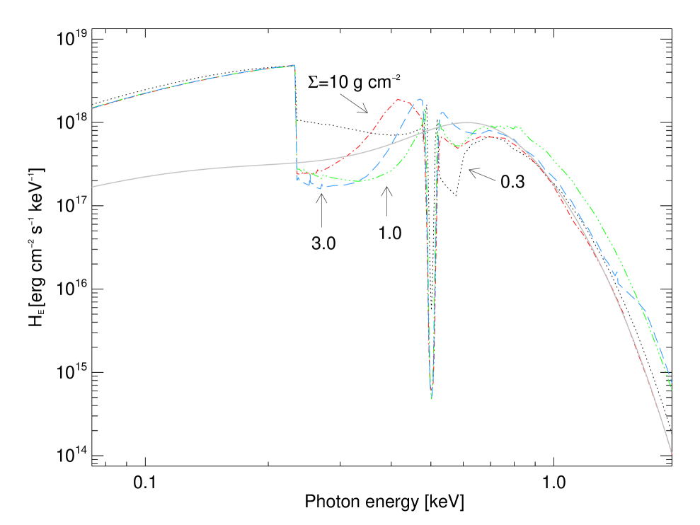
Figure 6: Emergent spectra of the fitted model of a magnetized atmosphere with a condensed iron surface and a partially ionized hydrogen layer above it (see Table 3). Different lines are corresponding different atmospheric surface densities. For comparison purposes a blackbody spectrum with gaussian absorption line is also shown in gray (see text).

Emission spectra based on realistic temperature and magnetic field distributions with strongly magnetized hydrogen atmospheres (or other light elements) are formally still an alternative, but it is unphysical because of the absorption line added by hand.

A purely proton-cyclotron absorption line scenario can be excluded owing to the equivalent width of the observed absorption spectral feature in the X-ray spectrum of RBS 1223. Magnetized semi-infinite atmospheres predict too low an equivalent width of the proton cyclotron line in comparison with the observed one.

Figure 7: Mass-radius relations for several equations of state (thin solid curves, Haensel et al. 2007), and a strange star (dashed). Thin dash-doted: curves of constant apparent radius $R_{\infty}=R/\sqrt{1-2GM/Rc^{2}}=$ 9,13 and 17 km (Trümper 2005).

This result of the fitting (with the condensed surface model with partially ionized, optically thin hydrogen atmosphere above it, including vacuum polarization effects) suggests a true radius of RBS 1223 of $16\pm 1\mathrm{km}$ for a standard neutron star of 1.4 solar mass, considerably larger than the canonical radius of 10 km; it is only marginally compatible with the range from $\approx 10$ km to $\approx 14$ km, allowed by modern theoretical equations of state of superdense matter (Haensel et al. 2007; Hebeler et al. 2010, and references therein), and indicates a very stiff equation of state of RBS 1223 (Fig. 7; Ho et al. 2007; Heinke et al. 2006; Suleimanov & Poutanen 2006; Suleimanov et al. 2010b, for similar results, see also).

With these estimates of the radius and normalization constant of the fit ($R/d\approx 0.0247$ km pc^-1), we obtained for the assessment of the distance of RBS 1223 $\sqrt{D}\,650_{-50}^{+25}\textrm{\leavevmode\nobreak\ pc}=\sqrt{D/0.34}\,380_{-30}^{+15}$ pc (see also Schwope et al. 2005).

5 Conclusions

The observed phase resolved spectra of the INS RBS 1223 are satisfactorily fitted with two slightly different physical and geometrical characteristics of emitting areas, by the model of a condensed iron surface, with partially ionized, optically thin hydrogen atmosphere above it, including vacuum polarization effects, as orthogonal rotator. The fit also suggests the absence of a strong toroidal magnetic field component. Moreover, the determined mass-radius ratio ($(M/M_{\sun})/(R/\mathrm{km})=0.087\pm 0.004$) suggests a very stiff equation of state of RBS 1223.

These results on RBS 1223 are promising, since we could find good simultaneous fits to the rotational phase-resolved spectra of RBS 1223 using analytic approximations for the abovementioned model implementation.

More work for detailed spectral model computation will be certainly worth to do in the near future and application to the phase-resolved spectra of other INSs. In particular, for RX J1856.5$-$3754 and RX J0720.4$-$3125, including high resolution spectra observed by XMM-Newton and Chandra with possibly other absorption features (Hambaryan et al. 2009; Potekhin 2010).