Discussion of “Estimating Random Effects via Adjustment for Density Maximization” by C. Morris and R. Tang

10.1214/10-STS349

Discussion of Estimating Random Effects via Adjustment for Density Maximization by C. Morris and R. Tang

and

We congratulate Morris and Tang for an interesting addition to empirical Bayes methods, and for tackling a difficult and nagging problem in variance estimation. The ADM adjustment appears to bring on interesting properties, not just in variance estimation but also in estimation of the means. In this discussion we want to focus on the latter topic, and see how the ADM-derived estimators of a normal mean perform in a decision-theoretic way. To facilitate this we will stay with the simple model

$$y_{i}|\theta_{i}\sim N(\theta_{i},V),\quad\theta_{i}\sim N(0,A).$$ (1)

1 The James–Stein Estimator as Generalized Bayes (Not!)

We first address the comment of Morris and Tang in Section 2.5, that the prior $A\sim\operatorname{Unif}(0,\infty)$ is strongly suggested because the James–Stein estimator is the posterior mean if we take $A\sim\operatorname{Unif}(-V,\infty)$. Professor Morris has noted this before, and in the interest of understanding, we want to show this calculation and comment on its relevance.

Writing $\mathbf{y}=(y_{1},\ldots,y_{k})$ and $\bolds{\theta}=(\theta_{1},\ldots,\theta_{k})$, the posterior expected loss from model (1), with the $A\sim\operatorname{Unif}(-V,\infty)$ prior, is

$$\int_{-V}^{\infty}\int_{\Re^{p}}|\bolds{\theta}-\delta(\mathbf{y})|^{2}$$

(2)

$$\hphantom{\int_{-V}^{\infty}\int_{\Re^{p}}}{}\cdot\frac{e^{-|\mathbf{y}-\theta|^{2}/(2V)}}{(2\pi V)^{k/2}}\frac{e^{-|\theta|^{2}/(2A)}}{(2\pi A)^{k/2}}d\bolds{\theta}\,dA,$$

and factoring the exponent in (1) and writing $B=V/(V+A)$ shows that

$$\bolds{\theta}|\mathbf{y},A \sim N\bigl{(}(1-B)\mathbf{y},V(1-B)\bigr{)},$$

$$A|\mathbf{y} \sim \biggl{(}\frac{1}{V+A}\biggr{)}^{k/2}e^{-({1}/{(2(V+A))})|\mathbf{y}|^{2}}.$$

The Bayes rules is the posterior mean, which we can calculate as

$$\mathrm{E}(\bolds{\theta}|\mathbf{y}) = \mathrm{E}[\mathrm{E}(\bolds{\theta}|\mathbf{y},A)]$$

$$= \mathrm{E}[(1-B)\mathbf{y}|\mathbf{y}]=[1-\mathrm{E}(B|\mathbf{y})]\mathbf{y}.$$

We now, very carefully, calculate $\mathrm{E}(B|\mathbf{y})$, yielding

$$\mathrm{E}(B|\mathbf{y}) \propto \int_{-V}^{\infty}\biggl{(}\frac{V}{V+A}\biggr{)}\biggl{(}\frac{1}{V+A}\biggr{)}^{k/2}$$

$$\hphantom{\int_{-V}^{\infty}}{}\cdot e^{-(1/{(2(V+A))})|\mathbf{y}|^{2}}\,dA$$

$$= V\int_{1/V}^{\infty}t^{k/2-1}e^{-t|\mathbf{y}|^{2}/2}\,dt$$

$${}+V\int_{0}^{1/V}t^{k/2-1}e^{-t|\mathbf{y}|^{2}/2}\,dt,$$

where we make the transformation $t=1/(V+A)$, with the first integral coming from $A\in(-V,0)$. Noting that the integrand is the kernel of a chi-squared density, we finally have

$$\qquad\mathrm{E}(B|\mathbf{y}) \propto \frac{V\Gamma(k/2)2^{k/2}}{(|\mathbf{y}|^{2})^{k/2}}[P(\chi^{2}_{k}\geq|\mathbf{y}|^{2}/V)$$

$$\hphantom{\frac{V\Gamma(k/2)2^{k/2}}{(|\mathbf{y}|^{2})^{k/2}}[}{}+P(\chi^{2}_{k}\leq|\mathbf{y}|^{2}/V)],$$

where $\chi^{2}_{k}$ is a chi-squared random variable with $k$ degrees of freedom. Since the chi-squared probabilities sum to 1, normalizing this expectation (dividing by $\frac{\Gamma(k/2-1)2^{k/2-1}}{(|\mathbf{y}|^{2})^{k/2-1}}$) results in $\mathrm{E}(B|\mathbf{y})=V(k-2)/|\mathbf{y}|^{2}$, yielding the James–Stein estimator. There are a number of things to note: [0.]

If this were a valid calculation, it would contradict such important papers as Brown (1971) and Strawderman and Cohen (1971), which providedcomplete characterizations of admissible generalized Bayes estimators.

In fact, Strawderman and Cohen [(1971), Section 4.5], explicitly tell us that the James–Stein estimator cannot be generalized Bayes.

In fact, the calculation leading to $\mathrm{E}(B|\mathbf{y})=V(k-2)/|\mathbf{y}|^{2}$ is invalid. To see this note that, starting from (1), with $A\sim U(-V,\infty)$, the prior on $\theta$ is

$$\int_{-V}^{\infty}\frac{e^{-|\theta|^{2}/(2A)}}{(2\pi A)^{k/2}}\,dA,$$

and, even if we take $k$ to be even to avoid complex integration, it is straightforward to verify that the integral over $(-V,0)$ is infinite.

What does this tell us about the James–Stein estimator? The “bad” part of the integral, which leads to the piece in (1) corresponding to $P(\chi^{2}_{k}\geq|\mathbf{y}|^{2}/V)$, is to be avoided. We can informally interpret this as pointing to the region where $|\mathbf{y}|^{2}/V$ is small, resulting in shrinkage factors that could be greater than 1 (in absolute value), and result in the James–Stein estimator both changing the sign and expanding $\mathbf{y}$. When we lop off this part, we are led to estimators such as the positive-part James–Stein estimator, or admissible estimators, like those based on (32) in Morris and Tang.

2 Minimaxity of ADM

The lesson from the previous section is to avoid estimators that do not control the shrinker to be between $0$ and $1$. So we turn to ADM and ask if it can do this. We find, interestingly, that the ADM approach will, almost automatically, give us a minimax estimator and, moreover, it controls the shrinker.

Typically, minimax estimators have been constructed using empirical Bayes arguments and a bit of customizing, or using formal Bayes derivations with priors like $A\sim\operatorname{Unif}(0,\infty)$. The derivation of Morris and Tang in Section 2.7 is a straightforward differentiation, and we can apply the following theorem. [This is Theorem 5.5, Chapter 5, Lehmann and Casella (1998), and can be traced back to Baranchik (1970).]

Theorem 1

Under model (1), the estimator

$$\delta(\mathbf{y})=\biggl{(}1-\frac{Vg(|\mathbf{y}|)}{|\mathbf{y}|^{2}}\biggr{)}\mathbf{y}$$

is minimax under the loss $|\bolds{\theta}-\delta(\mathbf{y})|^{2}$ if [0.]

the function $g(|\mathbf{y}|)$ is nondecreasing,

$0\leq g(|\mathbf{y}|)\leq 2(k-2)$.

In the notation of Morris and Tang, we are considering the case $r=0$, and writing $T=|\mathbf{y}|^{2}/(2V)$, the ADM shrinkage factor is

$$\quad\hat{B}=\frac{1}{T}\biggl{[}\frac{2(m-c+1)T}{T+m+1+\sqrt{(T-m-1)^{2}+4cT}}\biggr{]}.$$ (4)

Morris and Tang note that $\hat{B}$ is monotone decreasing in $T$, but for minimaxity we need the function in square brackets, which corresponds to $g(\cdot)$ of the theorem, to be nondecreasing. black As $T\rightarrow\infty$, the function converges to $m-c+1$. If this is the maximum, and is less than $2(k-2)$, then the estimator will be minimax. In fact, it is straightforward (but tedious) to show that the derivative of the function in square brackets is always nonnegative, so the function is nondecreasing and the estimator is minimax. For $c=1$ the bound can be satisfied by taking $m=(k-2)/2$, for $k\geq 3$.

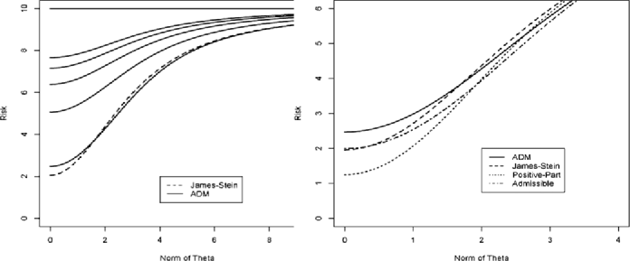
Figure 1: For dimension $k=10$, the left panel shows the risk of the James–Stein estimator (dashed line) and five ADM estimators (solid lines), for $m=(k-2)/2,(k-2)/4,(k-2)/6,(k-2)/8,(k-2)/10$. The risk function increases uniformly as the denominator increases, so $m^{\ast}=(k-2)/2$ gives the smallest risk. The right panel shows the risk of the ADM estimator with $m^{\ast}=(k-2)/2$ (solid), the James–Stein estimator (dashed), the positive-part estimator (dotted), and the admissible estimator with $B$ of (32) (dash-dot).

Unfortunately, this is as far as we can go. The estimator based on (4), which is reminiscent of a ridge regression estimator, cannot be admissible. Again we can trace this back to Strawderman and Cohen (1971), and also Berger and Srinivasan (1978). The problem is that (being a bit informal here) admissible estimators must be analytic in the complex plane which is not the case with those based on (4).

Lastly, we wanted to see the risk performance of ADM. Morris and Tang set $m=(k-2)/2$, but there is actually a range of values of $m$ for which the estimator is minimax. To clarify, denote $(k-2)/2=m^{\ast}$, the Morris and Tang choice, and consider the $m$ in (4) to be a variable. Then, for $c=1$ the estimator is minimax for all $m\leq 2(k-2)$. In Figure 1 we see, in the left panel, the risk of five ADM estimators, along with the risk of the James–Stein estimator for comparison. There we see that the choice of $m$ completely orders the ADM risk, with $m^{\ast}=(k-2)/2$ being the best choice, resulting in an estimator with risk similar to that of James–Stein. In the right panel we compare the ADM estimator, with $m^{\ast}=(k-2)/2$, to the James–Stein estimator, its positive-part version, and the admissible estimator with $B$ given in (32). There we see that ADM compares favorably with the James–Stein estimator, is uniformly dominated in risk by the admissible estimator, but not by the positive-part estimator, whose risk crosses that of ADM for large $|\theta|$.

3 Is ADM Automatic?

The automatic appearance of the ADM minimax estimator gives support to the claim of Morris and Tang that “ADM maintains the spirit of MLE while making small sample improvements.” In fact, examination of the ADM shrinker $B$, and its risk functions, shows that “automatic” ADM produces an estimator that does not shrink as strongly as either the admissible estimator or the positive-part and, hence, can have smaller risk for larger values of the norm of $\theta$. It is not clear to us that such small sample properties as minimaxity will continue to hold for other models, for example for the estimation of a Poisson mean, where many similar minimaxity results hold. However, the results of Morris and Tang are encouraging and certainly deserve further investigation.

References

- Baranchik (1970) {barticle}[mr] \bauthor\bsnmBaranchik, \bfnmA. J.\binitsA. J. (\byear1970). \btitleA family of minimax estimators of the mean of a multivariate normal distribution. \bjournalAnn. Math. Statist. \bvolume41 \bpages642–645. \bidissn=0003-4851, mr=0253461 \endbibitem
- Berger and Srinivasan (1978) {barticle}[mr] \bauthor\bsnmBerger, \bfnmJames O.\binitsJ. O. and \bauthor\bsnmSrinivasan, \bfnmC.\binitsC. (\byear1978). \btitleGeneralized Bayes estimators in multivariate problems. \bjournalAnn. Statist. \bvolume6 \bpages783–801. \bidissn=0090-5364, mr=0478426 \endbibitem
- Brown (1971) {barticle}[mr] \bauthor\bsnmBrown, \bfnmL. D.\binitsL. D. (\byear1971). \btitleAdmissible estimators, recurrent diffusions, and insoluble boundary value problems. \bjournalAnn. Math. Statist. \bvolume42 \bpages855–903. \bidissn=0003-4851, mr=0286209 \endbibitem
- Lehmann and Casella (1998) {bbook}[mr] \bauthor\bsnmLehmann, \bfnmE. L.\binitsE. L. and \bauthor\bsnmCasella, \bfnmGeorge\binitsG. (\byear1998). \btitleTheory of Point Estimation, \bedition2nd ed. \bpublisherSpringer, \baddressNew York. \bidmr=1639875 \endbibitem
- Strawderman and Cohen (1971) {barticle}[mr] \bauthor\bsnmStrawderman, \bfnmWilliam E.\binitsW. E. and \bauthor\bsnmCohen, \bfnmArthur\binitsA. (\byear1971). \btitleAdmissibility of estimators of the mean vector of a multivariate normal distribution with quadratic loss. \bjournalAnn. Math. Statist. \bvolume42 \bpages270–296. \bidissn=0003-4851, mr=0281293 \endbibitem