Discussion of “Estimating Random Effects via Adjustment for Density Maximization” by C. Morris and R. Tang

10.1214/10-STS349

Discussion of Estimating Random Effects via Adjustment for Density Maximization by C. Morris and R. Tang

and

We thoroughly enjoyed reading this excellent authoritative paper full of interesting ideas, whichshould be useful in both Bayesian and non-Bayesian inferences. We first discuss the accuracy of the ADM approximation to a Bayesian solution in a real-life application and then discuss how some of the ideas presented in the paper could be useful in a non-Bayesian setting.

How Does the ADM Work in a Real Application?

Although the main objective of this paper is to make inferences on the high-dimensional parameters or the random effects $\theta_{i}$, the authors note that the success of the Bayesian method lies on the accurate estimation of the shrinkage parameters $B_{i}$ since they appear linearly in the expressions for the posterior mean and posterior variance of $\theta_{i}$ when the hyperparameters are known. Thus, we assess the accuracy of the ADM approximation, given in Section 2.8, relative to the standard first-order Laplace approximation, in approximating the posterior distribution of the shrinkage factors for the hierarchical model (1)–(2). This model, commonly referred to as the Fay–Herriot model in the small area literature, was used by Fay and Herriot (1979) in order to combine survey data and different administrative records in producing empirical Bayes estimates of per-capita income of small places. Since then the Fay–Herriot model and its variants have been used in various federal programs such as the Small Area Income and Poverty Estimates (SAIPE) and the Small Area Health Insurance estimates (SAHIE) programs of the U.S. Census Bureau.

For purposes of evaluation, we consider the problem of estimating the proportion of 5- to 17-year-old (related) children in poverty for the fifty states and the District of Columbia using the same data set considered by Bell (1999). We choose two years (1993 and 1997) of state-level data from the SAIPE program. In 1993, the REML estimate of $A$ is positive while in year 1997 it is zero. The choice of these two years will thus give us an opportunity to assess the accuracy of the ADM approximations in two different scenarios.

We assume the standard SAIPE state-level model in which survey-weighted estimates of the proportions follow the two-level model given by (1)–(2). The survey-weighted proportions are obtained using the Current Population Survey (CPS) data with their variances $V_{i}$ estimated by a Generalized Variance Function (GVF) method, following Otto and Bell (1995), but assumed to be known throughout the estimation procedure. We use the same state-level auxiliary variables $x_{i}$ (a vector of length 5, i.e., $r=5$), obtained from Internal Revenue Service (IRS) data, food stamp data and Census data that the SAIPE program used for the problem. We assume the uniform prior on $\bolds{\beta}$ and superharmonic (uniform) prior on $A$, as used in the Morris–Tang paper.

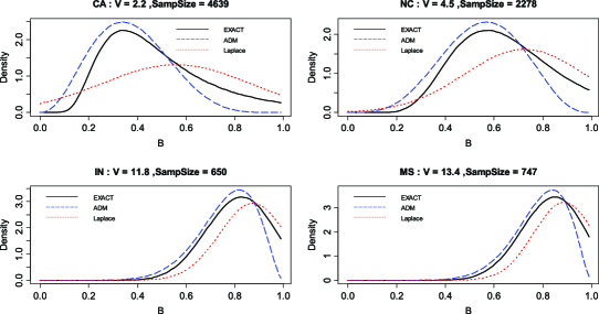
Figure 1: Plot of exact posterior density of $B_{i}$ along with approximate densities using SAIPE 1993 state-level data. The four states in the plot are taken from Bell (1999).

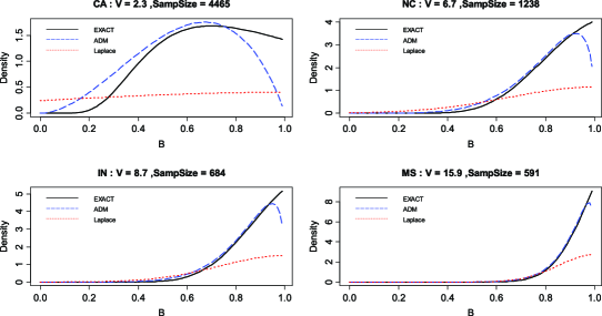
Figure 2: Plot of exact posterior densities of the shrinkage factors $B_{i}$ along with approximate densities using SAIPE 1997 data; the four states in the plot are taken from Bell (1999).

For the presentation of our results, we consider a selection of four states—California (CA), North Carolina (NC), Indiana (IN) and Mississippi (MS)—considered by Bell (1999). This selection represents both small (i.e., large $V_{i}$) and large (i.e., small $V_{i}$) states and thus should give us a fairly general idea of the degree of accuracy of the Laplace and ADM approximations with varying $V_{i}$ when compared to the exact posterior distributions of the shrinkage factors obtained by one-dimensional numerical integration.

First, consider the year 1993 when the REML estimate of $A$ is positive (1.7). The exact posterior distributions of the shrinkage factors, ADM approximations and the first-order Laplace approximations (Kass and Steffey, 1989) are plotted in Figure 1. The solid curves in Figures 1 and 2 are the exact posterior distributions of $B_{i}$, which are obtained from the posterior of $A$, under the prior, after multiplying bythe Jacobian and normalizing through numerical one-dimensional integration. The dotted lines are first-order Laplace approximations to the posterior distributions of $B_{i}$, which are simply normal distributions with means identical to $B_{i}$ with $A$ replaced by its posterior mode and variance expressions given in Kass and Steffy (1989). Thus, the posterior means and variances of $B_{i}$ are essentially approximated by the first-order Laplace method. From the plot it is clear that the ADM approximation is far better than the first-order Laplace approximation when we compare them with the exact posterior distribution of $B_{i}$.

Table 1 displays the exact posterior means and variances as well as their approximations for these states. In general, the ADM approximation appears to be fairly accurate with an indication of under-approximation of the posterior mean, especially for states with small $V_{i}$ (CA, NC). On the other hand, the first-order Laplace approximation generally overestimates the exact posterior means, sometimes by a large margin, and approximates shrinkage factors for all the states in the year 1997 by 1. Turning to the posterior variances, we observe that the first-order Laplace method generally over-approximates the exact posterior variances, sometimes by a large margin, especially for the year 1997. The poor performance of the Laplace method, for the SAIPE 1997 data, can be attributed to the fact that the use of uniform prior on $A$ yields a posterior mode that lies on the boundary. The ADM approximation appears to perform well for both the years, especially for 1997 when the Laplace method breaks down. For the year 1993, the ADM method appears to slightly under-approximate the exact posterior variances, especially for the states with small $V_{i}$. Overall, it appears that the accuracy of the ADM approximation depends somewhat on the states—the larger the $V_{i}$ the better the approximation accuracy.

Table 1: Comparison of posterior moments based on SAIPE state-level data

	Posterior mean			Posterior variance
2-4,5-7 State	Exact	ADM	Laplacetable11	Exact	ADM	Laplacetable11
Results based on 1993 data
CA	0.47	0.37	0.56	0.038	0.023	0.093
NC	0.62	0.55	0.72	0.030	0.025	0.061
IN	0.80	0.77	0.87	0.014	0.014	0.019
MS	0.81	0.79	0.89	0.012	0.012	0.015
Results based on 1997 data
CA	0.68	0.60	1.00	0.037	0.041	0.987
NC	0.84	0.81	1.00	0.014	0.018	0.120
IN	0.87	0.85	1.00	0.010	0.013	0.071
MS	0.92	0.91	1.00	0.005	0.005	0.021

[*]table11Laplace first-order approximation; see Kass and Steffey (1989) for details.

We expect the accuracy of the Laplace approximation to depend on the specific prior used for $A$. In addition, the quality of both first- and second-order Laplace approximations seems to depend on $k$ and the $V_{i}/A$ values. For our SAIPE data analyses, we also tried second-order Laplace approximations for both the years (not reported here). The second-order Laplace approximation generally improves on the accuracy for states with large $V_{i}$ when the posterior mode is strictly positive. However, when the posterior mode is on the boundary (e.g., for the year 1997), the Laplace second-order approximation produces undesirable results, such as $\hat{B}_{i}>1$, negative posterior variance, etc. So we could not even produce the graphs. For asymptotic expansions of posterior expectations when the posterior mode is on the boundary, one might need to consider approaches outlined in Erkanli (1994); this can be tried in the future. But even then we believe that for small $k$ the Laplace method may not perform well in presence of extreme skewness.

One important step in approximating the posterior distributions used by Morris and Tang involves finding the ALM (Adjustment for Likelihood Maximization) estimator of $A$ by maximizing the product of the REML likelihood $L(A)$ and a universal adjustment factor $A$ applicable to all the states primarily to avoid a zero estimate of $A$. Given the above data analyses, is there any need to find different adjustment factors, possibly depending on the $V_{i}$, when approximating the posterior of $B_{i}$?

How May the ADM Method be Useful in a Non-Bayesian Paradigm?

While the method proposed in the paper under discussion is essentially Bayesian with an innovative simple way to approximate the exact Bayesian solution, one could use some of the ideas presented in the paper in non-Bayesian approaches like the empirical best linear unbiased prediction (EBLUP) widely used in small area estimation. To elaborate on this point, first note that the two-level model, given by (1)–(2), can be viewed as the following simple linear mixed model:

$$y_{i}=x_{i}^{\prime}\beta+u_{i}+e_{i},$$

where $\{u_{i}\},$ area-specific random effects, and $\{e_{i}\},$ sampling errors, are independently distributed with $u_{i}\sim N(0,A)$ and $e_{i}\sim N(0,V_{i}),i=1,\ldots,k$.

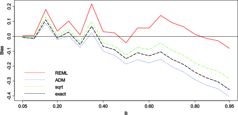
Figure 3: Plot of simulated biases of different GML estimators of $B_{i}$: the balanced case.

The Bayes estimator of $\theta_{i}=x_{i}^{\prime}\beta+u_{i}$, as approximated by the ADM method, is identical to an EBLUP of $\theta_{i}$ when the ALM estimator of $A$ is used in place of REML, ML or other standard variance component estimators. The results on the frequentist coverage (i.e., conditional on the hyperparameters $\beta$ and $A$) of the approximate Bayesian intervals of $\theta_{i}$ presented in the Morris–Tang paper should be encouraging to the non-Bayesians. However, from a frequentist perspective, the interesting problem of establishing the second-order accuracy of coveragealong the lines of Li and Lahiri (2010) remains open. Morris and Tang suggested an approximation to the posterior variance of $\theta_{i}$ as a measure of uncertainty of their point estimate. However, since their point estimate of $\theta_{i}$ can be viewed as an EBLUP, one may suggest the Morris–Tang measure of uncertainty to estimate the traditional mean squared error (same as the integrated Bayes risk, conditional on the hyperparameters) as described in Jiang and Lahiri(2006). It is not, however, clear if the usual second-order unbiasedness criterion, advocated by the non-Bayesians, would be satisfied by the approximate posterior variance formula given in (58) of the Morris–Tang paper. We refer the readers to Rao (2003) and Jiang and Lahiri (2006) for a review of the non-Bayesian methods.

The standard variance component estimation methods such as the REML and ML, despite their good asymptotic properties, frequently yield zero estimates of the unknown variance component $A$. This is a lingering problem in the classical variance component literature. For the model (1)–(2), the simulation results given in Li and Lahiri (2010) suggest that the percentage of zero estimates by the REML method depends on several factors, including the variation of the ratios $V_{i}/A$ across the small areas and the value of $k$. Li and Lahiri (2010) obtained an adjusted maximum likelihood (AML) by multiplying the profile likelihood, as given by $L_{P}(A)$ in Section 2 of Li and Lahiri (2010), by an adjustment factor $A$. This translates to the following adjustment factor:

$$h(A)=A|X^{\prime}D^{-1}_{V+A}X|^{{1}/{2}}$$

for the corresponding residual likelihood, given in Section 2 of Li and Lahiri (2010). Note that $h(A)$ differs from the adjustment factor $A$ suggested in the paper under discussion by an additional factor $|X^{\prime}D^{-1}_{V+A}X|^{{1}/{2}}$.

In the context of estimating the shrinkage factors $B_{i}$, simulation results of Li and Lahiri (2010) indicate lower biases of the shrinkage estimators when the Li–Lahiri adjustment factor is used, where the bias is defined with respect to the marginal distribution of $y$, given the hyperparameters $\bolds{\beta}$ and $A$. In the context of a general linear mixed model, Lahiri and Li (2009) proposed a generalized maximum likelihood (GML) method, which includes ML, REML, ALM and AML methods as special cases. For the model (1)–(2), the GML essentially maximizes$h(A)\times L(A)$ with respect to $A$, where $h(A)$ is a general adjustment factor. This raises an interesting question: how should one choose an adjustment factor $h(A)$ in the GML method?

To fix ideas, we restrict ourselves to the class of adjustment factors of the form $h(A)=A^{q}$. Since $\mathrm{V}(\hat{B}_{i})$ is not affected by $q$, up to the order $o(k^{-1})$ (Lahiri and Li, 2009), it makes sense to choose $q$ that provides good properties in terms of the bias of the estimator. To this end, using Lahiri and Li (2009), we have

$$\frac{\operatorname{Bias}(\hat{B}_{i})}{\mathrm{V}(\hat{B}_{i})}\approx\frac{1}{B_{i}}\biggl{(}1-\frac{q}{1-B_{i}}\biggr{)}.$$

Obviously, $q=1-B_{i}$ is the ideal choice—one that makes the bias/variance ratio nearly zero. While we cannot use this choice since $A$ is unknown, it suggests the range $[0,1]$ for $q$. Interestingly, the REML corresponds to the choice $q=0$ while the Morris–Tang ALM corresponds to the other extreme $q=1$. A compromise choice is $q=0.5$, which corresponds to $B_{i}=0.5$. In the Bayesian language, this choice would then correspond to the prior $\pi(A)=1/\sqrt{A}$, a prior also mentioned in the paper, since the Morris–Tang ADM recommends the adjustment factor $A$ for any prior on $A$. Figure 3 displays the simulated biases of different estimators of the shrinkage factor for the balanced version of model (1)–(2). In terms of the bias, the multiplier $\sqrt{A}$ usually works better than $A$.

Let us now explain how the ALM or AML method may help a non-Bayesian method like the parametric bootstrap (Chatterjee, Lahiri and Li, 2008; Li and Lahiri, 2010) in constructing intervals for the random effects $\theta_{i}$, which requires repeated generation of a pivotal quantity from several bootstrap samples. A strictly positive estimate of $A$ is absolutely needed for this method since the pivotal quantity is undefined when $A$ estimate is zero. A crude fix is to take a small positive number whenever the estimate of $A$ is zero. But, in a simulation study, Li and Lahiri (2010) observed that the coverage errors and also the length of the parametric bootstrap method could be sensitive to the choice of this positive truncation point. The ALM or AML offers a sensible solution to this problem of the parametric bootstrap method. Li and Lahiri (2010) showed that the use of ALM or AML estimator of $A$ improves on coverage as well as the length of the parametric bootstrap interval estimate.

In the paper under discussion, Morris and Tang discuss the case of a single variance parameter $A$. Pramanik (2008) extended the ADM method to the nested error regression model with two unknown variance components by noting that one of the variance components that corresponds to the within small area variation can be integrated out. However, it is not clear how the ADM method, as proposed by Morris and Tang, would extend to a general linear mixed model with more than two variance components, a situation where a simple method such as the ADM method would be most welcome.

We congratulate the authors for preparing an insightful and informative paper on the ADM method. This will surely inspire others to contribute to this important area of research.

References

- Bell (1999) {barticle}[auto:STB—2011-03-03—12:04:44] \bauthor\bsnmBell, \bfnmW.\binitsW. (\byear1999). \btitleAccounting for uncertainty about variances in small area estimation. In \bjournalBull. Internat. Statist. Inst.: 52nd Session. \bnoteAvailable at http://www.stat.fi/isi99/ proceedings.html. \endbibitem
- Chatterjee, Lahiri and Li (2008) {barticle}[mr] \bauthor\bsnmChatterjee, \bfnmSnigdhansu\binitsS., \bauthor\bsnmLahiri, \bfnmPartha\binitsP. and \bauthor\bsnmLi, \bfnmHuilin\binitsH. (\byear2008). \btitleParametric bootstrap approximation to the distribution of EBLUP and related prediction intervals in linear mixed models. \bjournalAnn. Statist. \bvolume36 \bpages1221–1245. \biddoi=10.1214/07-AOS512, issn=0090-5364, mr=2418655 \endbibitem
- Erkanli (1994) {barticle}[mr] \bauthor\bsnmErkanli, \bfnmAlaattin\binitsA. (\byear1994). \btitleLaplace approximations for posterior expectations when the mode occurs at the boundary of the parameter space. \bjournalJ. Amer. Statist. Assoc. \bvolume89 \bpages250–258. \bidissn=0162-1459, mr=1266297 \endbibitem
- Fay and Herriot (1979) {barticle}[mr] \bauthor\bsnmFay, \bfnmRobert E.\binitsR. E. III and \bauthor\bsnmHerriot, \bfnmRoger A.\binitsR. A. (\byear1979). \btitleEstimates of income for small places: An application of James–Stein procedures to census data. \bjournalJ. Amer. Statist. Assoc. \bvolume74 \bpages269–277. \bidissn=0003-1291, mr=0548019 \endbibitem
- Jiang and Lahiri (2006) {barticle}[mr] \bauthor\bsnmJiang, \bfnmJiming\binitsJ. and \bauthor\bsnmLahiri, \bfnmP.\binitsP. (\byear2006). \btitleMixed model prediction and small area estimation. \bjournalTest \bvolume15 \bpages1–96. \biddoi=10.1007/BF02595419, issn=1133-0686, mr=2252522 \endbibitem
- Kass and Steffey (1989) {barticle}[mr] \bauthor\bsnmKass, \bfnmRobert E.\binitsR. E. and \bauthor\bsnmSteffey, \bfnmDuane\binitsD. (\byear1989). \btitleApproximate Bayesian inference in conditionally independent hierarchical models (parametric empirical Bayes models). \bjournalJ. Amer. Statist. Assoc. \bvolume84 \bpages717–726. \bidissn=0162-1459, mr=1132587 \endbibitem
- Lahiri and Li (2009) {bmisc}[auto:STB—2011-03-03—12:04:44] \bauthor\bsnmLahiri, \bfnmP.\binitsP. and \bauthor\bsnmLi, \bfnmH.\binitsH. (\byear2009). \bhowpublishedGeneralized maximum likelihood method in linear mixed models with an application in small-area estimation. In Proceedings of the Federal Committee on Statistical Methodology Research Conference. Available at http://www.fcsm.gov/events/ papers2009.html. \endbibitem
- Li and Lahiri (2010) {barticle}[mr] \bauthor\bsnmLi, \bfnmHuilin\binitsH. and \bauthor\bsnmLahiri, \bfnmP.\binitsP. (\byear2010). \btitleAn adjusted maximum likelihood method for solving small area estimation problems. \bjournalJ. Multivariate Anal. \bvolume101 \bpages882–892. \biddoi=10.1016/j.jmva.2009.10.009, issn=0047-259X, mr=2584906 \endbibitem
- Otto and Bell (1995) {bmisc}[auto:STB—2011-03-03—12:04:44] \bauthor\bsnmOtto, \bfnmM.\binitsM. and \bauthor\bsnmBell, \bfnmW.\binitsW. (\byear1995). \bhowpublishedSampling error modelling of poverty and income statistics for states. In American Statistical Association, Proceedings of the Section on Government Statistics 160–165. Amer. Statist. Assoc., Alexandria, VA. \endbibitem
- Pramanik (2008) {bmisc}[mr] \bauthor\bsnmPramanik, \bfnmSantanu\binitsS. (\byear2008). \bhowpublishedThe Bayesian and approximate Bayesian methods in small area estimation. Ph.D. thesis, Univ. Maryland, College Park. \bidmr=2717629 \endbibitem
- Rao (2003) {bbook}[mr] \bauthor\bsnmRao, \bfnmJ. N. K.\binitsJ. N. K. (\byear2003). \btitleSmall Area Estimation. \bpublisherWiley, \baddressHoboken, NJ. \biddoi=10.1002/0471722189, mr=1953089 \endbibitem