Computational Complexity of Cyclotomic Fast Fourier Transforms over Characteristic-2 Fields

Abstract

Cyclotomic fast Fourier transforms (CFFTs) are efficient implementations of discrete Fourier transforms over finite fields, which have widespread applications in cryptography and error control codes. They are of great interest because of their low multiplicative and overall complexities. However, their advantages are shown by inspection in the literature, and there is no asymptotic computational complexity analysis for CFFTs. Their high additive complexity also incurs difficulties in hardware implementations. In this paper, we derive the bounds for the multiplicative and additive complexities of CFFTs, respectively. Our results confirm that CFFTs have the smallest multiplicative complexities among all known algorithms while their additive complexities render them asymptotically suboptimal. However, CFFTs remain valuable as they have the smallest overall complexities for most practical lengths. Our additive complexity analysis also leads to a structured addition network, which not only has low complexity but also is suitable for hardware implementations.

1 Introduction

Discrete Fourier transforms (DFTs) [1] have widespread applications in error control codes and cryptography, which in turn are important in almost all digital communication and storage systems. For example, the syndrome decoders of Reed-Solomon codes [2] require DFTs over finite fields to implement the syndrome computation and Chien search efficiently (see, e.g., [3]). Multiplications over GF$(p^{m})$ can also be implemented efficiently by DFTs via the convolution theorem [1] when they are formulated as multiplications of polynomials over GF$(p)$.

Recently, very long DFTs over finite fields are needed in practice. For example, Reed-Solomon codes over GF$(2^{12})$ with thousands of symbols are considered for hard drive and tape storage as well as optical communication systems to increase the data reliability, and the syndrome decoders of such codes require DFTs of lengths up to 4095 over GF$(2^{12})$. However, direct implementations of DFTs have quadratic complexities with the lengths of DFTs, and the computational complexity is prohibitive for the DFTs with thousands of symbols. Therefore we need low-complexity algorithms and efficient hardware implementations for DFTs over finite fields.

The cyclotomic fast Fourier transforms (CFFTs), first proposed in [4], have attracted a lot of attention because of their low multiplicative and overall complexities. Though these advantages of CFFTs have been demonstrated for short to moderate lengths in the literature (see, e.g., [5]), it is unclear if they still hold for large lengths. Therefore asymptotic computational complexity analysis is required to compare the complexities of CFFTs with other existing DFT algorithms over finite fields [6, 7, 8], which can help system designers to find the optimal implementation of very long DFTs.

Another issue regarding the CFFTs is their relatively high additive complexities, which hinder their usages. Though the additive complexities of CFFTs can be reduced by the common expression elimination (CSE) algorithm in [5], the lack of addition network structure increases the difficulty of wiring and module reusing, and introduces other problems to the hardware implementation. Therefore, a structured additive complexity reduction method is appreciated for CFFTs.

In this paper, we analyze the asymptotic computational complexities of CFFTs and derive bounds on the multiplicative and additive complexities of CFFTs. The comparisons between our results and existing algorithms show that CFFTs have the smallest multiplicative complexity, but their high additive complexities render them not asymptotically optimal. However, CFFTs are still valuable as they have the smallest overall complexities for most DFTs with practical lengths. Our additive complexity analysis also leads to a structured addition network, which not only has low complexity but also is suitable for hardware implementations.

2 Cyclotomic Fast Fourier Transforms

To make our paper self-contained, we first review CFFTs over GF$(2^{m})$ [4] briefly in this section. Let $\alpha\in\mbox{GF}(2^{m})$ be an element of order $n$, where $n|2^{m}-1$. Consider an $n$-dimensional vector $\mathbf{f}=(f_{0},f_{1},\cdots,f_{n-1})^{T}$ over GF$(2^{m})$, whose polynomial representation is given by $f(x)=\sum_{i=0}^{n-1}f_{i}x^{i}$. The DFT of $\mathbf{f}$ is $\mathbf{F}=(F_{0},F_{1},\cdots,F_{n-1})^{T}$, where $F_{j}=f(\alpha^{j})$.

We partition the set of integers $\{0,1,\cdots,n-1\}$ into $k$ cyclotomic cosets modulus $n$ with respect to two as:

$$\{0\},\,\{s_{1},2s_{1},\cdots,2^{m_{1}-1}s_{1}\},\,\{s_{2},2s_{2},\cdots,2^{m_{2}-1}s_{2}\},\,\cdots$$

$$\{s_{k-1},2s_{k-1},\cdots,2^{m_{k-1}-1}s_{k-1}\},$$

where $m_{i}$ is the size of the $i$-th cyclotomic coset, and $s_{i}=2^{m_{i}}s_{i}\pmod{n-1}$ is its representative. Then the polynomial $f(x)$ can be decomposed as $f(x)=\sum_{i=0}^{k-1}L_{i}(x^{s_{i}})$, where $L_{i}(y)=\sum_{j=0}^{m_{i}-1}f_{2^{j}s_{i}\,\mathrm{mod}\,n}\,y^{2^{j}}$. The polynomial $L_{i}(x)$ has a property such that $L_{i}(x+y)=L_{i}(x)+L_{i}(y)$, for $x,y\in\textrm{GF}(2^{m})$, which is used to reduce the DFT computational complexity in CFFT.

The element $F_{j}$ in the DFT result $\mathbf{F}$ can be expressed as $F_{j}=f(\alpha^{j})=\sum_{i=0}^{k-1}L_{i}(\alpha^{js_{i}})$. By the normal basis theorem [9], there is a normal basis $\{\gamma_{i}^{2^{0}},\gamma_{i}^{2^{1}},\cdots,\gamma_{i}^{2^{m_{i}-1}}\}$ of GF$(2^{m_{i}})$, such that $\alpha^{s_{i}}\in\mbox{GF}(2^{m})$ can be represented as $\sum_{s=0}^{m_{i}-1}a_{i,j,s}\gamma_{i}^{2^{s}}$, where $a_{i,j,s}$ is binary. Therefore

$$f(\alpha^{j})=\sum_{i=0}^{k-1}\sum_{s=0}^{m_{i}-1}a_{i,j,s}\left(\sum_{t=0}^{m_{i}-1}\gamma_{i}^{2^{s+t\,\mathrm{mod}\,m_{i}}}f_{s_{i}2^{t}\,\mathrm{mod}\,n}\right).$$

Writing in the matrix form, we have that the DFT can be computed by $\mathbf{F}=\mathbf{A}\mathbf{L}\mathbf{f}^{\prime}$, where $\mathbf{f}^{\prime}$ is a rearrangement of $\mathbf{f}$ according to the cyclotomic coset, i.e., $\mathbf{f}^{\prime}=(\mathbf{f}_{0}^{\prime},\mathbf{f}_{1}^{\prime},\cdots,\mathbf{f}_{k-1}^{\prime})^{T}$ with $\mathbf{f}_{i}^{\prime}=(f_{s_{i}},f_{2s_{i}},\cdots,f_{2^{m_{i}-1}s_{i}})$, $\mathbf{A}$ is an $n\times n$ binary matrix accumulating the coefficients $a_{i,j,s}$, and $\mathbf{L}$ is a block diagonal matrix with sub-matrices $\mathbf{L}_{i}$’s on its diagonal. Block $\mathbf{L}_{i}$ is an $m_{i}\times m_{i}$ circulant matrix corresponding to a cyclotomic coset of size $m_{i}$, and it is generated from a normal basis $\{\gamma_{i}^{2^{0}},\gamma_{i}^{2^{1}},\cdots,\gamma_{i}^{2^{m_{i}-1}}\}$ of GF$(2^{m_{i}})$. Therefore, the multiplication between $\mathbf{L}_{i}$ and $\mathbf{f}_{i}^{\prime}$ can be formulated as an $m_{i}$-point cyclic convolution between $\mathbf{b}_{i}=(\gamma_{i}^{2^{0}},\gamma_{i}^{2^{m_{i}-1}},\gamma_{i}^{2^{m_{i}-2}},\cdots,\gamma_{i}^{2^{1}})^{T}$ and $\mathbf{f}_{i}^{\prime}$. Since the matrix $\mathbf{A}$ is binary, the product between $\mathbf{A}$ and the vector $\mathbf{v}=\mathbf{L}\mathbf{f}^{\prime}$ can be simply computed by additions. All the multiplications needed by CFFTs are contributed by the convolutions between $\mathbf{b}_{i}$ and $\mathbf{f}_{i}^{\prime}$. Because the short convolutions can be computed by efficient bilinear algorithms (see, e.g., [1]), CFFTs have very low multiplicative complexities. However, if implemented directly, they will have very high additive complexities.

3 Computational Complexities of CFFTs over Characteristic-2 Fields

In our complexity analysis of CFFTs, we aim to theoretically show that their multiplicative complexities are the smallest among all known techniques and to investigate the optimality of the overall computational complexities of CFFTs. For this effort, we focus on CFFTs of length $n=2^{m}-1$ over GF$(2^{m})$.

We denote the cyclotomic cosets of the set $\{0,1,\cdots,n-1\}$ modulus $n$ with respect to two as $C_{0}$, $C_{1}$, $\cdots$, $C_{k-1}$, and assume that $C_{i}$ has $m_{i}$ elements with a representative $s_{i}$. It is required that $m_{i}$ divides $m$, i.e., $m_{i}|m$. We divide $C_{i}$’s into $d$ groups — $G_{0}$, $G_{1}$, $\cdots$, $G_{d-1}$ — so that $C_{i}$’s in each group are of the same size. We denote the size of $G_{j}$ as $|G_{j}|$.

As described in Sec. 2, an $n$-point CFFT is given by $\mathbf{AL}\mathbf{f}^{\prime}$, where the matrix $\mathbf{A}$ is binary. The product of the matrix $\mathbf{L}$ and the vector $\mathbf{f}^{\prime}$, i.e., a vector $\mathbf{v}=\mathbf{Lf}^{\prime}$, is computed via $k$ cyclic convolutions, with $\mathbf{L}_{i}\mathbf{f}_{i}$ being an $m_{i}$-point cyclic convolution. It is a well-known result that an $n$-point cyclic convolution requires $O(n^{\log_{2}3})$ multiplications and additions, respectively [10]. The $k$ cyclic convolutions contribute to both the multiplicative and additive complexities of the CFFT, while computing $\mathbf{Av}$ only contributes to the additive complexity since $\mathbf{A}$ is binary.

3.1 Multiplicative Complexities of CFFTs over GF$(2^{m})$

By the definition of big $O$ notation, an $m_{i}$-point cyclic convolution has a multiplicative complexity less than $cm_{i}^{\log_{2}3}$, where $c$ is a constant independent with $m_{i}$. Hence the total multiplicative complexity of an $n$-point CFFT is less than $c\sum_{i=0}^{k-1}m_{i}^{\log_{2}3}$. As introduced in the beginning of this section, we can group the cyclotomic cosets according to their sizes into $d$ groups, and each group $G_{j}$ has $|G_{j}|$ cyclotomic cosets. We then have that the size of the cosets in $G_{j}$, given by $g_{j}$, divides $m$, i.e., $g_{j}|m$, and also $d\leq m$. Since $\log_{2}3>1$, we have $\frac{m}{g_{j}}(g_{j})^{\log_{2}3}=m(g_{j})^{\log_{2}\frac{3}{2}}\leq m(m)^{\log_{2}\frac{3}{2}}=m^{\log_{2}3}$. Hence, the total multiplicative complexity satisfies

$$c\sum_{i=0}^{k-1}m_{i}^{\log_{2}3}=c\sum_{j=0}^{d-1}|G_{j}|g_{j}^{\log_{2}3}$$

$$= c\sum_{j=0}^{d-1}\lfloor\frac{|G_{j}|g_{j}}{m}\rfloor\frac{m}{g_{j}}g_{j}^{\log_{2}3}+c\sum_{j=0}^{d-1}(|G_{j}|\bmod m/g_{j})g_{j}^{\log_{2}3}$$

$$\leq 2c\frac{2^{m}-1}{m}m^{\log_{2}3},$$

when $m\geq 4$ since $d\leq m\leq(2^{m}-1)/{m}$ in such cases. Since we are considering the asymptotic complexity, we do not need to consider the case $m<4$. The total multiplicative complexity of an $n$-point CFFT is thus $O(n(\log_{2}n)^{\log_{2}\frac{3}{2}})$ since $m=\log_{2}(n+1)$.

Unfortunately, this bound on multiplicative complexities of CFFTs cannot be generalized to an arbitrary $n$. This can be shown by counterexamples. For instance, for some lengths (say $n=11$ or $13$), the set of integers $\{0,1,\cdots,n-1\}$ is partitioned into only two cyclotomic cosets, $\{0\}$ and $\{1,2,\cdots,n-1\}$. Hence, the total multiplicative complexities of CFFTs of these lengths are on the order of $O(n^{\log_{2}3})$.

3.2 Additive Complexities of CFFTs over GF$(2^{m})$

Both the convolutions and multiplication between the binary matrix $\mathbf{A}$ and the vector $\mathbf{v}=\mathbf{L}\mathbf{f}^{\prime}$ contribute to the additive complexity of an $n$-point CFFT over GF$(2^{m})$ with $n=2^{m}-1$. Since the additive and multiplicative complexities of a cyclic convolution have the same order, the total additive complexity contributed by the convolutions is $O(n(\log_{2}n)^{\log_{2}\frac{3}{2}})$. However, the additive complexities of CFFTs are dominated by the computing $\mathbf{Av}$. Since $\mathbf{A}$ consists of only $0$ and $1$, only addition is needed to compute $\mathbf{Av}$. We will derive the additive complexity of $\mathbf{A}\mathbf{v}$.

The Four-Russian algorithm [11] is an efficient algorithm for binary matrix multiplication, and it requires $O(n^{2}/\log_{2}n)$ additions for a multiplication between an $n\times n$ matrix and an $n$-dimensional vector, referred to as $n\times n$ matrix vector product (MVP). However, it does not consider the structure of $\mathbf{M}$. Next we further reduce the additive complexity of computing $\mathbf{A}\mathbf{v}$ by exploring the inner structure of the matrix $\mathbf{A}$.

As shown in Sec. 2, for an $n$-point CFFT over GF$(2^{m})$ where $n=2^{m}-1$, the matrix $\mathbf{A}$ can be partitioned into $1\times k$ blocks, and each block $\mathbf{A}_{i}$ is of size $(2^{m}-1)\times m_{i}$, and its row $j$ is the representation of $\alpha^{js_{i}}$ under a normal basis in the field GF$(2^{m_{i}})$, where $\alpha$ is an element in GF$(2^{m})$ of order $n$.

We first rearrange the rows of the matrix $\mathbf{A}$ according to the cyclotomic cosets. The rearrangement will result in a new matrix $\mathbf{A}^{\prime}$, which can be partitioned into $k\times k$ blocks. Each block $\mathbf{A}^{\prime}_{ij}$ is of size $m_{i}\times m_{j}$, and row $t$ in the block $\mathbf{A}^{\prime}_{ij}$ is the representation of $\alpha^{2^{t}s_{i}s_{j}}$ under a normal basis in GF$(2^{m_{j}})$. By the property of normal bases, we know that row $t$ is just a right cyclic shift of the previous row, and hence $\mathbf{A}^{\prime}_{ij}$ is a cyclic matrix [12]. We then partition the vector $\mathbf{v}$ into $k$ blocks correspondingly, and the block $\mathbf{v}_{i}$ has $m_{i}$ elements. The product $\mathbf{Av}$ can be recovered by reordering the elements in the vector $\mathbf{A}^{\prime}\mathbf{v}$.

All those $m_{i}\times m_{j}$ blocks can be extended to $m\times m$ matrices while keeping the cyclic property. Since $m_{i}$ and $m_{j}$ are all factors of $m$, we first partition an $m\times m$ matrix into $\frac{m}{m_{i}}\times\frac{m}{m_{j}}$ blocks of size $m_{i}\times m_{j}$, and then set each block to $\mathbf{A}_{ij}$. The resulting $m\times m$ matrix is still a cyclic matrix. After extending all the blocks to $m\times m$ blocks in this way, we will get a $km\times km$ matrix $\mathbf{A}^{\prime\prime}$. To ensure that we can recover the multiplication result $\mathbf{Av}$, we should also extend each sub-vector $\mathbf{v}_{i}$ to a vector of length $m$ by padding zeros in the end, resulting in a $km$-dimensional vector $\mathbf{v}^{\prime\prime}$. The elements in $\mathbf{A}^{\prime\prime}\mathbf{v}^{\prime\prime}$ corresponding to the extended rows are simply discarded.

To utilize this cyclic sub-matrices structure, we construct a new matrix $\mathbf{B}$ and a new vector $\mathbf{u}$ from $\mathbf{A}^{\prime\prime}$ and $\mathbf{v}^{\prime\prime}$, respectively according to the following rules:

$$B_{i_{2}k+i_{1},j_{2}k+j_{1}}=A^{\prime\prime}_{i_{1}m+i_{2},j_{1}m+j_{2}},\,u_{i_{2}k+i_{1}}=v^{\prime\prime}_{i_{1}m+i_{2}},$$ (1)

where $0\leq i_{1},j_{1}<k$, $0\leq i_{2},j_{2}<m$, $A^{\prime\prime}_{i,j}$, $B_{i,j}$ are the elements in row $i$ and column $j$ in the matrix $\mathbf{A}^{\prime\prime}$ and $\mathbf{B}$, respectively, and $u_{i}$ and $v^{\prime\prime}_{i}$ are the elements at position $i$ in the vector $\mathbf{u}$ and $\mathbf{v}^{\prime\prime}$, respectively. The matrix $\mathbf{B}$ just reorders the rows and columns of $\mathbf{A}^{\prime\prime}$, and reordering the vector $\mathbf{v}^{\prime\prime}$ into $\mathbf{u}$ ensures that the product $\mathbf{Av}$ can be extracted by reordering $\mathbf{Bu}$ without additional computational complexity. Since $\mathbf{A}^{\prime\prime}$ contains $k\times k$ blocks of cyclic matrices of size $m\times m$, the matrix $\mathbf{B}$ is a block-cyclic matrix with $m\times m$ block matrices of size $k\times k$.

Since the result $\mathbf{Av}$ can be extracted from $\mathbf{Bu}$ without any additional computational complexity, the computational complexity of $\mathbf{Bu}$ serves as an upper bound of that of $\mathbf{Av}$. Now let us analyze the computational complexity of $\mathbf{Bu}$. The matrix $\mathbf{B}$ is an $m\times m$ block-cyclic matrix, therefore it can be computed via $O(m^{\log_{2}3})$ multiplications between a $k\times k$ matrix and a $k$-dimensional vector and $O(m^{\log_{2}3})$ additions of two $k$-dimensional vectors [10]. Since the matrix $\mathbf{B}$ is a fixed one, all the additions between $k\times k$ matrices can be precomputed, and it does not contribute to the additive complexity. Applying the Four-Russian algorithm, the multiplication between a $k\times k$ matrix and a $k$-dimensional vector requires $O(k^{2}/\log_{2}k)$ additions. The addition between two $k$-dimensional vectors requires $k$ additions, and hence the total computational complexity can be written as

$$O(m^{\log_{2}3}\frac{k^{2}}{\log_{2}k})+O(m^{\log_{2}3}k)=O(m^{\log_{2}3}\frac{k^{2}}{\log_{2}k}).$$

We need to find out the lower and upper bounds of $k$. Before giving these bounds, let us prove two lemmas.

Lemma 1.

In the cyclotomic cosets of $\{0,1,\cdots,2^{m}-2\}$ modulus $2^{m}-1$ with respect to two, there are at most $(2^{m_{i}}-1)/m_{i}$ cosets with size $m_{i}$, where $m_{i}|m$.

Proof.

Consider the nonzero elements in the finite field GF$(2^{m})$, which can be represented as $\alpha^{j}$ and $\alpha$ is a primitive element in GF$(2^{m})$. By normal basis theorem [9], there is at least one normal basis in GF$(2^{m})$. Let us pick a normal basis $\{\gamma^{2^{0}},\gamma^{2^{1}},\cdots,\gamma^{2^{m-1}}\}$ in GF$(2^{m})$. Each element in GF$(2^{m})$ has an $m$-bit binary vector representation under this basis, i.e., $\alpha^{j}=\sum_{i=0}^{m-1}b_{i}\gamma^{2^{i}}$, and $(b_{m-1}b_{m-2}\cdots b_{0})$ is the vector representation of $\alpha^{j}$.

It is easy to see that the vector representation of $\alpha^{2j}$ is just a left cyclic shift of that of $\alpha^{j}$. Therefore, if an integer $j$ is in the cyclotomic coset $C_{i}$, the vector representation of $\alpha^{j}$ repeats itself after $m_{i}$ shifts, where $m_{i}$ is the size of $C_{i}$. If $m_{i}<m$, then $m_{i}|m$, and the vector representation of $\alpha^{j}$ can be partitioned into $\frac{m}{m_{i}}$ blocks, all of which are identical and have the same size $m_{i}$, otherwise it cannot repeat itself after $m_{i}$ cyclic shifts. Therefore, there are at most $(2^{m_{i}}-1)/m_{i}$ cyclotomic cosets with size $m_{i}$. ∎

Lemma 2.

$2^{m}-1<km<2(2^{m}-1)$, where $m$ is a positive integer and $k$ is the number of the cyclotomic cosets of $\{0,1,\cdots,2^{m}-2\}$ modulus $2^{m}-1$ with respect to two.

Proof.

The lower bound of $km$ comes from the fact that $m$ is the maximum cyclotomic coset size. It suffices to prove the upper bound of $km$.

Without loss of generality, we assume that the group $G_{0}$ contains the cosets with a size of $m$, and other groups contain the cosets with sizes less than $m$. Therefore by Lemma 1 we have

$$km =|G_{0}|m+\sum\nolimits_{j=1}^{d-1}|G_{j}|m$$

$$\leq(2^{m}-1)+m\sum\nolimits_{m_{i}=1,m_{i}|m}^{\lfloor\frac{m}{2}\rfloor}\frac{2^{m_{i}}-1}{m_{i}}$$

$$\leq(2^{m}-1)+m\sum\nolimits_{m_{i}=1}^{\lfloor\frac{m}{2}\rfloor}2^{m_{i}}$$

$$\leq(2^{m}-1)+m(2^{\frac{m+2}{2}}-1).$$ (2)

Consider the function $f(x)=x-2^{\frac{x-2}{2}}$. It is easy to check that $f^{\prime}(x)=1-(0.5\ln 2)2^{\frac{x-2}{2}}<0$ when $x\geq 8$, which means $f(x)$ is strictly decreasing when $x\geq 8$. We can also check that $f(9)<0$, and hence $f(x)\leq f(9)<0$ when $x\geq 9$. Therefore, for an integer $m\geq 9$, we have $f(m)<0$, and $m\leq 2^{\frac{m-2}{2}}$. Substituting this in (2), we have $km\leq(2^{m}-1)+(2^{m}-2^{\frac{m-2}{2}})\leq 2(2^{m}-1)$ when $m\geq 10$. For $m\leq 9$, the lemma can be verified by inspection. ∎

We have shown that the total computational complexity of evaluating $\mathbf{Bu}$ is $O(m^{\log_{2}3}k^{2}/\log_{2}k)$ additions, hence there exists a constant $c$ independent of $m$ and $k$ such that the total computational complexity is less than $cm^{\log_{2}3}k^{2}/\log_{2}k$ additions. By Lemma 2, we have

$$cm^{\log_{2}3}\frac{k^{2}}{\log_{2}k} \leq cm^{\log_{2}3}\frac{4(2^{m}-1)^{2}}{m^{2}(m+\log_{2}\frac{1-2^{-m}}{m})}.$$ (3)

Consider the function $f(x)=2^{x}-2^{-x}-2x$. We can show that $f^{\prime}(x)=(2^{x}+2^{-x})\ln 2-2>0$ when $x\geq 2$, and $f(3)>0$. Therefore, $f(x)>f(3)>0$ when $x\geq 3$, which implies $2^{x}-2^{-x}>2x$. Then we can show that

$$\log_{2}\frac{1-2^{-m}}{m}=\log_{2}2^{-\frac{m}{2}}+\log_{2}\frac{(2^{\frac{m}{2}}-2^{-\frac{m}{2}})}{m}\geq-\frac{m}{2},$$

when $m>6$. Since we are considering the asymptotic complexity, the cases when $m\leq 6$ do not need to be considered. Substituting this result to (3), we have

$$cm^{\log_{2}3}\frac{k^{2}}{\log_{2}k}\leq cm^{\log_{2}3}\frac{8(2^{m}-1)^{2}}{m^{3}}=8c\frac{(2^{m}-1)^{2}}{m^{\log_{2}\frac{8}{3}}}.$$

Since $n=2^{m}-1$, the additive complexity of $\mathbf{Bu}$ as well as $\mathbf{Av}$ is upper bounded by $O(n^{2}/(\log_{2}n)^{\log_{2}\frac{8}{3}})$ and is lower than $O(n^{2}/\log_{2}n)$, the additive complexity of the multiplication between an arbitrary $n\times n$ binary matrix and a vector.

3.3 Discussions

Table 1: Asymptotic complexities of $(2^{m}-1)$-point DFT algorithms and their respective restrictions. All logarithms are base two.

Alg.	Restriction		Complexities
	Fields	Lengths ($n$)	Multiplicative	Additive	Total
Wang [6]	GF$(2^{m})$, $m$ arbitrary	$2^{m}-1$	$O(n(\log n)^{2})$	$O(n(\log n)^{2})$	$O(n(\log n)^{3})$
Cantor [7]	GF$(2^{m})$, $m$ arbitrary	$2^{m}-1$	$O(n^{2})$	$O(n^{2})$	$O(n^{2}\log n)$
Gao [13]	GF$(2^{m})$, $m=2^{K}$	$2^{m}-1$	$O(n\log n\log\log n)$	$O(n\log n\log\log n)$	$O(n(\log n)^{2}\log\log n)$
Mateer [8]	GF$(2^{m})$, $m=2^{K}$	$2^{m}-1$	$O(n\log n)$	$O(n\log n\log\log n)$	$O(n(\log n)^{2})$
CFFTs	GF$(2^{m})$, $m$ arbitrary	$2^{m}-1$	$O(n(\log n)^{\log_{2}\frac{3}{2}})$	$O(n^{2}/(\log n)^{\log_{2}\frac{8}{3}})$	$O(n^{2}/(\log n)^{\log_{2}\frac{8}{3}})$

To evaluate the tightness of our asymptotic bounds, in Fig. 1 we compare our bounds with the actual multiplicative and additive complexities of CFFTs in [5]. In Fig. 1, we scale our bounds so that they match the actual complexities when $n=1023$.

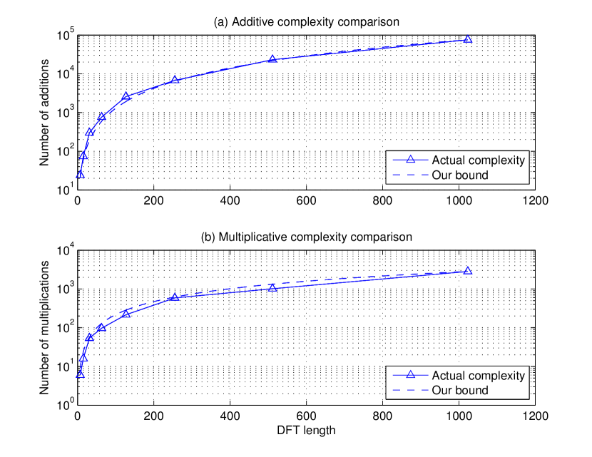
Fig. 1: Comparison of the actual complexities and our bounds.

From Fig. 1, we can see that our bound on additive and the multiplicative complexity is rather tight. The solid curves corresponding to the actual complexities are very closed to the dashed curve corresponding to the theoretical bounds. Therefore, the actual additive and multiplicative complexities are on the order of $O(n^{2}/(\log_{2}n)^{\log_{2}\frac{8}{3}})$ and $O(n(\log_{2}n)^{\log_{2}\frac{3}{2}})$, respectively. We remark that since we have scaled the theoretical bounds to match the actual complexity at certain points, it is not necessary that the computational complexity is strictly smaller than the theoretical bound.

We then compare asymptotic bounds on the complexities of CFFTs and other algorithms in the literature. In [6], a fast DFT algorithm is proposed for GF$(2^{m})$, where $m$ can be any positive integer. Both the additive and multiplicative complexities of this algorithm are of $O(n(\log n)^{2})$. When $m$ is a power of two, more efficient algorithms are proposed. For example, Gao’s algorithm in [13] has both the additive and multiplicative complexities of order $O(n\log n\log\log n)$, and this result is improved by Mateer’s algorithm [8], which reduces the multiplicative complexity to $O(n\log n)$. When the length of the DFT $n=s^{r}$ is a power of some integer $s$, [7] introduces a fast DFT algorithm that has a computational complexity of $rn(s-1)$. Note that this algorithm works for arbitrary algebras rather than finite fields.

Tab. 1 summarizes the asymptotic computational complexities of the aforementioned algorithms when we apply them to the DFTs with lengths of $2^{m}-1$ over GF$(2^{m})$. To compare the total complexities of these algorithms, we define the total complexity to be a weighted sum of the additive and multiplicative complexities, and assume that one multiplication over GF$(2^{m})$ has the same complexity as $2m-1$ additions over the same field. That is, the total complexity is given by $\mbox{total}=(2m-1)\mbox{multiplicative}+\mbox{additive}$. We note that this assumption comes from both the hardware and software considerations [5]. Since we focus on $(2^{m}-1)$-point DFTs, we have that $m=\log_{2}(n+1)$ and $2m-1$ is of order $O(\log n)$.

From Tab. 1, CFFTs have the lowest multiplicative complexities among all algorithms. Furthermore, as shown in Fig. 1(b), our asymptotic bound on the multiplicative complexities of CFFTs is loose. These results confirm the advantage of CFFTs in the multiplicative complexities. On the other hand, due to their high additive complexities, the additive and overall complexities of CFFTs are asymptotically suboptimal. We emphasize the different assumptions for the different DFT algorithms in Tab. 1. For all DFT algorithms, it assumed that the length $n$ and the size of the underlying field are such that a DFT is well-defined. CFFTs and the fast DFT algorithm in [6] have no additional assumptions. In contrast, the other three algorithms in Tab. 1 all have additional constraints. First, Cantor’s algorithm [7] requires $n=s^{r}$, which is often difficult to satisfy. When $n=2^{m}-1$ (and other values of $n$), the only way to satisfy this condition is $n=n^{1}$ due to Mihǎilescu’s Theorem [14]. When $r=1$, Cantor’s algorithm has a quadratic additive and multiplicative complexities and does not have any computational advantage. Furthermore, the algorithms in [8] work only in a field GF$(2^{m})$ with $m=2^{K}$.

As shown in [5], CFFTs have lower overall complexities than all other DFT algorithms for most lengths up to thousands of symbols over GF$(2^{m})$ with $m\leq 12$. The only exception is that for 255-point DFT over GF$(2^{8})$, the overall complexity of Mateer’s algorithm is roughly 4% smaller than a 255-point CFFT. Although the overall complexities of CFFTs are asymptotically suboptimal, CFFTs remain very significant since they have the smallest overall complexities for most practical lengths.

Fig. 2: Implementation diagram of $(2^{m}-1)$-point CFFTs.

4 Hardware Implementations of CFFTs

The architecture of a $(2^{m}-1)$-point CFFT over GF$(2^{m})$ is shown in Fig. 2. First, the input vector $\mathbf{f}$ is reordered and divided into $k$ sub-vectors according to the cyclotomic cosets. Then we perform an $m_{i}$-point cyclic convolution between each sub-vector $\mathbf{f}_{i}^{\prime}$ and its corresponding pre-computed vector $\mathbf{b}_{i}$, as described in Sec. 2. The cyclic convolution results then go through the addition network to compute $\mathbf{Av}$. In Fig. 2, the reordering module can be realized by wiring only and the cyclic convolution modules often can be reused as most of the convolutions are of the same sizes. As the computation of $\mathbf{Av}$ accounts for the majority of the total computational complexity, the addition network in Fig. 2 requires significant area and power in hardware implementations, which makes it difficult to implement CFFTs in hardware. Though the additive complexity of the additive network can be reduced by techniques such as the CSE algorithm in [5], the resulted addition network lacks structure and hence is difficult for hardware implementations.

Fig. 3: Our circuitry for the addition network in Fig. 2. The reordering module has $k$ inputs and $m$ outputs, and the pre-addition module outputs $O(m^{\log_{2}3})$ $k$-dimensional vectors.

Our additive complexity analysis in Sec. 3.2 leads to a structured addition network, which can be implemented by the architecture shown in Fig. 3. The vector $\mathbf{v}$, the cyclic convolution results, is first divided into $k$ sub-vectors according to the sizes of the cyclotomic cosets, and then each sub-vector is extended to $m$-dimensional by padding zeros. The $k$ $m$-dimensional vectors are then reordered into $m$ $k$-dimensional vectors according to (1). Since the addition network follows the bilinear algorithm of an $m\times m$ cyclic convolution, the pre- and post-additions in the bilinear algorithm correspond to the pre-addition and post-addition modules in Fig. 3, respectively, and the multiplications in the bilinear algorithm correspond to the $k\times k$ matrix vector product (MVP) modules, which compute the product between a $k\times k$ binary matrix and a $k$-dimensional vector and can be achieved by simply additions.

The padding and reordering modules in Fig. 3 do not require any logic, and the pre-addition and post-addition have a much smaller complexity than the $k\times k$ MVP modules as shown in Sec. 3. Therefore, the $k\times k$ MVP modules are the primary source of the additive complexity of computing $\mathbf{Av}$. To achieve high throughput, we can implement those $k\times k$ modules in parallel. Furthermore, the CSE algorithm can reduce the additive complexity of each module. Since $k$ is rather small compared with $m$, the CSE algorithm is more effective in simplifying a $k\times k$ MVP than an $m\times m$ one. However, as each module corresponds to a different $k\times k$ matrix, the CSE reduction results are different, and so are the addition networks for each $k\times k$ MVP module. Therefore, those modules must be implemented separately, and we cannot save any chip area by implementing the circuitry in a serial or partly parallel fashion.

Fig. 4: Our circuitry for $k\times k$ MVP modules using the Four-Russian algorithm. LUT stands for “look-up table” and $s=\lceil\log_{2}k\rceil$.

To save area and power, the Four-Russian algorithm [11] can be used to implement the $k\times k$ modules in these cases, using the architecture shown in Fig. 4. According the algorithm, the circuitry has three stages to compute a $k\times k$ MVP, denoted as $\mathbf{Mx}$. The first stage splits $\mathbf{x}$ into $s=\lceil\log_{2}k\rceil$ sub-vectors $\mathbf{x}_{i}$’s, and computes all the binary combinations of elements in each $\mathbf{x}_{i}$. The second stage partitions the matrix $\mathbf{M}$ into $1\times s$ sub-matrices $\mathbf{M}_{i}$’s accordingly, and computes $\mathbf{M}_{i}\mathbf{x}_{i}$ by look-up tables generated from the first stage. Finally the third stage sums up all $\mathbf{M}_{i}\mathbf{x}_{i}$’s. Since the first and last stages in Fig. 4 are independent from $\mathbf{x}$ and $\mathbf{M}$, they can be reused in a serial or partly parallel implementation to save chip area. The second stage depends on $\mathbf{M}$, but it still have a regular structure that is favorable in hardware implementation. No memory or registers are needed in the fully parallel implementation, and buffers used to hold the intermediate results are required in the serial and partly parallel implementation.

In addition to its low complexity, the modular structures of the architectures in Fig. 3 and Fig. 4 are suitable for hardware implementations. First, it is easy to apply architectural techniques such as pipelining to these architectures for better clock rate and throughput. Second, since the $k\times k$ MVP modules account for the majority of the complexity, the modular structure provides various tradeoff options between area, power, and throughput via reusing the $k\times k$ MVP modules in Fig. 3 as well as the combination and select modules in Fig. 4.

References

- [1] R. E. Blahut, Fast Algorithms for Digital Signal Processing. Addison-Wesley, 1985.
- [2] ——, Theory and Practice of Error Control Codes. Addison-Wesley, 1984.
- [3] N. Chen and Z. Yan, “Reduced-complexity Reed-Solomon decoders based on cyclotomic FFTs,” IEEE Signal Process. Lett., vol. 16, no. 4, pp. 279–282, 2009.
- [4] P. V. Trifonov and S. V. Fedorenko, “A method for fast computation of the Fourier transform over a finite field,” Probl. Inf. Transm., vol. 39, no. 3, pp. 231–238, 2003.
- [5] N. Chen and Z. Yan, “Cyclotomic FFTs with reduced additive complexities based on a novel common subexpression elimination algorithm,” IEEE Trans. Signal Process., vol. 57, no. 3, pp. 1010–1020, Mar. 2009.
- [6] Y. Wang and X. Zhu, “A fast algorithm for the Fourier transform over finite fields and its VLSI implementation,” IEEE Journal on Selected Areas in Communications, vol. 6, no. 3, pp. 572–577, Apr. 1988.
- [7] D. G. Cantor and E. Kaltofen, “On fast multiplication of polynomials over arbitrary algebras,” Acta Informatica, vol. 28, pp. 693–701, 1991.
- [8] T. Mateer, “Fast Fourier transform algorithms with applications,” Ph.D. dissertation, Clemson University, 2008.
- [9] R. Lidl and H. Niederreiter, Finite Fields (Encyclopedia of Mathematics and its Applications). Cambridge University Press, October 1996.
- [10] S. Winograd, Arithmetic Complexity of Computations. SIAM, 1980.
- [11] A. V. Aho, J. E. Hopcroft, and J. D. Ullman, The Design and Analysis of Computer Algorithms. Reading, MA: Addison-Wesley, 1974.
- [12] S. V. Fedorenko, “A method for computation of the discrete Fourier transform over a finite fields,” Probl. Inf. Transm., vol. 42, pp. 139–151, 2006.
- [13] S. Gao, “Clemson university mathematical sciences 985 course notes,” Fall 2001.
- [14] P. Mihǎilescu, “Primary cyclotomic units and a proof of Catalan’s conjecture,” Journal für die reine und angewandte Mathematik, vol. 2004, pp. 167 – 195, 2004.