Surface Terms of Quasitopological Gravity and Thermodynamics of Charged Rotating Black Branes

Abstract

We introduce the surface term for quasitopological gravity in order to make the variational principle of the action well-defined. We also introduce the charged black branes of quasitopological gravity and calculate the finite action through the use of the counterterm method. Then we compute the thermodynamic quantities of the black brane solution by use of Gibbs free energy and investigate the first law of thermodynamics by introducing a Smarr-type formula. Finally, we generalize our solutions to the case of rotating charged solutions.

I Introduction

The AdS/CFT conjecture or its stronger version gauge/gravity duality provides a new framework to holographic study of quantum field theory in the nonperturbative regime. According to this duality, the Einstein gravity in the bulk spacetime corresponds to a gauge theory with a large number of colors $N_{c}$ and large ’t Hoof coupling $\lambda$ living on the boundary. Indeed in principle, one can use the dictionary of duality and obtain information on one side by performing computation on the other side Maldacena:1997re . Recently, it has been shown that one can describe strongly coupling phenomena in QCD, condense matter physics and superconductivity by performing gravity calculations. For an interesting review on application in the condense matter physics, see Ref. Hartnoll:2009sz .

The gauge/gravity duality for Einstein gravity with a two-derivative bulk action only works for large $N_{c}$ and large $\lambda$ limit. On the other hand, the coupling constants in the gravity side relate to central charges in the field theory. Thus, Einstein gravity does not have enough free parameters to account for the ratios between central charges and therefore it is only dual to those conformal field theories for which all the central charges are equal. In order to extend the regime of validity to the case of finite $\lambda$ and finite $N_{c}$, or field theories with different ratios between central charges, one should add higher curvature terms or higher derivative terms with more coupling constants within a perturbative framework to action Buchel:2004di ; Myers:2010jv . The first-step generalization is to add the Gauss-Bonnet term to the gravity action. But the Gauss-Bonnet gravity has only one such a coupling constant so the range of its dual theories is limited. In order to extend the duality to new classes of field theories, one can consider terms with higher order curvature interactions such as the third order Lovelock term Hofman:2008ar ; Myers:2010jv . Although the equations of motion of third order Lovelock gravity are second-order differential equations, the third order Lovelock term has no contribution to the field equation in six or lower dimensional spacetime and therefore it is useless for studying field theories in four dimensions. Recently, a new toy model for gravitation action has been proposed which includes cubic curvature interactions and has contribution in five dimensions Myers:2010ru ; Oliva:2010zd . The equations of motion of this theory are second-order differential equations when the metric is spherically symmetry. As in the case of third order Lovelock gravity, the cubic term vanishes in six dimensions. Although this property of Lovelock gravity is due to a topological origin of Euler density in six dimensions, this property of the new theory does not have a topological origin Myers:2010ru . Hence, this theory is known as quasitopological gravity. The black hole solutions and holography study of this toy model have been investigated in Refs. Myers:2010jv ; QTG .

It is known that the Einstein-Hilbert action does not have a well-defined variational principle, since one encounters a total derivative that produces a surface integral involving the derivative of the variation of the metric normal to the boundary. To cancel this normal derivative terms one has to add a surface term to action Gib . Also in the framework of the path integral formalism of quantum gravity, the necessity of adding the surface term has been emphasized Hawking:1979ig . Furthermore, surface terms should be known when one likes to study the general relativity in the Hamiltonian framework York72 . These reasons provide a strong motivation for introducing the surface terms in higher curvature gravity such as Lovelock gravity or quasitopological gravity. The suitable surface term for Lovelock gravity in all orders has been introduced in MDDM . Here, the main aim of this paper is to introduce surface terms for quasitopological gravity in order to have a well-defined variational principle in the case of spacetimes with flat boundary. We also present the static and rotating charged black branes of quasitopological gravity and investigate their thermodynamics. To obtain the conserved quantities of the solutions, we use the counterterm method. This is due to the fact that, as in the case of Einstein gravity, the action and conserved quantities diverge when the boundary goes to infinity. We will introduce a counterterm to deal with these divergences for spacetimes with flat boundary. Since all curvature invariants of the boundary are zero, the only possible boundary counterterm is one proportional to the volume of the boundary regardless of the number of dimensions counterterm .

The outline of our paper is as follows. In Sec. II, we give a brief review of the quasitopological gravity and review the surface terms of the Einstein and Gauss-Bonnet gravities. Then we introduce the surface term of quasitopological gravity for spacetimes with flat boundary. In Sec. III, we introduce asymptotically AdS charged black branes of quasitopological gravity and investigate the thermodynamic properties of these solutions by using the relation between on shell action and Gibbs free energy. Section IV is devoted to the generalization of our static charged solutions to the case of rotating charged solutions. We also study the thermodynamic properties of charged rotating black branes. Finally, we finish our paper with some closing remarks.

II Quasitopological Gravity and Surface Term

The action of quasitopological gravity in $(n+1)$ dimensions with negative cosmological constant $\Lambda=-n(n-1)/2l^{2}$ in the presence of the electromagnetic field may be written as

$$I_{G} = \frac{1}{16\pi}\int_{\mathcal{M}}d^{n+1}x\sqrt{-g}\Big{\{}\frac{n(n-1)}{l^{2}}+R+\frac{\lambda l^{2}}{(n-2)(n-3)}\mathcal{L}_{2}$$ (1)

$$\hskip 42.67912pt+\frac{8(2n-1)\mu l^{4}}{(n-2)(n-5)(3n^{2}-9n+4)}\mathcal{X}_{3}-\frac{1}{4}F_{\mu\nu}F^{\mu\nu}\Big{\}},$$

where $F_{\mu\nu}=\partial_{\mu}A_{\nu}-\partial_{\nu}A_{\mu}$ is the electromagnetic tensor field and $A_{\mu}$ is the vector potential. The first and second terms are the well-known cosmological constant and the Einstein-Hilbert action, the third term is the Gauss-Bonnet term

$$\mathcal{L}_{2}=R_{\mu\nu\gamma\delta}R^{\mu\nu\gamma\delta}-4R_{\mu\nu}R^{\mu\nu}+R^{2},$$ (2)

and the fourth term is the quasitopological term Myers:2010ru

$$\mathcal{X}_{3} = R_{\mu\,\,\nu}^{\,\,\gamma\,\,\,\delta}R_{\gamma\,\,\delta}^{\,\,\sigma\,\,\,\kappa}R_{\sigma\,\,\kappa}^{\,\,\mu\,\,\,\nu}+\frac{1}{(2n-1)(n-3)}\Big{\{}\frac{3(3n-5)}{8}R_{\mu\nu\gamma\delta}R^{\mu\nu\gamma\delta}R$$ (3)

$$-3(n-1)R_{\mu\nu\gamma\delta}R^{\mu\nu\gamma}{}_{\sigma}R^{\delta\sigma}+3(n+1)R_{\mu\nu\gamma\delta}R^{\mu\gamma}R^{\nu\delta}$$

$$+6(n-1)R_{\mu\nu}R^{\nu\gamma}R_{\gamma}{}^{\mu}-\frac{3(3n-1)}{2}RR_{\mu\nu}R^{\mu\nu}+\frac{3(n+1)}{8}R^{3}\Big{\}}.$$

One should note that our coupling constant $\mu$ is $-\mu$ of Ref. Myers:2010ru . Indeed, this term has no contribution to field equations in six or less than five-dimensional spacetimes. But, in contrast to the Lagrangian of third order Lovelock gravity Lov which has no contribution to the field equations in five dimensions, this term contributes to the field equation in five dimensions. The field equations of quasitopological gravity are second-order differential equations only for the case of static metric.

Gibbons and Hawking have mentioned that the Einstein-Hilbert action (with $\lambda=\mu=0$) does not have a well-defined variational principle, since one encounters a total derivative which produces a surface integral involving the derivative of variation of metric normal to the boundary, $\partial_{r}\delta g_{\mu\nu}$. Such terms, which make the variation of action ill defined, should cancel by some surface terms which only depend on the geometry of boundary. In fact, the normal derivative terms can be canceled by the variation of Gibbons-Hawking surface term Gib

$$I_{b}^{(1)}=\frac{1}{8\pi}\int_{\partial\mathcal{M}}d^{n}x\sqrt{-\gamma}K$$ (4)

where $\gamma_{ab}$ is induced metric on the boundary $\partial\mathcal{M}$ and $K$ is the trace of extrinsic curvature of the boundary. Therefore, any generalization of Einstein-Hilbert action needs similar but much more complicated surface terms. However, the surface terms which make the variation of action of Lovelock gravity well-defined are known MDDM . This surface term for the case of Gauss-Bonnet gravity -with $\mu=0$ in the action (1)- is $I_{b}^{(1)}+I_{b}^{(2)}$, where $I_{b}^{(2)}$ is MDDM

$$I_{b}^{(2)}=\frac{1}{8\pi}\int_{\partial\mathcal{M}}d^{n}x\sqrt{-\gamma}\left\{\frac{2\lambda l^{2}}{(n-2)(n-3)}\left(J-2\hat{G}_{ab}^{(1)}K^{ab}\right)\right\}.$$ (5)

In Eq. (5) $\hat{G}_{ab}^{(1)}$ is the $n$-dimensional Einstein tensor of the metric $\gamma_{ab}$, and $J$ is the trace of

$$J_{ab}=\frac{1}{3}(2KK_{ac}K_{b}^{c}+K_{cd}K^{cd}K_{ab}-2K_{ac}K^{cd}K_{db}-K^{2}K_{ab}).$$ (6)

Now, we want to present the surface terms which make the variation of the action of quasitopological gravity (1) well defined. By using the similarity of quasitopological gravity and third order Lovelock gravity, we introduce a surface term which makes the action (1) well defined. For simplification, we restrict our consideration to the case of spacetimes with flat boundary, i.e. $\widehat{R}_{abcd}(\gamma)=0$. Therefore, we suggest a surface term with a combination of fifth order terms in extrinsic curvature as

$$I_{b}^{(3)}=\frac{1}{8\pi}\int_{\partial\mathcal{M}}d^{n}x\sqrt{-\gamma}\Big{\{}\frac{3\mu l^{4}}{5n(n-2)(n-1)^{2}(n-5)}(\alpha_{1}K^{5}$$

$$\,\ \ \ \ \ \ \ \ \ \ \ \ \ \ \ \ \ \ \ \ \ \ \ \ \ \ \ \ +\alpha_{2}K^{3}K_{ab}K^{ab}+\alpha_{3}K_{ab}K^{ab}K_{d}^{c}K_{e}^{d}K_{c}^{e}+\alpha_{4}KK_{b}^{a}K_{a}^{b}K_{d}^{c}K_{c}^{d}$$

$$\,\ \ \ \ \ \ \ \ \ \ \ \ \ \ \ \ \ \ \ \ \ \ \ \ \ \ \ \ +\alpha_{5}KK_{b}^{a}K_{c}^{b}K_{d}^{c}K_{a}^{d}+\alpha_{6}K_{b}^{a}K_{c}^{b}K_{d}^{c}K_{e}^{d}K_{a}^{e}+\alpha_{7}K^{2}K_{b}^{a}K_{c}^{b}K_{a}^{c})\Big{\}}$$ (7)

We can fix the unknown coefficients $\alpha_{i}$ such that all normal derivative of $\delta g_{\mu\nu}$ of quasitopological term are canceled by the variation of $I_{b}^{(3)}$. Since the quasitopological gravity gives second-order differential equations only for the case of static solutions, we present $I_{b}^{(3)}$ for the static metric. The $(n+1)$-dimensional static metric with a flat boundary may be written as

$$ds^{2}=-g(r)dt^{2}+\frac{dr^{2}}{f(r)}+r^{2}\;\sum_{i=1}^{n-1}d\phi_{i}{}^{2}.$$ (8)

Substituting the metric (8) in the action (1) and integrating by parts, we can choose $\alpha_{i}$’s such that the variation of action becomes well defined. One encounters with only five equations for the seven unknown coefficients, $\alpha_{i}$’s. So, one can set two of them to zero, which we choose them to be $\alpha_{6}=\alpha_{7}=0$. It is worth noting that the value of total action is independent of our choice. The values of $\alpha_{i}$’s may be obtained as

$$\alpha_{{1}}=n,\text{ \ \ }\alpha_{{2}}={-2,}\text{ \ \ }\alpha_{{3}}=4(n-1),$$

$$\alpha_{{4}}={-n(5n-6)},\text{ \ \ \ }\alpha_{{5}}={(n-1)(5n-6)}.$$ (9)

In general $I=I_{G}+I_{b}^{(1)}+I_{b}^{(2)}+I_{b}^{(3)}$ is divergent when evaluated on solutions. One way of eliminating such divergence terms is through the use of the background subtraction method subtrac . However for asymptotically AdS solutions, one can instead deal with these divergences by using the counterterm method inspired by AdS/CFT correspondence. In this method the divergence terms are removed by adding a counterterm action $I_{\mathrm{ct}}$ which depends on the boundary curvature invariants. The suitable counterterm for quasitopological gravity is unknown. However, for the case of spacetimes with flat boundary $\hat{R}_{abcd}(\gamma)=0$, one can add a term proportional to the volume of the boundary:

$$I_{\mathrm{ct}}=-\frac{1}{8\pi}\int_{\partial\mathcal{M}}d^{n}x\sqrt{-\gamma}\;\frac{(n-1)}{L_{\mathrm{eff}}},$$ (10)

where $L_{\mathrm{eff}}$ is a scale length factor that depends on $l$, $\mu$, and $\lambda$. Of course, $L_{\mathrm{eff}}$ must reduce to $l$ as $\mu$ and $\lambda$ go to zero.

III Thermodynamics of Charged black Branes

Here, we investigate the thermodynamics of static charged solutions of quasitopological gravity by the counterterm method introduced in the last section. Since we are assuming spherical symmetry, we can obtain the one-dimensional action. Using the static metric (8) with $g(r)=N^{2}(r)f(r)$ and

$$A_{\mu}=h(r)\delta_{\mu}^{0}$$ (11)

for the vector potential, after integration by parts, the one-dimensional action may be written as

$$I_{G}=\frac{1}{16\pi}\int_{\mathcal{M}}d^{n+1}x\left\{\frac{n-1}{l^{2}}N(r)[r^{n-6}(-\mu l^{6}f^{3}+\lambda l^{4}r^{2}f^{2}-r^{4}l^{2}f+r^{6})]^{\prime}+\frac{r^{n-1}}{2N(r)}h^{\prime 2}\right\}$$ (12)

where prime denotes the derivative with respect to $r$. Varying the action with respect to $f(r)$ yields

$$\left(1-2\lambda\frac{l^{2}}{r^{2}}f(r)+3\mu\frac{l^{4}}{r^{4}}f^{2}(r)\right)\frac{dN(r)}{dr}=0,$$ (13)

which shows that $N(r)$ should be a constant which we set equal to $1$. Varying the action with respect to $h(r)$ and substituting $N(r)=1$ gives

$$rh^{\prime\prime}+(n-1)h^{\prime}=0,$$ (14)

which has the solution

$$h(r)=-\sqrt{\frac{2(n-1)}{n-2}}\frac{q}{r^{n-2}}.$$ (15)

After varying the action (12) with respect to $N(r)$, substituting $N(r)=1$ and using Eq. (15), one obtains

$$1-\Psi+\lambda\Psi^{2}-\mu\Psi^{3}=\frac{ml^{2}}{r^{n}}-\frac{q^{2}l^{2}}{r^{2(n-1)}},$$ (16)

where $\Psi(r)=l^{2}r^{-2}f(r)$ and $m$ is an integration constant. The three roots of cubic Eq. (16) are

$$f_{1}(r) = \frac{r^{2}}{l^{2}}\left(\frac{\lambda}{3\mu}+\alpha+{u}\,{\alpha^{-1}}\right),$$ (17)

$$f_{2,3}(r) = \frac{r^{2}}{l^{2}}\left\{\frac{\lambda}{3\mu}-\frac{1}{2}(\alpha+u\,{\alpha^{-1}})\pm\frac{\sqrt{3}}{2}(\alpha-{u}\,{\alpha^{-1}})\right\},$$ (18)

where

$$u = \frac{\lambda^{2}-3\mu}{9\mu^{2}},\text{ \ }\ \alpha=\left(v+\sqrt{v^{2}-u^{3}}\right)^{1/3},\$$ (19)

$$v = \frac{2\lambda^{3}-9\mu\lambda}{54\mu^{3}}+\frac{1}{2\mu}(1-\frac{ml^{2}}{r^{n}}+\frac{q^{2}l^{2}}{r^{2(n-1)}}).$$ (20)

All of the three roots could be real in the appropriate range of $\mu$ and $\lambda$ Myers:2010ru . For example one can rewrite the last two solutions as

$$f_{2,3}(r)=\frac{r^{2}}{l^{2}}\left\{\frac{\lambda}{3\mu}+\sqrt{u}\left(\cos\frac{\theta}{3}\pm\sqrt{3}\sin\frac{\theta}{3}\right)\right\},$$ (21)

where $\cos{\theta}=vu^{-3/2}$ and $\sin{\theta}=\sqrt{u^{3}-v^{2}}u^{-3/2}$. The second and third solutions are real provided $u^{3}>v^{2}$. In the following, we will consider only the first solution $f_{1}(r)$, which is real every where provided $u^{3}<v^{2}$. This condition reduces to

$$\mu>\frac{\lambda}{3}-\frac{2}{27}\left\{1-\left(1-3\lambda\right)^{3/2}\right\},$$ (22)

which can be satisfied provided $\lambda\leq 1/3$.

One can obtain the temperature of the event horizon by the standard method of analytic continuation of the metric as

$$T=\beta^{-1}=\frac{f^{\prime}(r_{+})}{4\pi}=\frac{n-(n-2)q^{2}l^{2}r_{+}^{2-2n}}{4\pi l^{2}}r_{+},$$ (23)

where $r_{+}$ is the outer horizon radius which is the largest real root of $r_{+}^{2n-2}-ml^{2}\ r_{+}^{n-2}+q^{2}l^{2}=0.$ The solution given in Eq. (17) presents a black hole with two horizons provided $q<q_{\mathrm{ext}}$, an extreme black hole for $q=q_{\mathrm{ext}}$ and a naked singularity if $q>q_{\mathrm{ext}}$, where (see Fig. 1)

$$q_{\mathrm{ext}}=\sqrt{\frac{n}{n-2}}\frac{r_{\mathrm{ext}}^{n-1}}{l}.$$

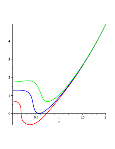
Figure 1: $f(r)$ vs $r$ for $n=4$, $l=1$, $\lambda=0.2$, $\mu=0.03$, $m=0.3$, $q>q_{\mathrm{ext}}$, $q=q_{\mathrm{ext}}$ and $q<q_{\mathrm{ext}}$ from up to down, respectively.

The electric potential $\Phi$, measured at infinity with respect to the horizon, is defined by Gub

$$\Phi=A_{\mu}\xi^{\mu}\mid_{r\rightarrow\infty}-A_{\mu}\xi^{\mu}\mid_{r=r_{+}},$$ (24)

where $\xi^{\mu}$ is the null generator of the horizon. For our static case, $\xi^{\mu}=\delta_{t}^{\mu}$ and therefore one obtains

$$\Phi=\sqrt{\frac{2(n-1)}{n-2}}\frac{q}{r_{+}^{n-2}}.$$ (25)

We calculate entropy, electric charge and mass of this black hole through the use of Gibbs free energy. Following Gib , one can identify the Gibbs free energy function $G$ with the Euclidean action times the temperature, $G=TI_{\mathrm{E}}$. The finite total action, $I_{\mathrm{E}}=I_{\mathrm{g}}+I_{\mathrm{b}}+I_{\mathrm{ct}}$ may be found through the use of the counterterm method introduced in the last section. Straightforward calculations shows that the total Euclidian action is finite provided one sets $L_{\mathrm{eff}}$ in Eq. (10) equal to

$$L_{\mathrm{eff}}=\frac{30\Psi_{1\infty}^{1/2}}{3\mu\Psi_{1\infty}^{3}-5\lambda\Psi_{1\infty}^{2}+15\Psi_{1\infty}+15}l,$$ (26)

where $\Psi_{1\infty}=\lim_{r\rightarrow\infty}\Psi_{1}(r).$ The finite action per volume is calculated as

$$I_{\mathrm{E}}=-\frac{\beta}{16\pi l^{2}}(r_{+}^{n}+\frac{q^{2}l^{2}}{r_{+}^{n-2}}).$$ (27)

Now using Eqs. (23) and (25), the Gibbs free energy per unit volume in terms of the intensive quantities $T$ and $\Phi$ may be written as

$$G(T,\Phi)=-\frac{1}{16\pi l^{2}}\left(r_{+}^{n}+\frac{n-2}{2(n-1)}l^{2}\Phi^{2}r_{+}^{n-2}\right),\,$$ (28)

where $r_{+}$ in terms of temperature and electric potential is

$$\ \ \ \ \ r_{+}=\frac{2\pi l^{2}}{n}T+2\left[\frac{\pi^{2}l^{4}}{n^{2}}T^{2}+\frac{(n-2)^{2}l^{2}}{8n(n-1)}\Phi^{2}\right]^{1/2}.$$ (29)

The  entropy, charge, and energy per volume of charged black brane may be calculated as

$$S = -\left(\frac{\partial G}{\partial T}\right)_{\Phi}=\frac{1}{4}r_{+}^{n-1},$$ (30)

$$Q = -\left(\frac{\partial G}{\partial\Phi}\right)_{T}=\frac{\sqrt{2(n-1)(n-2)}}{16\pi}q,$$ (31)

$$M = G+TS+\Phi Q=\frac{n-1}{16\pi}m$$ (32)

One may note that the entropy density obtained in Eq. (30) is in agreement with the entropy density calculated in Ref. Myers:2010ru . Also, the charge density of Eq. (31) is the same as the value that can be calculated by use of the Gauss law.

One can also find a Smarr-type formula for energy density as a function of $S$ and $Q$:

$$M(S,Q)=\frac{n-1}{\pi l^{2}}\left[S^{2}+\frac{8\pi^{2}l^{2}}{(n-1)(n-2)}Q^{2}\right](4S)^{(2-n)/(n-1)}.$$ (33)

Now one may regard the parameters $S$ and $Q$ as a complete set of extensive parameters for the energy density $M(S,Q)$ and define the intensive parameters conjugate to $S$ and $Q$. These quantities are the temperature and the electric potential:

$$T=\left(\frac{\partial M}{\partial S}\right)_{Q},\,\ \ \ \ \Phi=\left(\frac{\partial M}{\partial Q}\right)_{S}.$$ (34)

It is a matter of straightforward calculation to show that the intensive quantities calculated by Eq. (34) coincide with Eqs. (23) and (25) found previously. Thus, the thermodynamic quantities calculated in this section satisfy the first law of thermodynamics:

$$dM=TdS+\Phi dQ.$$ (35)

IV $(n+1)$-dimensional Charged Rotating Black Branes

In this section we like to endow our charged static solution with a global rotation. The rotation group in $n$ dimensions is $SO(n)$ and therefore the number of independent rotation parameters is $[n/2]$, where $[x]$ is the integer part of $x$. The metric of a $D$-dimensional asymptotically AdS rotating solution with $k\leq[n/2]$ rotation parameters whose constant $(t,r)$ hypersurface has zero curvature may be written as Awad:2002cz

$$ds^{2} = -N(r)^{2}f(r)\left(\Xi dt-{{\sum_{i=1}^{k}}}a_{i}d\phi_{i}\right)^{2}+\frac{r^{2}}{l^{4}}{{\sum_{i=1}^{k}}}\left(a_{i}dt-\Xi l^{2}d\phi_{i}\right)^{2}$$

$$\ +\frac{dr^{2}}{f(r)}-\frac{r^{2}}{l^{2}}{\sum_{i<j}^{k}}(a_{i}d\phi_{j}-a_{j}d\phi_{i})^{2}+r^{2}\;\sum_{i=k+1}^{n-1}d\phi_{i}{}^{2},$$

$$\Xi^{2} = 1+\sum_{i=1}^{k}\frac{a_{i}^{2}}{l^{2}},$$ (36)

where the angular coordinates are in the range $0\leq\phi_{i}<2\pi$. The periodic nature of $\phi_{i}$ allows the metrics (8) and (36) to be locally mapped into each other but not globally, and so they are distinct Stach . Also the gauge potential for this solution is given by

$$A_{\mu}=-\sqrt{\frac{2(n-1)}{n-2}}\frac{q}{r^{n-2}}\left(\Xi dt-\sum_{i=1}^{k}a_{i}d\phi_{i}\right).$$ (37)

Now, we investigate the thermodynamics of rotating charged black branes. The temperature of the event horizon is given by

$$T=\frac{1}{2\pi}\left(-\frac{1}{2}\nabla_{b}\xi_{a}\nabla^{b}\xi^{a}\right)_{r=r_{+}}^{1/2},$$ (38)

where $\xi$ is the Killing vector

$$\xi=\partial_{t}+\sum_{i=1}^{k}\Omega_{i}\partial_{\phi_{i}}$$ (39)

and $\Omega_{i}$ is the angular velocity of the Killing horizon given as

$$\Omega_{i}=-\left[\frac{g_{t\phi_{i}}}{g_{\phi_{i}\phi_{i}}}\right]_{r=r_{+}}=\frac{a_{i}}{\Xi l^{2}}.$$ (40)

Using Eqs. (38)-(40), one obtains

$$T=\beta^{-1}=\frac{f^{\prime}(r_{+})}{4\pi\Xi}=\frac{n-q^{2}l^{2}(n-2)r_{+}^{2-2n}}{4\pi l^{2}\Xi}r_{+}\,.$$ (41)

The electric potential $\Phi$ can be calculated by use of Eqs. (24) and (39) as

$$\Phi=\sqrt{\frac{2(n-1)}{n-2}}\frac{q}{\Xi r_{+}^{n-2}}.$$ (42)

Again, one may obtain the finite action per volume through the use of the counterterm method as

$$I_{\mathrm{E}}=-\frac{\beta}{16\pi l^{2}}(r_{+}^{n}+\frac{q^{2}l^{2}}{r_{+}^{n-2}}).$$ (43)

Now using Eqs. (40), (41) and 42), the Gibbs free energy per unit volume in terms of the intensive quantities $T$, $\Phi$ and $\Omega_{i}$’s may be written as

$$G(T,\Phi,\mathbf{\Omega})=-\frac{1}{16\pi l^{2}}\left(r_{+}^{n}+\frac{(n-2)l^{2}\Phi^{2}}{2(n-1)(1-l^{2}\mathbf{\Omega}^{2})}r_{+}^{n-2}\right),$$ (44)

where the horizon radius in term of the intensive quantities $T$, $\Phi$ and $\Omega_{i}$’s is

$$r_{+}=(1-l^{2}\mathbf{\Omega}^{2})^{-1/2}\left\{\frac{2\pi l^{2}}{n}T+2\left[\frac{\pi^{2}l^{4}}{n^{2}}T^{2}+\frac{(n-2)^{2}l^{2}}{8n(n-1)}\Phi^{2}\right]^{1/2}\right\}.$$ (45)

Now entropy, charge and energy per volume of rotating charged black brane may be calculated as

$$S = -\left(\frac{\partial G}{\partial T}\right)_{\Phi,\Omega_{i}}=\frac{\Xi}{4}r_{+}^{n-1},$$ (46)

$$Q = -\left(\frac{\partial G}{\partial\Phi}\right)_{T,\Omega_{i}}=\frac{\sqrt{2(n-1)(n-2)}}{16\pi}\Xi q,\,$$ (47)

$$J_{i} = -\left(\frac{\partial G}{\partial\Omega_{i}}\right)_{T,\Phi}=\frac{n}{16\pi}\Xi ma_{i},$$ (48)

$$M = G+TS+\Phi Q+\sum\limits_{i=1}^{k}\Omega_{i}J_{i}=\frac{1}{16\pi}(n\Xi^{2}-1)m.$$ (49)

V Concluding Remarks

The action of quasitopological gravity does not have a well defined variational principle, and therefore one needs to add a surface term in order to cancel the derivative of the variation of the metric normal to the boundary. Also, one needs to know the surface terms in the framework of the path integral formalism of quantum gravity, or if one likes to study the general relativity in Hamiltonian framework. Motivated by these facts, we introduced the surface term that makes the variation of the action well-defined. We also introduced the counterterm to deal with the divergences that appeared in the action and calculated the finite action through the use of the counterterm method. Obtaining the finite action, we presented the Gibbs free energy of static charged black branes as a function of the intensive thermodynamic quantities, temperature, and electric potential. We calculated the thermodynamic quantities $S$, $Q$ and energy  densities of the solution through the use of Gibbs free energy and found that these quantities coincide with their values calculated by the geometrical method. We also showed that these quantities satisfy the first law of thermodynamics by obtaining a Smarr-type formula for energy density as a function of entropy and charge densities.

Next, we generalized the static charged solutions to rotating charged solutions and calculated all the conserved and thermodynamic quantities of these black brane solutions. One may use the boundary term introduced in this paper to consider the thermodynamics of the Lifshitz black brane of quasitopological gravity introduced in BDM .

- (1) J. M. Maldacena, Adv. Theor. Math. Phys. 2, 231 (1998) [Int. J. Theor. Phys. 38, 1113 (1999)]; S. S. Gubser, I. R. Klebanov and A. M. Polyakov, Phys. Lett. B 428, 105 (1998); E. Witten, Adv. Theor. Math. Phys. 2, 253-291 (1998).
- (2) S. A. Hartnoll, Class. Quant. Grav. 26, 224002 (2009).
- (3) R. C. Myers, M. F. Paulos, A. Sinha, J. High Energy Phys. 08 (2010) 035.
- (4) A. Buchel, J. T. Liu and A. O. Starinets, Nucl. Phys. B 707, 56 (2005); Y. Kats and P. Petrov, J. High Energy Phys. 01 (2009) 044; R. C. Myers, M. F. Paulos and A. Sinha, Phys. Rev. D 79, 041901 (2009); A. Buchel, R. C. Myers, M. F. Paulos and A. Sinha, Phys. Lett. B 669, 364 (2008); A. Buchel, R. C. Myers and A. Sinha, J. High Energy Phys. 03 (2009) 084; A. Sinha and R. C. Myers, Nucl. Phys. A 830, 295C (2009).
- (5) D. M. Hofman and J. Maldacena, J. High Energy Phys. 05 (2008) 012; D. M. Hofman, Nucl. Phys. B 823, 174 (2009).
- (6) R. C. Myers and B. Robinson, J. High Energy Phys. 08 (2010) 067.
- (7) J. Oliva, S. Ray, Phys. Rev. D 82, 124030 (2010); J. Oliva, S. Ray, Class. Quant. Grav. 27, 225002 (2010).
- (8) X. -M. Kuang, W. -J. Li, Y. Ling, J. High Energy Phys. 12 (2010) 069; J. -P. Wu, J. High Energy Phys. 07 (2011) 106; X. -M. Kuang, W. -J. Li, Y. Ling, arXiv:1106.0784 [hep-th]; K. B. Fadafan, arXiv:1102.2289 [hep-th].
- (9) G. W. Gibbons, S. W. Hawking, Phys. Rev. D 15, 2752-2756 (1977).
- (10) S. W. Hawking and W. Israel, General Relativity: an Einstein Centenary Survey, Cambridge University Press (1979).
- (11) J. W. York, Jr., Phys. Rev. Lett. 28, 1082 (1972).
- (12) R. C. Myers, Phys. Rev. D 36, 392 (1987); S. C. Davis, ibid. 67, 024030 (2003); M. H. Dehghani and R. B. Mann, Phys. Rev. D 73, 104003 (2006); M. H. Dehghani, N. Bostani and A. Sheykhi, ibid. 73, 104013 (2006).
- (13) M. Henningson and K. Skenderis, J. High Energy Phys. 07 (1998) 023; Fortsch. Phys. 48, 125 (2000); S. Nojiri, S. D. Odintsov, Phys. Lett B 444, 92 (1998); S. Hyun, W. T. Kim and J. Lee, Phys. Rev. D 59, 084020 (1999); V. Balasubramanian and P. Kraus, Commun. Math. Phys. 208, 413 (1999).
- (14) D. Lovelock, J. Math. Phys. 12, 498 (1971); N. Deruelle and L. Farina-Busto, Phys. Rev. D 41, 3696 (1990); G. A. MenaMarugan, ibid. 46, 4320 (1992); 4340 (1992).
- (15) J. D. Brown and J. W. York, Phys. Rev. D 47, 1407 (1993); J. D. Brown, J. Creighton and R. B. Mann, Phys. Rev. D 50, 6394 (1994); I. S. Booth and R. B. Mann, Phys. Rev. D 59, 064021 (1999).
- (16) M. Cvetic and S. S. Gubser, J. High Energy Phys. 04, 024 (1999); M. M. Caldarelli, G. Cognola and D. Klemm, Class. Quantum Grav. 17, 399 (2000).
- (17) A. M. Awad, Class. Quant. Grav. 20, 2827 (2003).
- (18) J. Stachel, Phys. Rev. D 26, 1281 (1982).
- (19) W. G. Brenna, M. H. Dehghani and R. B. Mann, Phys. Rev. D 84, 024012 (2011).