On the mass composition of primary cosmic rays in the energy region $10^{15}-10^{16}$ eV

Abstract

The method of a determination of the Primary Cosmic Ray mass composition is presented. Data processing is based on the theoretical model representing the integral muon multiplicity spectrum as the superposition of the spectra corresponding to different kinds of primary nuclei. The method consists of two stages. At the first stage, the permissible intervals of primary nuclei fractions $f_{i}$ are determined on the base of the EAS spectrum vs the total number of muons ($E_{\mu}\geq$ 235 GeV). At the second stage, the permissible intervals of $f_{i}$ are narrowed by fitting procedure. We use the experimental data on high multiplicity muon events ($n_{\mu}\geq$ 114) collected at the Baksan underground scintillation telescope. Within the framework of three components (protons, helium and heavy nuclei), the mass composition in the region $10^{15}-10^{16}$ eV has been defined: $f_{p}=0.235\pm 0.02$, $f_{He}=0.290\pm 0.02$, $f_{H}=0.475\pm 0.03$.

I Introduction

Up to now the energy spectrum and the mass composition of primary cosmic rays (CR) have been measured by direct methods (on satellites or stratosphere balloons) up to energies of about $E_{\scriptscriptstyle N}\simeq 100$ TeV ($E_{\scriptscriptstyle N}$ is the primary nucleus energy). At higher energies the information about CR is obtained with the help of indirect methods which consist in a measurement of different parameters of extensive air showers (EAS). Parameters relating to the energy spectrum are in rather good agreement between each other $[1-11]$, while the data on the mass composition are inconsistent enough (see table 1).

Table 1: Some parameters of the CR energy spectrum and mass composition obtained in different experiments. The second column shows the publish year and reference.

Detector	Reference	$E_{k}$,PeV	$\gamma_{1}$	$\gamma_{2}$	$<lnA>,(p+\alpha)$
MSU	97,Atra ; Fomi	3	$2.7\pm$	$3.1\pm$	$0.62\rightarrow 0.24\ (p+\alpha)$
EAS - TOP	98,Agli3	3	$2.76\pm 0.03$	$3.19\pm 0.06$	$7.1\rightarrow 8.9\ (A_{eff})$
HEGRA	97,Lind	2	$2.60\pm 0.10$	$3.00\pm 0.15$	$0.60\rightarrow 0.45\ (p+\alpha)$
HEGRA	98,Bern		$2.60\pm 0.10$	$3.00\pm 0.15$	$2.0\rightarrow 2.4\ (<lnA>)$
HEGRA	99,Rohr	3.4	$2.67\pm 0.03$	$3.33\pm 0.40$	$0.55\rightarrow 0.48\ (p+\alpha)$
KASCADE	99,Glasst	4	2.7	3.1	$0.70\rightarrow 0.50\ (p+\alpha)$
CASA - MIA	99,Glas2	3	$2.66\pm 0.02$	$3.00\pm 0.05$	$1.3\rightarrow 3\ \ (<lnA>)$
DICE	00,Sword	3	$2.66\pm 0.02$	$3.00\pm 0.05$	$1.5\rightarrow 0.9\ (<lnA>)$
					$0.60-0.50-0.65\ (p+\alpha)$
CASA -	01,Fowl	2-3	$2.72\pm 0.02$	$2.95\pm 0.02$	0.62 - 0.80 - 0.43 $(p+\alpha)$
- BLANCA					1.7 - 1.0 - 1.4 $(<lnA>)$

To investigate the CR mass composition, the EAS parameters are measured which have to be distinct for EAS produced by different kinds of nuclei. These are the number of muons in EAS  $n_{\mu}$, the maximum depth in atmosphere $X_{m}$, fluctuations of the maximum depth $\sigma(X_{m})$, a steepness of lateral distribution of particles near EAS core $\rho(r)$ etc.

The main problem of indirect methods of CR investigation is that the information about both the energy spectrum and the mass composition must be obtained from the same data sample. This leads hereto that the determination of CR mass composition is very difficult problem. There are numerous and various uncertainties related with an interaction model and methods of measurement of EAS characteristics (having, as a rule, considerable errors) and with the CR energy spectrum. These difficulties lead to large spread of obtained results. In Table 1, the parameters of the CR energy spectrum ($E_{k}$ is the ”knee” energy, $\gamma_{1}$ and $\gamma_{2}$ are slope exponents of the spectrum before and after the ”knee”) and the mass composition ($<lnA>$ is the average logarithm of the number of nucleons in a nucleus, $(p+\alpha)$ is the light nuclei fraction) obtained in different experiments are presented. One can see that the trend to weighting mass composition is violated by results reported in Sword ; Fowl .

In the paper we present a method of the determination of CR mass composition on the base of data on the EAS spectrum vs the total number of high energy muons $I(n_{\mu})$.

The paper is constructed as follows. In Section 2, entry conditions are described. In Section 3, we present the method of the determination of primary nuclei fractions intervals $\Delta f_{i}$, which ensure an agreement with experimental data within the limits of one standard deviation. The realization of the method is shown in Sections 4 and 5. In Section 6, intervals of $\Delta f_{i}$ determined at the first stage are narrowed by fitting procedure. Sections 7 and 8 are Discussion and Conclusion.

II Initial conditions

We shall use the data on high multiplicity muon events ($n_{\mu}\geq$ 114) collected at the Baksan underground scintillation telescope Chud . In Voev the muon multiplicity spectrum (i.e., the number $m$ of muons hitting the facility at unknown position of EAS axis) at $m\geq$ 20 was measured at zenith angles $\theta\leq 20^{o}$. The threshold energy of muons coming from this solid angle is 235 GeV.

It is known, the muon multiplicity spectrum depends on the facility geometry and selection conditions of the experiment. This leads to that multiplicity spectra cannot be compared with each other. It would be better to present the data as a function of some invariant variable which does not depend on experiment conditions. In our opinion, the total number of muons in the EAS, $n_{\mu}$, can be chosen as a such variable.

In papers Nov1 ; Nov2 ; Nov4 we developed the method of recalculation from multiplicity spectrum to the EAS spectrum vs the total number of muons, $I(n_{\mu})$. The formulation of the task is following: let F(m) be the integral multiplicity spectrum obtained at a certain facility. Let us define the parameter $\Delta(m)={\overline{m_{1}}/{n_{\mu}}}$, which is the average fraction of muons hitting the facility in the case when the latter is crossed by $m_{1}\geq m$ muons. Assuming then $n_{\mu}=m/{\Delta(m)}$, we will obtain the integral spectrum of EAS vs the total number of muons

$$I(\geq n_{\mu})=\frac{1}{G(m)}F(m),$$ (1)

here $G(m)$ is the acceptance of the facility for a collection of events with muon multiplicity $\geq m$. (It should be explained that m has to be high enough, for example $m>$ 20.)

The numerical values of parameters $\Delta(m)$ and $G(m)$ calculated in Nov2 ; Nov4 with regard to the real structure of the facility are presented in Table 2. $N(\geq m)$ is the experimental number of events with the muon multiplicity $\geq m$ Voev . Nonmonotony of the $N(\geq m)$ is due to the different exposure time, $T_{rec}$.

Table 2: Numerical values of $\Delta(m)$ and $G(m)$. The error in calculation of $\Delta(m)$ and $G(m)$ does not exceed 2-3$\%$. Non-integer values of m are obtained because of corrections at trajectories reconstruction.

$m$	$N(\geq m)$	$T_{rec}$, $10^{6}$ s	$\Delta(m)$	$G(m)$, $m^{2}\cdot sr$	$n_{\mu}$
21.9	127	1.67	0.280	60.5	78.2
32.9	547	19.33	0.289	57.9	113.9
44.5	270	19.33	0.295	56.6	150.8
56.5	164	19.33	0.299	54.8	188.6
82.1	66	19.33	0.306	53.2	268.2
124.9	49	41.93	0.313	51.6	399.3
211.6	7	41.93	0.319	50.4	663.8

The method developed is universal and allows to combine results obtained in different experiments with muon bundles. In our case we have combined the results reported in Voev and Nov4 ; Nov3 and obtained the EAS spectrum vs the total number of muons in the range $75\leq n_{\mu}\leq 4000$, which corresponds to the primary energy range of $10^{15}\leq E_{\scriptscriptstyle N}\leq 10^{17}$ eV (Fig.1). It should be clarified that the data at $n_{\mu}>$ 2000 are obtained for the muon threshold energy $E_{th}=$ 220 GeV, while the points at $n_{\mu}<$ 700 have $E_{th}=$ 235 GeV which is the threshold energy in the experiment Voev . (We do not recalculate the data to the same threshold energy to avoid additional errors.) In Fig.1, the expected fluxes are calculated for $E_{th}=$ 235 GeV ($n_{\mu}<$ 1000, dotted curves) and $E_{th}=$ 220 GeV ($n_{\mu}>$ 1000, solid and dashed curves). Numbers near curves denote the mass composition variants: 1 is the low energy composition (the nuclei fractions in percentage are 39, 24, 13, 13, 11), 2 is the composition (2). Note there is no normalization in Fig.1.

The data at $n_{\mu}<$ 700 can be used for retrieval of information on the CR mass composition in the region $E_{\scriptscriptstyle N}=10^{15}-10^{16}$ eV. Let us remark here that the data at $m=124.9$ and $m=211.6$ in Voev were obtained with essential systematic errors: according to our estimates, the values of $m$ in these points are underestimated 4% and 10% respectively Nov5 , therefore we restrict ourselves to the data at $m\leq 82$ ($n_{\mu}<$ 270).

Figure 1: Squares are the EAS spectrum vs $n_{\mu}$ (experimental data). The muon threshold energy is $E_{th}=$ 235 GeV if $n_{\mu}<$ 1000 and $E_{th}=$ 220 GeV at $n_{\mu}>$ 1000 Nov1 ; Nov4 . Crosses show the muon multiplicity spectrum obtained in Voev ($m$ and $F(m)$ correspond to the multiplicity spectrum). Solid curves are expected fluxes ($E_{th}=$ 220 GeV) for the case $E_{k}=Z\cdot 3\cdot 10^{15}$ eV, dashed curves – the case $E_{k}=3\cdot 10^{15}$ eV/nucleus. Dotted curves show expected fluxes for the case $E_{k}=Z\cdot 3\cdot 10^{15}$ eV at $E_{th}=$ 235 GeV. Numbers near curves denote the mass composition variants: 1 is the ”standard” (low energy) composition, 2 is the composition (2).

As initial conditions, we use the mass composition obtained by Swordy Sword1 with the help of compilation of results of direct measurements at energies $\simeq$ 100 TeV per nucleus (A is the number of nucleons in a nucleus)

$$\begin{array}[]{c}$p$\hskip 14.22636pt$He$\ \ \ $CNO$\ \ \ $Ne-S$\ \ \ $Fe$\\ A\hskip 22.76219pt1\hskip 19.91692pt4\hskip 22.76219pt14\hskip 19.91692pt28\hskip 14.22636pt\ 56\\ f,\%\ \ 25\hskip 14.22636pt31\hskip 19.91692pt19\hskip 17.07164pt12\hskip 19.91692pt13\\ \end{array}$$ (2)

and the proton flux at the energy $E_{p}=$ 100 TeV measured in the JACEE experiment Asak .

$$D_{p}(100\ TeV)=2.95\times 10^{-10}\ (m^{2}\cdot s\cdot sr\cdot GeV)^{-1}$$ (3)

Then the total flux of nuclei with energy of $E=$ 100 TeV is equal to $D_{tot}=D_{p}/0.25=11.8\times 10^{-10}\ (m^{2}\cdot s\cdot sr\cdot GeV)^{-1}$, that is in a good agreement with the result obtained at Tibet array Amen . In this case, the mass composition at the same energy per nucleon is

$$F(100\ TeV)=\left(\begin{array}[]{c}0.88633\\ 0.10412\\ 0.007584\\ 0.001474\\ 0.000492\end{array}\right)$$ (4)

and the total flux of nuclei with the energy 100 TeV/nucleon is equal to

$$D_{N}(100\ TeV)=\sum_{j}D_{tot}f_{j}A^{-1.7}_{j}=3.329\times 10^{-10}\ (m^{2}\cdot s\cdot sr\cdot GeV)^{-1}.$$ (5)

Our goal is to determine the mass composition evolution (from the composition (2)) into the region $E_{\scriptscriptstyle N}=10^{15}-10^{16}$ eV on the base of data on the multiplicity of high energy muons ($E_{\mu}\geq$ 235 GeV) in EAS (see table 2). To this end, we will use the measured fluxes of multiple muon events with the multiplicity into differential intervals  $n_{\mu i}\leq n_{\mu}\leq n_{\mu(i+1)}$. At the first stage, we determine the permissible intervals of primary nuclei fractions $f_{i}$ which ensure an agreement with experimental data within the limits of one standard deviation (Sections 4 and 5). And then, we refine the results with the help of fitting procedure (Section 6).

To obtain the more certain results we fix the CR energy spectrum, namely we adopt the conservative scenario:
i) the slope change of the spectrum occurs at the same energy per unit charge $E_{k}(Z)=$ 3 PeV$\times Z$,
ii) the spectra of all nuclei kinds have the slope exponents $\gamma_{1}=$ 2.7 before the ”knee” and $\gamma_{2}=$ 3.1 after the ”knee”

$$D_{A}(E)=I_{A}E^{-2.7}(1+E/E_{k}(Z))^{-0.4}.$$ (6)

As is seen from table 1 this scenario is supported by experimental data well enough.

It should be emphasized, we do not attempt to use the data at $n_{\mu}>$ 2000 because the energy spectra of primary nuclei at $E_{\scriptscriptstyle N}>10^{16}$ eV are poorly understood.

III Equations

The flux of events with muon multiplicity $n\geq n_{\mu}$ produced by nuclei with A nucleons can be written in the form

$$I_{A}(n\geq n_{\mu})=\int\limits_{E_{th}(A)}^{\infty}D_{A}(E)P_{A}(E,\ n\geq n_{\mu})dE\ ,$$ (7)

here $D_{A}(E)$ is the differential flux of nuclei of kind A, $P_{A}(E,\ n\geq n_{\mu})$ is the probability that the number of muons (with $E_{\mu}\geq$ 235 GeV) in EAS produced by nucleus ”A” (with energy $E$ per nucleon) is $n\geq n_{\mu}$, $E_{th}(A)$ is the threshold energy of nuclei with A nucleons.

We assume that the multiplicity of muons in EAS is described by the negative binomial distribution $B_{A}(E,\ n)$ (Appendix B), then

$$P_{A}(E,\ n\geq n_{\mu})=\sum_{n\geq n_{\mu}}B_{A}(E,\ n)$$

Taking into account that $D_{A}(E)=D_{N}(E)\times F_{A}(E)$, we rewrite (7) so

$$I_{A}(n\geq n_{\mu i})=\int\limits_{E_{th}(A)}^{\infty}F_{A}(E)D_{N}(E)P_{A}(E,\ n\geq n_{\mu i})dE,$$ (8)

and the flux of events with $n_{\mu i}\leq n_{\mu}\leq n_{\mu(i+1)}$ has the form

$$\begin{array}[]{c}J_{A}(\Delta n_{\mu i})=I_{A}(n\geq n_{\mu i})-I_{A}(n\geq n_{\mu(i+1)})=\int\limits_{E_{th}^{i}(A)}^{\infty}F_{A}(E)D_{N}(E)P_{A}(E,\ n\geq n_{\mu i})dE-\\ -\int\limits_{E_{th}^{i+1}(A)}^{\infty}F_{A}(E)D_{N}(E)P_{A}(E,\ n\geq n_{\mu{i+1}})dE=\overline{F}_{A}R_{iA},\end{array}$$ (9)

where the first index of the matrix $R_{ij}$ points out to muon multiplicity ($n_{\mu i}$) and the second one pertains to a nucleus sort. $\overline{F}_{A}$ is the fraction of nuclei ”A” averaged over the energy region which gives the main contribution in the integral (9) (as is seen in Fig.2, the region is rather narrow). Thus we work in the approximation $F_{j}(E)\simeq\overline{F}_{j}=const$ and will drop the symbol of averaging hereinafter.

A fast decrease of the CR flux with the energy is an important simplifying factor. In consequence, the main contribution to the muon bundles flux at any threshold multiplicity $n_{\mu}$ is originated from nuclei whose energies are in a rather narrow region. In Fig.2, the energy distributions of protons and iron nuclei making a contribution to the flux of events (EAS) with $114\leq n_{\mu}(E_{\mu}\geq 235\ GeV)<151$ are shown. The widths of distributions at half-height are $1745-1150$ TeV for iron nuclei and $4985-2485$ TeV for protons.

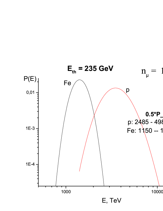
Figure 2: Energy distributions of protons and iron nuclei making a contribution to the flux of muon events with $114\leq n_{\mu}<151$. Areas under curves (p and Fe ) are equal to 1. The widths of distributions at half-height and fractions of events in these regions are indicated.

To avoid possible methodical errors, we use only 4 points in the spectrum $I_{tot}(\geq n_{\mu})\equiv I(\geq n_{\mu})$: at $n_{\mu}=$ 114, 151, 189, 268 (the point at $n_{\mu}=$ 78 has a different exposure time and we do not use it in the present work (see table 2)). In table 3, the input data are presented: muon multiplicity intervals $\Delta n_{\mu}$, the numbers and fluxes of events in given intervals of $n_{\mu}$.

Table 3: Integral ($I$) and finite-difference ($J$) fluxes of events (EAS) with the given number of muons ($E_{\mu}\geq$ 235 GeV). The flux $J(\Delta n_{\mu})$ is defined according to (9).

$n_{\mu}$	$I(\geq n_{\mu})\times 10^{7}$, $(m^{2}\cdot s\cdot sr)^{-1}$	$\Delta n_{\mu}$	$N(\Delta n_{\mu})$	$J\times 10^{7}$, $(m^{2}\cdot s\cdot sr)^{-1}$
114	$4.887\pm 0.209$	114 - 151	277	$2.419\pm 0.145$
151	$2.468\pm 0.150$	151 - 189	106	$0.920\pm 0.089$
189	$1.548\pm 0.121$	189 - 268	98	$0.906\pm 0.092$
268	$0.642\pm 0.079$	$\geq$ 268	66	$0.642\pm 0.079$

We will solve a direct problem and define the regions of $F_{j}$ values which are compatible with equations (couplings)

$$\begin{array}[]{c}\displaystyle\ \ \sum_{j}R_{ij}\times F_{j}=J_{i},\ \ (i=1,2,...,4)\\[14.22636pt] \end{array}$$ (10)

where $J_{i}$ is the observed flux of events with muon multiplicity from $i$-th interval – $n_{\mu i}\leq n_{\mu}<n_{\mu(i+1)}$.

Next we pass to the energy per nucleus and decrease the number of independent variables with the help of relations

$$f_{3}(E)=f_{4}(E)=f_{5}(E),$$ (11)

or

$$f_{3}(E)=1.5f_{4}(E),\ \ f_{4}(E)=f_{5}(E).$$ (12)

where $f_{j}(E)$ is the fraction of nuclei of kind j at the same energy per a nucleus.

The relations (11) are fulfilled at low energies ($E_{\scriptscriptstyle N}\sim$ 100 GeV) and the relations (12) are valid at $E_{\scriptscriptstyle N}\simeq$ 100 TeV (see mass composition (2)). We will find the solution of equations (10) in both cases, and in Section 7 discuss which variant ((11) or (12)) is more preferable.

Thus we work in the approximation $f_{3}(E)\simeq f_{4}(E)\simeq f_{5}(E)$ = 0.1467 and decrease the number of independent variables to three: $f_{1}$, $f_{2}$, $f_{3}$.

Passing from five variables $F_{j}$ to three variables $f_{k}\ (k=1,2,3)$, it is convenient to rewrite the equations (10) as follows (we multiply and divide the j-th term by $A_{j}^{1.7}$ in each equation):

$$\sum_{j=1}^{3}R3_{ij}\times B_{j}=J_{i},\ \ (i=1,2,...,4)$$ (13)

where

$$\begin{array}[]{c}R3_{ij}=R_{ij}/A_{j}^{1.7},\ \ \ B_{j}=F_{j}\times A_{j}^{1.7},\ j=1,2\\ R3_{i3}=\displaystyle\sum_{j=3}^{5}R_{ij}/A_{j}^{1.7},\ \ B_{3}=\displaystyle\frac{1}{3}\sum_{j=3}^{5}F_{j}\times A_{j}^{1.7}.\end{array}$$ (14)

In addition

$$f_{k}=B_{k}\times\displaystyle\left[\sum_{j=1}^{5}F_{j}\times A_{j}^{1.7}\right]^{-1}.$$ (15)

To determine $B_{j}$ we will use independent pairs of equations (13) (for example for i = 1,2 or i = 2,3 etc.), and for closure of the equation system we use the normalization condition

$$f_{1}+f_{2}+3f_{3}=1,$$

which (taking into account (13), (15)) can be read so

$$B_{1}+B_{2}+3B_{3}=\sum_{j=1}^{5}F_{j}\times A_{j}^{1.7}$$ (16)

As it is known, an inverse problem is incorrect (in our case the solution of system (13) is unstable at small variations of fluxes $J_{i}$). Therefore we solve the direct problem, namely: we define the regions of variables $B_{j}$ which result in observed fluxes $J_{i}$ to within one standard deviation $\sigma_{i}=\sqrt{J}_{i}$. In the process we use the mass composition (2) as initial conditions.

IV Permissible domains (I)

In this Section we illustrate the procedure of determination of quantities $B_{j}$ for the first two intervals of muon multiplicity: $\Delta n_{\mu 1}=114-151$ and $\Delta n_{\mu 2}=151-189$ (see table 3).

Let us write the equations (13) for $i=1,2$ in an explicit form

$$\begin{array}[]{l}\displaystyle\sum_{j=1}^{3}R3_{1j}\times B_{j}=J_{1},\\ \displaystyle\sum_{j=1}^{3}R3_{2j}\times B_{j}=J_{2},\end{array}$$ (17)

or in a matrix form

$$R3\_1\times B=J\_1,$$ (18)

where $3\times 3$ matrix R3_1 is composed of elements $R3_{ij}$ for i = 1,2, and the third row of the matrix is the normalization conditions (16)

$$R3\_1=\left(\begin{array}[]{c c c}0.17374&0.38863&2.8885\\ 0.073225&0.16861&1.3701\\ 1&1&3\end{array}\right),$$ (19)

the index _1 means that matrix $R3$ and vector $J$ correspond to the first pair of equations (13). Vector $J\_1$ is by definition (see table 3)

$$J\_1=\left(\begin{array}[]{c}2.419\\ 0.920\\ 3.5453\end{array}\right)$$ (20)

(the third component of $J\_1$ is equal to the sum (16) $\displaystyle J\_1_{3}=\sum_{j=1}^{5}F_{j}\times A_{j}^{1.7}$).

With the help of (13), (14) we get

$$F\rightarrow B^{in}=\left(\begin{array}[]{c}0.88633\\ 1.0991\\ 0.51997\end{array}\right)$$ (21)

where $B^{in}$ are the initial conditions.

Next we see that

$$R3\_1\times B^{in}=\left(\begin{array}[]{c}2.0831\\ 0.9626\\ 3.5453\end{array}\right)$$ (22)

To determine the regions of $B_{j}$, which satisfy the relations (17) we shall make the mass composition heavier (or lighter) $B^{in}\rightarrow B^{cur}$ until the result $R\times B^{cur}=J^{cur}$ fall outside the limits $J_{1}\pm\sigma_{1}$, or $J_{2}\pm\sigma_{2}$, where $\sigma_{1}=\sqrt{J}_{1}$, $\sigma_{2}=\sqrt{J}_{2}$ are the errors of a flux measurement.

The change of the mass composition we shall realize by means of a decrease (or an increase) of the proton fraction $B_{1}\rightarrow B_{1}\mp\delta$ and an increase (or a decrease) of fractions of heavier nuclei $B_{2}\rightarrow B_{2}\pm\delta/4$, $B_{3}\rightarrow B_{3}\pm\delta/4$. Performing this procedure with a small step (for example $\delta=0.005$ ) we define the regions

$$B_{j}^{low}\leq B_{j}\leq B_{j}^{up},$$

which provide the fulfillment of the conditions (17) within one standard deviation.

The conditions

$$J_{1}-\sigma_{1}\leq J^{cur}_{1}\leq J_{1}+\sigma_{1},$$ (23)

and

$$J_{2}-\sigma_{2}\leq J^{cur}_{2}\leq J_{2}+\sigma_{2}.$$ (24)

define different regions of $B_{j}$, of course. As we work in the approximation of a slow change of the mass composition, one should choose an intersection of the regions as the solution for the mass composition averaged over the energy region under discussion ( $1170\leq E_{Fe}\leq 2090$ TeV, $2610\leq E_{p}\leq 5840$ TeV, see Fig. 3).

Note the choice of the common region for solution of equations (17) means the use of two experimental points simultaneously. This reduces an influence of experimental errors.

Figure 3: Energy distributions of protons and iron nuclei making a contribution to the flux of muon events with $114\leq n_{\mu}<189$. Areas under curves (p and Fe ) are equal to 1. The widths of distributions at half-height and fractions of events in these regions are indicated.

It should be noted that the regions of $B_{j}$ values defined by (23), (24) may be disjoint at all. This would mean that either i) the mass composition is changed very rapidly (and our approximation $\overline{F}_{j}\simeq const$ is incorrect), or ii) experimental data have such large errors which do not allow the simultaneous fulfillment of the conditions (23), (24). The latter variant is more plausible and this should keep in mind in what follows.

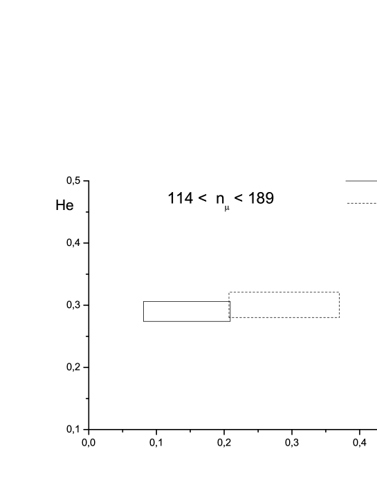
Figure 4: Permissible domains for the protons and He nuclei fractions according to the first pair of equations (13), $i=1,2$.

Solving equations (17) ($i=1,2$) for the conditions (23) we obtain (we present the results for variables $f_{i}$, according to (15)):

$$\begin{array}[]{c}0.0808\leq f_{1}\leq 0.209\\ 0.274\leq f_{2}\leq 0.306\\ 0.172\leq f_{3}\leq 0.205\end{array}$$ (25)

and for conditions (24)

$$\begin{array}[]{c}0.207\leq f_{1}\leq 0.370\\ 0.280\leq f_{2}\leq 0.321\\ 0.117\leq f_{3}\leq 0.158\end{array}$$ (26)

The results are pictorially represented in Fig.4. The intersection of the regions (25) (26) is:

$$\begin{array}[]{c}0.207\leq f_{1}\leq 0.209\\ 0.280\leq f_{2}\leq 0.306\\ 0.172\leq f_{3}\leq 0.158\end{array}$$ (27)

As is obvious, the $f_{3}$ domains disjoint. We discuss a possible reason of that in Section VI. As the temporary solution, we choose the average value – $f_{3}$ = 0.165.

In a similar way, using the second pair of equations (13) for $i=2,3$ ($\Delta n_{\mu 2}=151-189$ and $\Delta n_{\mu 3}=189-268$), we get:

for the condition $J_{2}-\sigma_{2}\leq J^{cur}_{2}\leq J_{2}+\sigma_{2}$

$$\begin{array}[]{c}0.207\leq f_{1}\leq 0.370\\ 0.280\leq f_{2}\leq 0.321\\ 0.117\leq f_{3}\leq 0.158\end{array}$$ (28)

that coincides with (26), certainly, and for the condition $J_{3}-\sigma_{3}\leq J^{cur}_{3}\leq J_{3}+\sigma_{3}$

$$\begin{array}[]{c}0.0808\leq f_{1}\leq 0.271\\ 0.278\leq f_{2}\leq 0.326\\ 0.150\leq f_{3}\leq 0.198\end{array}$$ (29)

The intersection of the regions (28) and (29) (Fig.5) defines the mass composition in the range $151\leq n_{\mu}\leq 268$ ($1630\leq E_{Fe}\leq 3060$ TeV, $3870\leq E_{p}\leq 8750$ TeV):

$$\begin{array}[]{c}0.207\leq f_{1}\leq 0.271\\ 0.280\leq f_{2}\leq 0.321\\ 0.150\leq f_{3}\leq 0.157.\end{array}$$ (30)

Figure 5: Permissible domains for the protons and He nuclei fractions according to the second pair of equations (13), $i=2,3$.

Finally, the third independent pair of equations ($i=3,4$, $\Delta n_{\mu 3}=189-268$ and $\Delta n_{\mu 4}\geq 268$) gives the result (29) for $J_{3}-\sigma_{3}\leq J^{cur}_{3}\leq J_{3}+\sigma_{3}$, and for $J_{4}-\sigma_{4}\leq J^{cur}_{4}\leq J_{4}+\sigma_{4}$

$$\begin{array}[]{c}0.192\leq f_{1}\leq 0.376\\ 0.279\leq f_{2}\leq 0.325\\ 0.115\leq f_{3}\leq 0.161.\end{array}$$ (31)

The intersection of the regions (29) and (31) defines permissible domains for $f_{i}$:

$$\begin{array}[]{c}0.192\leq f_{1}\leq 0.271\\ 0.279\leq f_{2}\leq 0.325\\ 0.150\leq f_{3}\leq 0.161.\end{array}$$ (32)

The widths of energy distributions (at half-height) of iron nuclei and protons making a contribution to the flux of events with $189\leq n_{\mu}\leq 380$ are $2140\leq E_{Fe}\leq 4270$ TeV and $5330\leq E_{p}\leq 12400$ TeV.

V Permissible domains (II)

Now we repeat the calculations of the previous Section using relationships $f_{3}(E)=1.5\times f_{4}(E),\ f_{4}(E)=f_{5}(E)$ instead of (11).

Note that in this case

$$R3_{i3}=\displaystyle R_{i3}/A_{3}^{1.7}+\frac{2}{3}(R_{i4}/A_{4}^{1.7}+R_{i5}/A_{5}^{1.7}),\ \ B_{3}=\displaystyle\frac{3}{7}\sum_{j=3}^{5}F_{j}\times A_{j}^{1.7}.$$ (33)

instead of (14) and the normalization condition reads as follows (compare with (16))

$$B_{1}+B_{2}+\frac{7}{3}B_{3}=\sum_{j=1}^{5}F_{j}\times A_{j}^{1.7}$$ (34)

(We assume $f_{3}(E)=1.5\times f_{4}(E)$ i.e. $F_{3}A_{3}^{1.7}=1.5F_{4}A_{4}^{1.7}$, therefore factors 3/7 and 7/3 appear in (33) and (34))

The matrix R3_1 and vector $B^{in}$ take the form:

$$R3\_1=\left(\begin{array}[]{c c c}0.17374&0.38863&2.1756\\ 0.073225&0.16861&1.0268\\ 1&1&2.3333\end{array}\right),\ \ B^{in}=\left(\begin{array}[]{c}0.88633\\ 1.0991\\ 0.66855\end{array}\right)$$ (35)

Performing the procedure described it the previous Section, we obtain for $i=1,2$
                                            $J_{1}-\sigma_{1}\leq J^{cur}_{1}\leq J_{1}+\sigma_{1}$       $J_{2}-\sigma_{2}\leq J^{cur}_{2}\leq J_{2}+\sigma_{2}$

$$\begin{array}[]{c}0.0554\leq f_{1}\leq 0.185\\ 0.277\leq f_{2}\leq 0.307\\ 0.230\leq f_{3}\leq 0.273\end{array}\hskip 28.45274pt\begin{array}[]{c}0.182\leq f_{1}\leq 0.349\\ 0.287\leq f_{2}\leq 0.326\\ 0.156\leq f_{3}\leq 0.211.\end{array}$$ (36)

The intersection of the regions (36) is

$$\begin{array}[]{c}0.182\leq f_{1}\leq 0.185\\ 0.287\leq f_{2}\leq 0.307\\ 0.230\leq f_{3}\leq 0.211.\end{array}$$ (37)

As with the approximation (11), the $f_{3}$ domains disjoint. We choose the average value $f_{3}$ = 0.220 as the temporary solution. Note within the framework of our approximation $f_{4}=f_{5}=\frac{2}{3}f_{3}$ = 0.147.

Permissible domains for $i=2,3$ $i=3,4$ are:
                                                         $i=2,3$                            $i=3,4$

$$\hskip 28.45274pt\begin{array}[]{c}0.182\leq f_{1}\leq 0.250\\ 0.287\leq f_{2}\leq 0.321\\ 0.203\leq f_{3}\leq 0.211\end{array}\hskip 28.45274pt\begin{array}[]{c}0.160\leq f_{1}\leq 0.250\\ 0.287\leq f_{2}\leq 0.321\\ 0.203\leq f_{3}\leq 0.218.\end{array}$$ (38)

VI Fitting procedure

Thus for the variant (12) $f_{3}(E)=1.5\times f_{4}(E),\ \ f_{4}(E)=f_{5}(E)$ (we shall call it ”Model I”  in the discussion that follows), we have obtained the following permissible domains of $f_{i}$:
                               $i=1,2$                            $i=2,3$                            $i=3,4$

$$\begin{array}[]{c}0.182\leq f_{1}\leq 0.185\\ 0.287\leq f_{2}\leq 0.307\\ f_{3}=0.22\\ f_{4}=f_{5}=0.147\end{array}\hskip 28.45274pt\begin{array}[]{c}0.182\leq f_{1}\leq 0.250\\ 0.287\leq f_{2}\leq 0.321\\ 0.203\leq f_{3}\leq 0.211\\ 0.135\leq f_{4}=f_{5}\leq 0.141\end{array}\hskip 28.45274pt\begin{array}[]{c}0.160\leq f_{1}\leq 0.250\\ 0.287\leq f_{2}\leq 0.321\\ 0.203\leq f_{3}\leq 0.218\\ 0.135\leq f_{4}=f_{5}\leq 0.145\end{array}$$ (39)

and for the variant (11) $f_{3}(E)=f_{4}(E)=f_{5}(E)$ (”Model II”)
                               $i=1,2$                            $i=2,3$                            $i=3,4$

$$\begin{array}[]{c}0.207\leq f_{1}\leq 0.209\\ 0.280\leq f_{2}\leq 0.306\\ f_{3}=0.165\end{array}\hskip 28.45274pt\begin{array}[]{c}0.207\leq f_{1}\leq 0.271\\ 0.280\leq f_{2}\leq 0.321\\ 0.150\leq f_{3}\leq 0.157\end{array}\hskip 28.45274pt\begin{array}[]{c}0.192\leq f_{1}\leq 0.271\\ 0.279\leq f_{2}\leq 0.325\\ 0.150\leq f_{3}\leq 0.161.\end{array}$$ (40)

The obtained results have the status of permissible intervals of fractions $f_{i}$.

The second stage of data processing consists in narrowing of permissible intervals of $f_{i}$. With this end in view, we carry out the simultaneous fit of 4 integral points (see table 3) and 3 finite difference points:

$$\begin{array}[]{c}\displaystyle I_{n_{\mu}}\equiv I(\geq n_{\mu})\ ,\qquad n_{\mu}=114,\quad 151,\quad 189,\quad 268\ ,\\[14.22636pt] \displaystyle J_{n_{\mu}-n^{\prime}_{\mu}}\equiv I(\geq n_{\mu})-I(\geq n^{\prime}_{\mu})\ ,\qquad n_{\mu}-n^{\prime}_{\mu}=114-151,\quad 151-189,\quad 189-268\ .\end{array}$$ (41)

It will be now recalled that for $i=1,2$ the $f_{3}$ domains do not have common region in both variants. This may be associated with experimental errors (see the remark before (25)) at a point (or at some points). It is clear from the general reasoning that the further from reality are experimental points, the smaller is the domain overlap. The smoothing procedure is needed in such a situation.

The analysis has shown that the value of $I(\geq 151)=2.468$ is incompatible with the assumption on a slow change of the mass composition in the energy range under consideration. In the present study we restrict the discussion to the correction of second integral point ($I(\geq 151)=2.468\pm 0.150$) and the more exhaustive analysis will be presented in the later paper. Namely, we increase the second point value by $\frac{1}{2}\sigma$:

$$I(\geq 151)\rightarrow 2.468+0.075=2.543.$$ (42)

This shift results in the common region of $f_{3}$ domains for $i=1,2$ and in so doing the permissible intervals of $f_{i}$ become very close to the ones for $i=2,3$ and $i=3,4$.

Next we perform fitting of 7 points (41) requiring that:
i) all data (7 points) are satisfied within the limits of experimental errors ($\pm 1\sigma$),
ii) fitted parameters ($f_{i}$) are within permissible intervals.

Taking into account (42) the permissible intervals of $f_{i}$ (see (39), (40)) take the form:

$$\begin{array}[]{c}Model\ I:\\[14.22636pt] \displaystyle 0.182\leq f_{p}\leq 0.250\ ,\\[14.22636pt] \displaystyle 0.287\leq f_{He}\leq 0.321\ ,\\[14.22636pt] \displaystyle 0.203\leq f_{N}\leq 0.211\ ,\qquad 0.135\leq f_{Si}=f_{Fe}\leq 0.141\ .\end{array}$$ (43)

$$\begin{array}[]{c}Model\ II:\\[14.22636pt] \displaystyle 0.207\leq f_{p}\leq 0.271\ ,\\[14.22636pt] \displaystyle 0.280\leq f_{He}\leq 0.321\ ,\\[14.22636pt] \displaystyle 0.150\leq f_{N}=f_{Si}=f_{Fe}\leq 0.157\ .\end{array}$$ (44)

In the process of fitting, $f_{He}$ and $f_{N}$ have been chosen as independent fitted parameters. The rest $f_{i}$ are calculated with the help of expressions (12) or (11).

All possible sets of $f_{i}$ for the Model I are presented in Table 4. For each admissible value of $f_{N}$ was found the permissible interval of $f_{He}$. In Table 4, the mean and boundary values of $f_{He}$ are shown for each admissible $f_{N}$. Columns $I_{j},J_{i}$ show the values of the fluxes (41) calculated at given values of $f_{i}$ ($I_{j}$ and $J_{i}$ have to be between min and max values which are shown in the second row). All sets of $f_{i}$ presented in Table are statistically equivalent and can be written as follows:

$$\begin{array}[]{c}\displaystyle f_{p}=0.2365\pm 0.0025\ ,\ f_{He}=0.2895\pm 0.0025\ ,\ f_{N}=0.2038\pm 0.0008\ ,\\[8.53581pt] f_{Si}=f_{Fe}=0.1356\pm 0.0007\ .\end{array}$$ (45)

The fractions of light and heavy nuclei are

$$\begin{array}[]{c}\displaystyle f_{light}=f_{p}+f_{He}=0.526\pm 0.005\ ,\qquad f_{heavy}=f_{N}+f_{Si}+f_{Fe}=0.474\pm 0.003\ .\end{array}$$ (46)

Table 4: Possible sets of primary nuclei fractions $f_{i}$ for the Model I

$\chi^{2}$	$f_{p}$	$f_{He}$	$f_{N}$	$f_{Si}$	$f_{Fe}$	$\langle\ln A\rangle$	$I_{114}$	$I_{151}$	$I_{189}$	$I_{268}$	$J_{114-151}$	$J_{151-189}$	$J_{189-268}$
min	0.182	0.287	0.203	0.1353	0.1353		4.678	2.393	1.427	0.563	2.199	0.906	0.815
max	0.250	0.321	0.211	0.1467	0.1467		5.096	2.693	1.669	0.721	2.489	1.084	0.998
0.333	0.239	0.287	0.203	0.135	0.135	1.929	4.788	2.581	1.562	0.707	2.208	1.018	0.855
0.313	0.237	0.290	0.203	0.135	0.135	1.933	4.833	2.605	1.577	0.714	2.228	1.028	0.863
0.333	0.234	0.292	0.203	0.135	0.135	1.936	4.878	2.629	1.592	0.721	2.249	1.038	0.871
0.317	0.237	0.287	0.204	0.136	0.136	1.937	4.845	2.612	1.581	0.716	2.233	1.031	0.865
0.359	0.234	0.290	0.204	0.136	0.136	1.941	4.900	2.641	1.599	0.724	2.259	1.042	0.875
0.339	0.236	0.287	0.2046	0.1364	0.1364	1.941	4.879	2.630	1.593	0.721	2.249	1.038	0.872

In the same manner, we obtain for the Model II:

$$\begin{array}[]{c}\displaystyle f_{p}=0.2405\pm 0.0045\ ,\ f_{He}=0.2985\pm 0.0145\ ,\ f_{N}=f_{Si}=f_{Fe}=0.1535\pm 0.0035\ .\end{array}$$ (47)

$$\begin{array}[]{c}\displaystyle f_{light}=f_{p}+f_{He}=0.539\pm 0.019\ ,\qquad f_{heavy}=f_{N}+f_{Si}+f_{Fe}=0.461\pm 0.010\ .\end{array}$$ (48)

VII Discussion

The procedure used at the first stage is based on the operation with two equations in 2 variables. To do this, it is necessary to set (in addition to a normalization condition) two relations between fractions $f_{i}$. We use the relations (11) or (12). These additional relationships have a phenomenological nature of course.

Note the results obtained at the first stage depend on the initial conditions, but the second stage of data processing cancels this dependence practically.

Let us remark also the method can be used under any energies (for example $E_{\scriptscriptstyle N}>10^{16}$ eV, $n_{\mu}>$ 1000) if the energy spectra of primary nuclei will be known.

In regard to errors of $f_{i}$ determination, it should be noted the following.

Experimental data (4 points of the integral spectrum and 3 points of the finite-difference spectrum constructed from them) are well described by a power function:

$$\begin{array}[]{c}\displaystyle I(n>n_{\mu})=A\cdot(114/n_{\mu})^{m},\hskip 28.45274ptJ(n_{\mu})=A\cdot(m/114)\cdot(114/n_{\mu})^{(m+1)}\\[8.53581pt] A=4.9442\pm 0.1357,\qquad m=2.3695\pm 0.0921.\end{array}$$ (49)

As we can see, the relative error in spectrum parameters is about 4%, while the relative error of the initial experimental data on the integral spectrum is about 5–10%. This decrease of the relative error is due to matching data with the function and its derivative to get the results (49) (A and m), while the initial errors of 5–10% are applicable only to the function.

Taking into account (49), we are sure that correct processing of the experimental data must detect the mass composition with relative errors in fractions $f_{i}$ under 5%. Of course, these errors can be bigger due to additional simplifying assumptions, e.g. MODEL I or MODEL II. In any case, if errors over 5% are indicated in the final result, then the precision of the method used to process the experimental data (i.e. the solution algorithm for the ill-posed problem) is lower than the precision of these data.

We now discuss the results of the paper. Numbers after $\pm$ signs in (45) and (47) are not the fitting errors. These formulas are compact descriptions of restricted domains, whose full description is given in Tables. As for the true errors of $f_{i}$, the situation is as follows. The errors can be computed only after determining ALL solutions, matched with the experimental data via integral and finite difference spectra. The used algorithm is mathematically very rigid, since it requires matching independent solutions of three pairs of equations with the solution of seven equations. This algorithm does not detect all possible solutions but only a part of them. But the algorithm itself is compatible, so it is possible to claim that the permissible intervals of $f_{i}$ are expanded by at most 5% of the determined ones. If we also take into account ambiguity of the interaction model choice (appendix A), then we get the error value about 10%.

In this context MODEL I and MODEL II result in the same results:

$$f_{p}=0.236\pm 0.020,\ f_{He}=0.290\pm 0.020,\ f_{H}=0.474\pm 0.030$$ (50)

In our opinion, MODEL I is more preferred for the following reasons. First, the relations (12) are satisfied for mass composition (2) defined at $E=$ 100 TeV, i.e. in the neighboring energy region. In the second place, the same relations are characteristic for chemical composition of shells of II type supernova stars, which (according to current concepts) are the sources of high energy cosmic rays.

The results presented above are shown in Fig.6. One can see that uncertainty intervals of $f_{i}$ values for the Model I are noticeably less than the ones for the Model II. Possibly this is one more circumstance pointing to the most adequacy of the Model I.

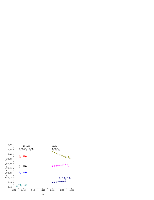
Figure 6: Permissible domains for primary nuclei fractions $f_{i}$.

VIII Conclusion

We have presented the method of retrieval of information on CR mass composition based on a solution of the direct problem (10) with a determination of permissible intervals of primary nuclei fractions $f_{i}$. At the second stage, we constrict the intervals of $f_{i}$ with the help of fitting procedure using the information about the integral spectrum $I(\geq n_{\mu})$ and its derivative $J(\Delta n_{\mu})$.

Data processing is based on the theoretical model representing the integral muon multiplicity spectrum as the superposition of the spectra corresponding to different kinds of primary nuclei. In so doing, it should be kept in mind that we have fixed the interaction model (see appendix A).

With the framework of three components (protons, helium and heavy nuclei) and under the assumption on a slowly change, the CR mass composition in the region $10^{15}-10^{16}$ eV has been defined:

$$f_{p}=0.236\pm 0.020,\ f_{He}=0.290\pm 0.020,\ f_{H}=0.474\pm 0.030$$ (51)

The result (51) should be read as the estimation (rather precise) of CR mass composition in the energy region of $10^{15}-10^{16}$ eV. Thus our analysis points out that CR mass composition become some more heavy in comparison with the one (2).

The method can be used under any energies if the energy spectra of primary nuclei are known.

IX Appendix A

To calculate the parameters $\Delta(m)$ and $G(m)$ Nov1 ; Nov5 , we have used Monte-Carlo simulation and the approximation of spatial-energy distribution function (SDF) of muons in EAS obtained in Bozi ,

$$\hskip 85.35826ptf(r,\geq E,E_{o})=C\times exp{[-(r/r_{o})^{d}]},\hskip 128.0374pt(A.1)$$

here

$$\ \ r_{o}=\frac{0.95}{(1+12.5E)^{0.92}}+\frac{0.42}{E^{1.23}E_{o}^{0.9}},\ \ \ d=0.43+\frac{0.2}{0.2+E_{o}},$$

$E_{o}$ is an energy per nucleon in a primary nucleus, $E$ is the muon threshold energy (E in TeV, r in meters), $C$ - a normalization factor.

The muon density $\rho$ at a distance r from EAS axis is difined by the expression

$$\rho(r,\geq E,E_{o})2\pi rdr=\overline{n}_{\mu}(A,E_{o},\geq E)f(r,E_{o},\geq E)rdr,\hskip 128.0374pt(A.2)$$

here $\overline{n}_{\mu}$ is the average number of muons with energy $\geq E$ produced by a primary nucleus with energy $E_{\scriptscriptstyle N}=AE_{o}$ (A is the number of nucleons in a nucleus) Bozi :

$$\overline{n}_{\mu}(A,E_{o},\geq E,\theta)=\frac{0.0187Y(\theta)A}{{E^{a}}}\left(\frac{E_{o}}{E}\right)^{0.78}\left(\frac{E_{o}}{{E_{o}+E}}\right)^{\delta}\hskip 128.0374pt(A.3)$$

where $E_{o}$ and E in TeV,

$$a=0.9+0.1lg(E),\ \ \delta=E+\frac{11.3}{lg(10+0.5E_{o})},\ \ Y(\theta)=\frac{1+0.36\times ln(\cos\theta)}{\cos\theta}$$

$\theta$ - zenith angle.

X Appendix B

The negative binomial distribution is a discrete probability distribution of the number of successes in a sequence of Bernoulli trials before a specified (non-random) number k of failures occurs

$$\hskip 85.35826ptB(k,p)=C^{r+k-1}_{r}(1-p)^{k}p^{r},\ \ k=0,1,2,...\hskip 128.0374pt(B.1)$$

here $p$ is the probability of success.

Putting $r=n_{\mu}$ and taking into account $\overline{n}_{\mu}=kp/(1-p)$ we obtain

$$\hskip 85.35826ptB(n_{\mu},\overline{n}_{\mu},k)=C^{n_{\mu}+k-1}_{n_{\mu}}\left(\frac{\overline{n}_{\mu}/k}{\overline{n}_{\mu}/k+1}\right)^{n_{\mu}}\frac{1}{(\overline{n}_{\mu}/k+1)^{k}}\hskip 71.13188pt(B.2)$$

The parameter $k$ was chosen in the form obtained in Bozi2

$$\hskip 85.35826ptk=\frac{\overline{n}_{\mu}}{f^{2}-1},\ \ \ f=A^{0.06}\left(1+0.013\frac{E_{o}}{E}\right)^{0.18}\hskip 119.50157pt(B.3)$$

At such choice of $k$ the variance of $B(n_{\mu},\overline{n}_{\mu},k)$ distribution is greater than the one of Poisson distribution in $6-10$ times for protons and $2-3$ times for iron nuclei in the energy region under discussion in accordance with results of others works (e.g. Bilo ; Atta ).

References

- (1) V.B.Atrashkevich et al. Rus.J. Izvestiya of RAS, ser.phys., v.58, N 12, p.45, 1994
- (2) Yu.A. Fomin et al. Proc. 25th ICRC, Durban 4 (1997) 17
- (3) M. Aglietta et al. Astropart. Phys. 10 (1999) 1
- (4) A.Lindner and HEGRA Collaboration. Proc. XXV ICRC, 1997, Durban, v.5, 113
- (5) A.Lindner. Astropart. Phys. 8 (1998) 235
- (6) K.Bernlohr et al. Astropart. Phys. 8 (1998) 253
- (7) A.Rohring et al. Proc. XXVI ICRC, Salt Lake City, 1999, v.1, 214
- (8) R. Glasstetter et al. Proc. XXVI ICRC, Salt Lake City, 1999, v.1, 222
- (9) M.A.K. Glasmacher et al. Astropart. Phys. 12 (1999) 1
- (10) S.P.Swordy, D.B.Kieda. Astropart. Phys. 13 (2000) 137
- (11) J.W. Fowler et al. Astropart. Phys. 15 (2001) 49
- (12) Alexeev E.N. et al., Proc. 16th ICRC, Kyoto, 1979, v. 10, p.276.
- (13) A.V. Voevodsky at al., Rus.J. Izvestiya of RAS, ser.phys., v.58, N 12, p.127, 1994
- (14) V.N. Bakatanov, Yu.F. Novoseltsev, R.V. Novoseltseva. Astropart. Phys. 12 (1999) 19
- (15) Yu.F. Novoseltsev. Rus.J. Nuclear Physics, v.63, N 6, p.1129, 2000
- (16) V.N. Bakatanov, Yu.F. Novoseltsev, R.V. Novoseltseva. Proc. 27th ICRC, Hamburg 2001, v.1, p.84
- (17) V.N. Bakatanov, Yu.F. Novoseltsev, R.V. Novoseltseva. Astropart. Phys. 8 (1997) 59
- (18) Yu.F. Novoseltsev. Doctor of Sciences Thesis, Institute for Nuclear Research of RAS, Moscow, 2003
- (19) Swordy S.P. Proc. XXIII ICRC, Calgary, 1993, Rapporteur Papers, p.243
- (20) Asakimori K. et al. Proc. XXIV ICRC, Rome, 1995, v.2, p.728
- (21) Amenomori M. et al. Proc. XXIV ICRC, Rome, 1995, v.2, p.736
- (22) S.N. Boziev, A.V. Voevodsky, A.E. Chudakov. Preprint P-0630, Institute for Nuclear Research of RAS, 1989
- (23) Boziev S.N. Sov. J. Nuclear Physics, 52 (1990) 500.
- (24) Bilokon H. et al. Proc. XXI ICRC, 1990, Adelaide, v.9, p.366
- (25) Attallah R. et al. Proc. XXIV ICRC, 1995, Rome, v.1, p.573