Mass assembly of galaxies:

Galaxies accrete their mass by means of both smooth accretion from the cosmic web, and the mergers of smaller entities. We wish to quantify the respective role of these two modes of accretion, which could determine the morphological types of galaxies observed today. Multi-zoom cosmological simulations are used to estimate as a function of time the evolution of mass in bound systems, for dark matter as well as baryons. The baryonic contents of dark matter haloes are studied. Merger histories are followed as a function of external density, and the different ways in which mass is assembled in galaxies and the stellar component accumulated are quantified. We find that most galaxies assemble their mass through smooth accretion, and only the most massive galaxies also grow significantly through mergers. The mean fraction of mass assembled by accretion is 77%, and by mergers 23%. We present typical accretion histories of hundreds of galaxies: masses of the most massive galaxies increase monotonically in time, mainly through accretion, many intermediate-mass objects also experience mass-loss events such as tidal stripping and evaporation. However, our simulations suffer from the overcooling of massive galaxies caused by the neglect of active galaxy nuclei (AGN) feedback. The time by which half of the galay mass has assembled, both in dark matter and baryons, is a decreasing function of mass, which is compatible with the observations of a so-called downsizing. At every epoch in the universe, there are low-mass galaxies actively forming stars, while more massive galaxies form their stars over a shorter period of time within half the age of the universe.

1 Introduction

In the standard $\Lambda$CDM scenario, the first structures to form in the universe are low-mass dark haloes, that progressively merge to produce larger and more massive structures (e.g. Blumenthal et al. 1984). Baryons then infall into the dark potential wells, forming stars and rotationally supported galaxies (Fall & Efstathiou 1980). Merging is considered one of the main mechanisms for assembling mass in galaxies and triggering the formation of new stars (Kauffmann et al. 1993; Baugh et al. 1998).

Dark matter haloes and galaxies grow by both mergers and the accretion of diffuse gas component (smooth accretion). In recent years, advances in computational power have allowed us to study in detail the growth of dark matter haloes, which can be probed by numerical simulations (e.g., Madau et al. 2008; Fakhouri & Ma 2010; Genel et al. 2010; Tillson et al. 2011; Wang et al. 2011), but the role of smooth accretion remains uncertain. Galaxy mass assembly has also been investigated using $N$-body simulations including hydrodynamics (e.g., Murali et al. 2002; Semelin & Combes 2005) and semi-analytical models (SAMs, e.g., White & Frenk 1991; Somerville & Kolatt 1999; Kauffmann et al. 1999; Cole et al. 2000; Hatton et al. 2003; Helly et al. 2003; Bower et al. 2006; Neistein et al. 2006; De Lucia & Blaizot 2007; Cattaneo et al. 2011). Birnboim & Dekel (2003) questioned the necessity of shock heating and found a halo mass threshold of $\simeq 10^{11}\mathrm{M}_{\odot}$ below which the pressure of the shock-heated gas is insufficiently high to bear its own gravity and the pressure of infalling material, and is thus unstable. High resolution simulations based on either particles (Kereš et al. 2005, 2009; Brooks et al. 2009; Faucher-Giguère et al. 2011; van de Voort et al. 2011) or a grid (Ocvirk et al. 2008; Dekel et al. 2009), have emphasised the coexistence of two modes of gas accretion. They have demonstrated that hot accretion is spherical, isotropic, and dominates at low redshift and for massive systems, while the cold mode is anisotropic, coming from filaments, and is most significant for lower mass galaxies and at high redshift. Gas accretion by means of cold streams leads to the formation of clumps in the disc that fall towards the centre of the galaxy and merge to form a spheroid (Dekel et al. 2009; Agertz et al. 2009; Ceverino et al. 2010). High-redshift ($z\simeq 2$) star-forming galaxies (SFGs) have been observed by integral field spectroscopy (Genzel et al. 2006; Förster Schreiber et al. 2009). They seem to contain discs, which is incompatible with major mergers, but are very clumpy. This may indicate that they have a high gas fraction, and is consistent with the theoretical predictions of cold accretion (Dekel et al. 2009). The question now arises of the relative roles of merging and external accretion in galaxy mass assembly and formation, and whether some combinations of these processes can explain the observed anti-hierarchical evolution of galaxies, which is usually called the downsizing process (e.g. Cowie et al. 1996). Through the analysis of cosmological $N$-body and hydro simulations, the main focus of the present paper is to quantify the importance of “smooth accretion” relative to merger rates in the mass assembly of galaxies.

Zoom level	0	1	2	3
$m_{\text{DM}}$ ($\mathrm{M}_{\odot}$)	$7.27\times 10^{10}$	$9.09\times 10^{9}$	$1.14\times 10^{9}$	$1.42\times 10^{8}$
$m_{\text{b}}$ ($\mathrm{M}_{\odot}$)	$1.54\times 10^{10}$	$1.93\times 10^{9}$	$2.41\times 10^{8}$	$3.01\times 10^{7}$
$L_{\text{box}}$ (Mpc)	137.0	68.49	34.25	17.12
$\varepsilon_{\text{soft}}$ (kpc)	50.0	25.0	12.5	6.25
$\mathrm{d}t$ (Myr)	20	10	5	2.5
$\Delta t$ (Gyr)	0.2	0.2	0.2	0.1
$z_{\text{end}}$	0	0	0	0.46

Table 1: Parameters of the multi-zoom simulation used here for the four levels of zoom. $L_{\text{box}}$ is the cube length for level 0 zoom, and the diameter for higher level zoom; $\varepsilon_{\text{soft}}$ is the (comoving) softening parameter; $\mathrm{d}t$ is the timestep; and $\Delta t$ is the separation between two consecutive outputs.

Both $N$-body simulations and SAMs have been used to describe the hierarchical process, by building merging trees tracing the formation of a given structure. The Extended Press-Schechter (EPS) formalism (Bond et al. 1991; Lacey & Cole 1993) has been a remarkably successful approximation to obtain mass distributions and merging histories. However, compared to the results derived from $N$-body simulations, there are fundamental differences, owing to the simple hypotheses of a collapse independent of either the environment, the total mass of the structure, or the shape, although a significant improvement was made by considering ellipsoidal collapse (Sheth et al. 2001; Moreno et al. 2009). The simplifying assumptions consider the hierarchical collapse to be a Markov process independent of the history of merging, while the reality is that it is not. Tracing merging trees from cosmological simulations, although more realistic, is not a trivial task either. Many new algorithms have been developed and published, that have complementary strengths and weaknesses (the Friend-of-Friends algorithm (FOF), Davis et al. 1985, SUBFIND, Springel et al. 2001, AdaptaHOP, Aubert et al. 2004; Tweed et al. 2009, hereafter T09), and each relies on their own definitions and conventions to either avoid anomalies, such as the blending of haloes and the unrealistic resulting histories, or deal with substructures (Sheth 2003; Giocoli et al. 2010). In this paper, we use the AdaptaHOP algorithm to detect dark matter haloes and baryonic galaxies.

Cosmological simulations show strikingly that bound structures are not the main component of the large-scale morphology of the universe, but that the filamentary aspect is instead essential and the smooth component of filaments could contain a large fraction of the mass (both dark matter (DM) and baryons). Several methods have tried to quantify the mass in the various components (Stoica et al. 2005, 2010), or to identify the structure of the filamentary skeleton (Novikov et al. 2006; Sousbie et al. 2009; Aragon-Calvo et al. 2010). It is essential to estimate the smooth accretion mass fraction on any scale in $N$-body simulations, to more clearly understand the relative role of mergers and accretion in galaxy formation. The problem is tightly related to the amount of substructures and their evolution, and requires precise definitions (e.g. Giocoli et al. 2010).

When the initial density fluctuations are expressed by a power-law spectrum $P(k)\propto k^{n}$, the variance of the power spectrum on mass scales $M$ is proportional to $M^{\frac{-(n+3)}{3}}$; the low-mass structures should then collapse first, when $n>-3$. Since this is the case in our universe, hierarchical clustering is expected to occur from bottom up. The fact that low-mass dark haloes are found statistically to be the first to assemble, has been confirmed both in $N$-body simulations or through the EPS formalism (e.g. Lacey & Cole 1993; Roukema et al. 1997).

Their growth is quantified by the mass of the main progenitor, or main sub-halo that will later merge into it. Their epoch of formation can then be defined as the time at which the mass of the main progenitor is half the present mass of the halo. However, it is possible to find the opposite trend, when the number of merged haloes more massive than a fixed $M_{\text{min}}$ is considered. More massive haloes have indeed already assembled most of their mass in terms of substructures more massive than $M_{\text{min}}$, while less massive structures are less advanced at the same epoch (Bower 1991; Neistein et al. 2006). This trend can be called downsizing, which is similarly observed for the dark matter, when a minimum mass $M_{\text{min}}$ is introduced.

Interestingly, and for other reasons, the downsizing observed in the baryonic galaxies is also explained when a halo-mass floor $M_{\text{min}}$, below which accretion is quenched, is introduced (Moreno et al. 2009; Bouché et al. 2010). The cold gas accretion would then be limited to a particular mass interval, the maximum mass being reached when the infalling gas is sufficiently shock-heated. Star formation, linked essentially to the cold gas available for accretion, then occurs only in this narrow mass interval. At early times, the more massive haloes reach this floor earlier, and the mass interval is then crossed more rapidly. Star formation in massive galaxies occurs earlier and over a shorter period of time, as the abundance of their elements indicates. The value of $M_{\text{min}}$ required to account for observations is of the order of $10^{11}$ $\mathrm{M}_{\odot}$ (Bouché et al. 2010). Gas exhaustion can then account for any decline in the star formation activity (e.g. Noeske et al. 2007). However, no physical process can explain the existence of this mass floor. Another possible explanation could be that stars form rapidly in low-mass haloes early in the universe, and that most of these small galaxies then merge to form more massive ones, which are observed to be passively evolving on the red sequence today. In this paper, we wish to test this possible scenario, by analysing $N$-body hydrodynamical multi-zoom simulations.

The numerical techniques and the simulation used are described in § 1. The derivations of the bound structure for both dark matter and baryons are presented in § 3. In § 4, we show physical results of our simulation. § 5 describes the results in terms of the fraction of mass accreted by galaxies from the smooth component versus mergers, the influence of the environment being detailed. Our considerations of downsizing are presented in § 6. The discussion in § 7 compares the various scenarios for explaining the downsizing process, and our conclusions are drawn in § 8.

2 Simulations

2.1 Techniques

We use a multi-zoom simulation based on a TreeSPH code (Hernquist & Katz 1989) that is described in Semelin & Combes (2002). Simulating galaxy formation in a cosmological framework involves a wide dynamical range, to simulate a large enough simulation box and to reach a high resolution. We use here the multi-zoom technique described in SC05. The cosmological parameters used in this simulation are taken from WMAP 3 results $(\Omega_{\text{b}},\Omega_{\text{m}},\Omega_{\Lambda},h,\sigma_{8},n)=(0.042,0.24,0.76,0.73,0.75,0.95)$. We start from an initial low-resolution simulation, referred to as the “level 0 zoom”, consisting of $128^{3}/2$ DM particles and $128^{3}/2$ gas particles, which has mass resolutions of $m_{0,\text{DM}}\simeq 7.2\times 10^{10}$ $\mathrm{M}_{\odot}$ and $m_{0,\text{b}}\simeq 1.54\times 10^{10}$ $\mathrm{M}_{\odot}$ and a force resolution $\varepsilon=50$ kpc, in a cubic box of length $L_{0}=137$ Mpc (comoving). We resimulate a sub-region of the original volume at a higher resolution. Tidal fields and the inflow of particles into and the outflow of particles away from the region of interest are recorded at every timestep, and the resimulation is run with these boundary conditions. At each level, we zoom in by a factor of two, improving the mass resolution by a factor of eight, i.e. a low resolution particle at level $N-1$ zoom becomes eight high resolution particles at level $N$. This technique enables any shape of zoom region, and we chose spherical regions. We used three levels of zoom, and ended with a spherical region of radius $R_{3}=8.56$ Mpc, a mass resolution of $m_{3,\text{b}}=3.01\times 10^{7}$ $\mathrm{M}_{\odot}$, $m_{3,\text{DM}}=1.42\times 10^{8}$ $\mathrm{M}_{\odot}$, and a force resolution $\varepsilon=6.25$ kpc (comoving).

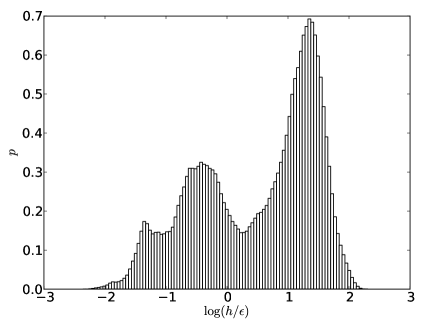
Figure 1: Distribution of the SPH smoothing length $h$ with respect to the gravitational softening parameter $\varepsilon$ at $t=9$ Gyr in the level 3 zoom.

These $128^{3}/2$ particles of mass $m_{0\text{DM}}$ and $m_{0\text{b}}$ at the level 0 give the same mass resolution as a simulation of $128^{3}\times 8^{3}/2=1024^{3}/2$ particles of mass $m_{3\text{DM}}\simeq 1.42\times 10^{8}$ $\mathrm{M}_{\odot}$ and $m_{3\text{b}}\simeq 3.01\times 10^{7}$ $\mathrm{M}_{\odot}$, but focused on a smaller volume of radius 8.56 Mpc at level 3. This technique enable us to simulate galaxies with a fairly high resolution starting with a reasonably sized cosmological box, at a smaller CPU cost.

One of the main characteristics of this technique is that, except at the zeroth level of zoom, the number of particles does not remain constant during the whole simulation. At higher levels of zoom, a particle at timestep $i$ inside the level $N$ box, but outside the level $N+1$ box, can indeed enter the level $N+1$ box at timestep $i+1$ and be split into eight high-resolution particles. Particles with unrecorded history the enter the box, and a special care must be taken when establishing particle identities. Because of this increasing number of particles, the third level of simulations could not be run further than $t=9.1$ Gyr, or $z=0.46$, but lower levels of zoom reached $z=0$.

At the third level of zoom, we end up with 90 snapshots, sampled every 100 Myr from $t=0.2$ Gyr to $t=9.1$ Gyr, which enables us to build the merger tree of structures, while at the three lower levels of zoom we have 70 snapshots, sampled every 200 Myr from $t=0.2$ Gyr to $t=14$ Gyr. The latter can be used for a resolution study (see section 7.1). The properties of each level of zoom are summed up in table 1.

2.2 Physical recipes and initial conditions

While collisionless particles, namely stars and dark matter, undergo only gravitational forces and are treated by a tree algorithm, gas dynamics is treated by smooth particle hydrodynamics (SPH). Additional recipes are needed to mimic subgrid physics such as star formation and feedback. Our physical treatment is described in Semelin & Combes (2002), but the present paper we only use the SPH phase and not the cold and clumpy gas that was described by sticky particles. The SPH gas is treated with the same equation of state and the same viscosity prescription. The range of temperatures is $800-2\times 10^{6}$ K. Any dependance of cooling on metallicity is ignored, and only a primordial metallicity ($10^{-3}$ Z_⊙) is considered. A unique timestep per zoom level is adopted, which is respectively 20, 10, 5, and 2.5 Myr for levels 0 to 3.

The softening length for gravity is respectively 50, 25, 12.5, and 6.25 kpc (comoving), and we checked that the SPH smoothing length is not far shorter than the softening length, as shown on the histogram of Fig. 1 at $t=9$ Gyr in the level 3 zoom.

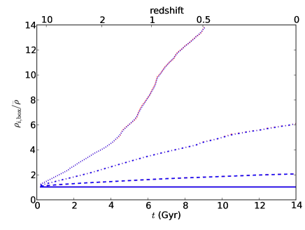
Figure 2: Evolution of the mean comoving density of the box with respect to the cosmic density $\rho_{i,\text{box}}(t)/(\bar{\rho}_{i})$ for the four zoom levels. Level 0 is shown as a solid line, level 1 a dashed line, level 2 dash-dotted and level 3 dotted. The box in the last snapshot a level 3 has a density of 14 times the cosmic density for $i\in$ (DM, baryons).

The radiative cooling term $\Lambda$ is taken from the normalised tables of Sutherland & Dopita (1993) modelling atomic absorption-line cooling from $10^{4}$ K to $10^{8.5}$ K. The background ultraviolet (UV) radiation field is modelled by a constant uniform heating $\Gamma_{\text{UV}}=10^{-24}$ erg s^-1 term.

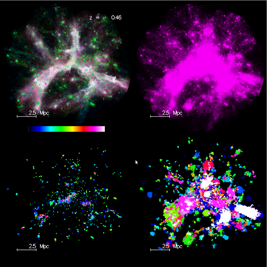
Figure 3: View of the third zoom level of the simulation. Top: Gas (colour-coded by temperature, logarithmic scale from 800 to $1.4\times 10^{6}$ K), and DM (right). Bottom: Structures and substructures detected by AdaptaHOP. Left: baryonic galaxies and satellites, right: DM haloes and subhaloes. Haloes and galaxies are represented in dark and bright blue and green; subhaloes and satellites in yellow, orange, magenta, red, and white. The white bar indicates the comoving length-scale.

Star formation is modelled by a Schmidt law with a star formation rate of

$$\frac{\mathrm{d}{\rho_{*}}}{\mathrm{d}{t}}=C\rho_{\text{gas}}^{n},$$ (1)

with $n=1$. It is applied to gas particles with densities higher than a density threshold of

$$\rho_{\text{min}}=3\times 10^{-2}\,\text{at cm}^{-3}.$$ (2)

Gas particles form stars, and have a fraction of stars within them. When this fraction reaches a given threshold (set to 20%), we search among their neighbours to determine whether there is enough material to form a full star particle, i.e. whether the sum of the star fractions among the neighbouring gas particles is greater than 1. If this is the case, the particle is turned into a star particle, and the fraction of stars in the neighbouring particles becomes gas again. In this way, the stellar fraction within a gas particle remains low, which prevents stars from following the gas dynamics. Kinetic feedback from supernovae (SNe) is also included. Stars more massive than 8 $\mathrm{M}_{\odot}$ are assumed to die as SNe, releasing an energy of $10^{48}$ erg $\mathrm{M}_{\odot}$^-1. The released energy is distributed assuming a Salpeter initial mass function, and an efficiency parameter of 6%. Particles within the smoothing length of the former gas particle receive a velocity kick in the radial direction.

We note that in this study, no AGN feedback is considered, which leads to an overcooling problem and to high stellar masses in the more massive haloes (see § 7.2).

Initial conditions were obtained using Grafic (Bertschinger 2001) at the highest resolution ($1024^{3}$ particles) for level 3, and were then undersampled to build the initial conditions of low-resolution levels.

We ran the level 0 simulation and ran a FOF-like algorithm to detect the haloes to be resimulated. We chose the most massive halo of about $10^{15}\mathrm{M}_{\odot}$ at $z=0$, thus all this work is done in a rich environment. Figure 2 shows the evolution of the mean density, normalised by the cosmic density, for each zoom level. The dotted line is level 0, the dash-dotted level 1, the dashed level 2, and the solid level 3.

3 Building merger trees

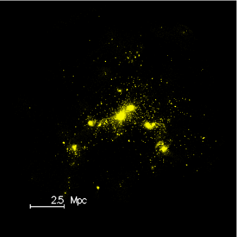
Figure 4: View of the third zoom level of the simulation (continued): stars.

Deriving merger trees from $N$-body simulations is not an easy task, because there is still a lot of freedom in defining halo and subhalo masses, and identifying both progenitors and sons in merger trees. There are two essential steps building merger trees: detecting the structures, and linking them from one timestep to the other. A “bad” structure detection results into a bad definition of the detected structures, and makes it impossible to extract results.

We used here the AdaptaHOP algorithm, and we followed the rules of T09 defining the haloes and subhaloes hierarchy as well as the merger history.

In addition, since we aim to study galaxies, we wish to detect separately the baryonic components, namely the central galaxies and their satellites.

3.1 Structure detection

Structure finders are widely used in computational cosmology to analyse simulations. Structure finders of the first generation, such as the FOF algorithm (Davis et al. 1985), were able to detect virialised DM haloes in the simulations.

The FOF algorithm links together particles closer than $b_{\text{link}}$ times the mean interparticle distance. It is efficient in finding haloes, but tends to link together separate objects when they are too close to each other, especially during mergers.

Spherical overdensities (SO, Lacey & Cole 1994) follows another approach: it detects density maxima, and grows from each maximum a sphere such that the mean density within this sphere is equal to a given value, e.g. $\Delta_{c}\times\rho_{c}$, where $\Delta_{c}\simeq 200$ (slightly depending on the cosmology and the redshift) is the virial overdensity, and $\rho_{c}$ is the critical density of the universe.

Denmax (Gelb & Bertschinger 1994), Bound Density Maximum (BDM, Klypin et al. 1999) and SKID (Stadel 2001) compute the density field, and move particles along the density gradients to find local maxima. Denmax computes the density on a grid, while in SKID the density field and its gradient are computed in a SPH way. Unbound particles are then iteratively removed via an unbinding step. HOP (Eisenstein & Hut 1998) has a similar spirit, but instead of computing density gradients, it jumps from one particle to its denstest neighbour, thus efficiently indentifies local density maxima. SUBFIND (Springel et al. 2001) finds subhaloes within FOF haloes by identifying saddle points. The density is computed in a SPH fashion. Each particle has a list of its two densest neighbours. Particles without denser neighbours are density maxima, thus correspond to a new substructure. Substructures then grow towards lower density particles. Saddle points are defined as particles that have their two densest neighbours belonging to two different substructures. AdaptaHOP (Aubert et al. 2004) is close to SUBFIND, except that the construction of the substructures occurs in a bottom-up manner, as we will later describe. Amiga’s Halo finder (AHF, Knollmann & Knebe 2009) is quite similar, but computes the density on an adaptive mesh refinement (AMR) grid, taking advantage of the adaptive nature of the AMR. VOBOZ (Neyrinck et al. 2005) is again similar, but uses a Voronoi tessellation to estimate the density. PBS (Kim & Park 2006) uses a total boundness criterion combined with a tidal radius to define substructures within FOF haloes.

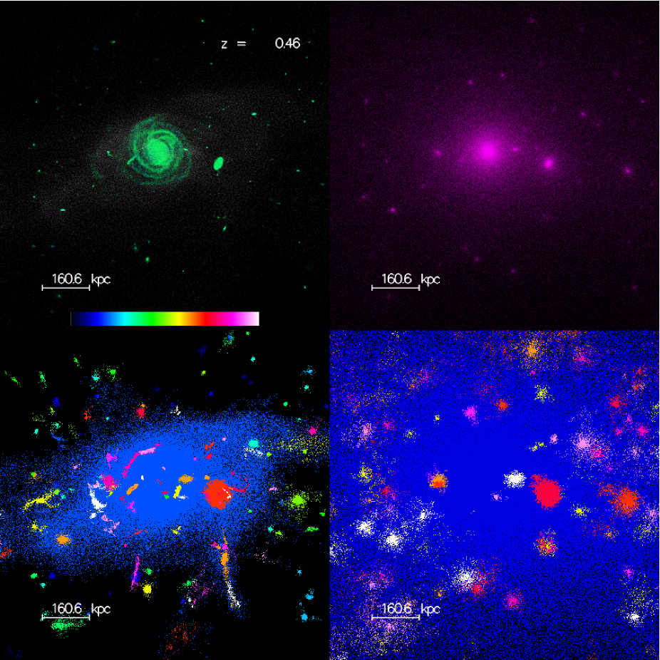
Figure 5: Zoom on the most massive halo of the third level of zoom. Same legend as figure 3.

All those algorithms are however only 3D, and based on the position of the particles. Several algorithms take advantage of the availability of the velocit data in addition to the positions. Six-dimensional (6D) FOF (Diemand et al. 2006) is a FOF algorthm with a 6D metric. Hierarchical structure finder (Maciejewski et al. 2009b) works in a similar way to SUBFIND in 6D, using a 6D density estimator. Rockstar (Behroozi et al. 2011) uses a 6D metric with the addition of time information

For a recent and more detailed comparative study of halo finders, we refer to Knebe et al. (2011). The structure finder must be applied to every snapshot of the simulation in order to build a merger tree.

We used AdaptaHOP to detect both DM and baryonic structures in the simulation. AdaptaHOP proceeds in four steps:

• First,the SPH density of particles is computed over $N_{\text{ngb}}$ neighbours. We chose $N_{\text{ngb}}=32$.

• Then, all particles whith density higher than the user-defined threshold density $\rho_{\text{T}}$ are selected, and the algorithm then jumps (“hop”) to their densest neighbour, thus finds the local maximum they belong to. A tree of structures is then built, the leaves of the tree corresponding to particles belonging to the same local maximum.

• Finally, the saddle points that link together two structures are identified.

• The algorithm then reiterates within each leaf of the structure tree to detect substructures.

The result is a tree of structures and substructures, where the leaves correspond to physical structures. The main parameters of AdaptaHOP are:

• $N_{\text{members}}$: minimal number of particles for a (sub)structure to be considered. It gives the minimal mass for a (sub)structure.

• $\rho_{\text{T}}$:density threshold of the first level, which is used to detect main haloes. Particles with a SPH density below $\rho_{\text{T}}$ are part of the background.

• $\alpha$: peak of the substructure. Only substructures with a density maximum $\rho_{\text{max}}>\alpha\bar{\rho}_{\text{sub}}$ are considered significant.

• $f_{\text{p}}$: Poisson noise parameter. The existence of a substructure is tested by comparing its density wih the Poisson noise: a substructure with $\bar{\rho}_{\text{sub}}>\rho_{\text{s}}\left(1+\frac{f_{\text{p}}}{\sqrt{N}}\right)$ is statistically significant, where $\rho_{\text{s}}$ is the density of the saddle point that separates the substructure from others, $\bar{\rho}_{\text{sub}}$ the mean density of the substructure, and $N$ the number of particles belonging to the substructure.

• $f_{\varepsilon}$: controls the size of the structure. Every structure must have a radius larger than $f_{\varepsilon}$ times the mean interparticle distance.

Following K05, we set $N_{\text{members}}=64$, which yields a minimum mass of $\simeq 8.96\times 10^{9}$ $\mathrm{M}_{\odot}$ for theDM haloes, and $1.92\times 10^{9}$ $\mathrm{M}_{\odot}$ for baryonic structures.

We note that we had to slightly modify the algorithm to make it compatible with the multi-zoom technique. Since particles enter the box between successive timesteps, $\bar{\rho}_{\text{box}}$ is indeed not constant, as opposed to regular simulations, and the evolution of $\bar{\rho}_{\text{box}}(t)$ for the four levels of zoom is shown in figure 2. We thus compared the density to $\rho_{\text{T}}$ times the mean density in the level 0 zoom, since the mean density in higher levels is higher than the mean density of the universe. At the last output, the mean density in the third level of zoom that we analyse is about 14 times the cosmic density.

3.1.1 DM halo detection

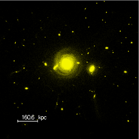
Figure 6: Zoom on the most massive halo of the third level of zoom (continued): stars.

Following Aubert et al. (2004) and T09, we defined haloes as groups of particles with densities higher than a given threshold density, and subhaloes as locally overdense groups of particles within a host (or main) halo, which separed by density saddle points. The centres of the haloes were defined as the positions of the densest particles in the halo rather than the centres of mass. The reason for this choice is that for a major merger, the centre of mass can be halfway between the two merging objects, and we preferred to define the “real centre” as the centre of the main halo.

In the following, the mass of a halo is defined as the mass of the main halo plus the mass of the subhaloes, therefore the mass of a subhalo can be counted several times.

As advocated in Eisenstein & Hut (1998), $\rho_{\text{T}}=80\times\bar{\rho}$, where $\bar{\rho}$ is the mean density of the universe (see previous section), was set for DM haloes, which is roughly equivalent to a linking length $b_{\text{link}}=0.2$ in FOF. We kept default values for the other parameters: $f_{\text{P}}=3,\alpha=1,f_{\varepsilon}=0.05$.

3.1.2 Galaxy detection

Several attempts have been made to build baryonic merger trees. Murante et al. (2007) used SKID (Stadel 2001) to detect baryonic structures, and they referred to as “family trees” the merger trees of baryonic galaxies, in order to avoid any confusion with subhaloes merger trees. However, they have only considerred star particles, whereas we also wish to take into account gas. Other authors have used SKID to detect both stars and cold gas, with $\rho/\bar{\rho}>1000$ and $T<3\times 10^{4}$ K (e.g. Simha et al. 2009).

Maller et al. (2006) also used SKID and introduced “virtual galaxies” in order to account for the fragmentation of baryonic structure between consecutive outputs. On the other hand, Dolag et al. (2009, 2010) used a modified version of SUBFIND to detect simultaneously dark matter and baryons, ending with a galaxy composed of DM, stars, and gas. They used dynamical criteria to distinguish between the central galaxy and the diffuse stellar component.

Our approach here was slightly different: we detected on the one hand the hierarchy of DM haloes and subhaloes, and on the other hand the baryonic component consisting of central galaxies and satellites.

We therefore also used AdaptaHOP to detect baryonic structures. While input parameters are known for DM detection, we had to find a more well-suited set of parameters in order to detect the baryonic structures. We set the density threshold $\rho_{\text{T}}$ above which structures are considered to 1000 times the mean (baryonic) density. We took $f_{p}=4$, $f_{\varepsilon}=5\times 10^{-4}$ in order to allow to detect structures with sizes of the order of 1 kpc, and kept $\alpha$ = 1. Higher values of $f_{p}$ tend to remove the smallest structures, while lower values add unphysical substructures.

3.1.3 Matching dark and baryonic structures

An interesting question that we addressed is how much baryonic matter there is in DM haloes. To answer this question, we studied the link between galaxies and haloes, taking advantage of their independent detections. We then set several rules to decide whether a galaxy and a halo are linked together.

The first rule is that a galaxy should belong to at most one (sub)halo (and of course its host halo hierarchy if it is a subhalo). The second rule is that the hierarchy of galaxies and satellites on the one hand and haloes and subhaloes on the other has to be respected, so that we avoid the case where a satellite is linked to the host halo while the galaxy is linked to the subhalo. With these rules, a halo $h$ can host several galaxies, but at most one main galaxy $g$, which is the most massive galaxy of $h$ and must have $h$ as its halo. Bearing these rules in mind, we were able to match DM haloes to galaxies.

3.2 Merger tree building

In the context of structure finding, one of the most persistent problems is the so-called flyby issue. This phenomenon can occur when two haloes cross each other, and when their respective centres are too close to each other. They are then detected as only one halo – even if they can sometimes still be distinguished by eye – and thus considered as a merger, but detected again as two separated haloes at a later timestep.

This problem can be partially resolved by using a subhalo finder such as AdaptaHOP instead of a halo finder such as FOF, since the second halo can still be tracked as a subhalo, thus conserve its identity; however the problem remains when the subhalo is too close to the host halo centre. An improvement would be to use a phase-space halo finder, such as HSF (cf Maciejewski et al. 2009a, b). Sinha & Holley-Bockelmann (2012) introduced an interesting method called “halo interaction network”, which is a more complex merger tree that takes into account flybies. However, for this work we were only interested in discriminating between particles entering smoothly from the background and particles belonging to another structure and entering by means of mergers, hence we did not need such a refinement.

Tweed et al. (2009) give different sets of rules building DM merger trees that include subhaloes, where a (sub)halo at output $t_{n+1}$ is the son of its progenitor at output $t_{n}$. We refer to a structure as either a subhalo or a halo. These rules are:

• A structure can have at most one son.

• The son of structure $i$ at output $t_{n}$ is the structure $j$ at output $t_{n+1}$, which inherits most of the mass of structure $i$.

• Structure $i$ at output $t_{n}$ is a progenitor of structure $j$ at output $t_{n+1}$, if $j$ is the son of $i$.

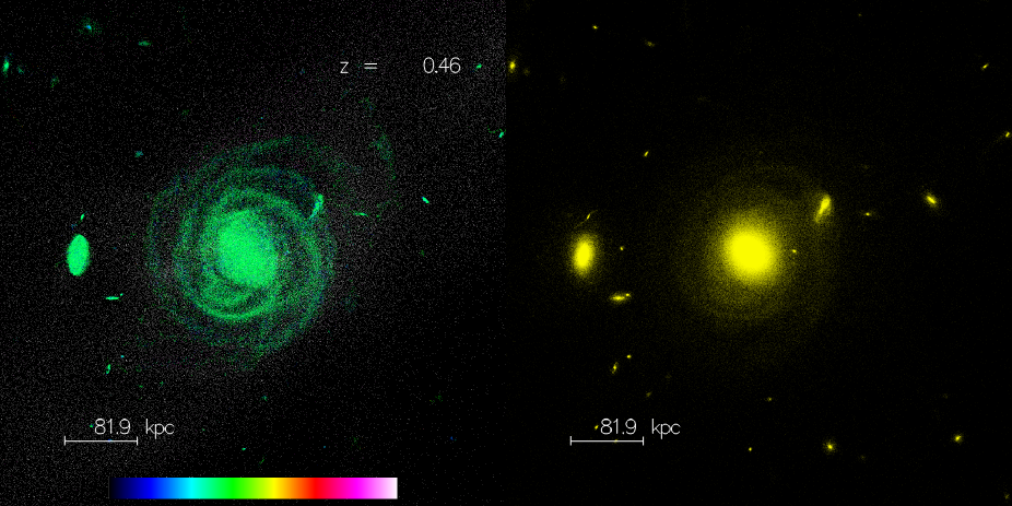
(a) face on

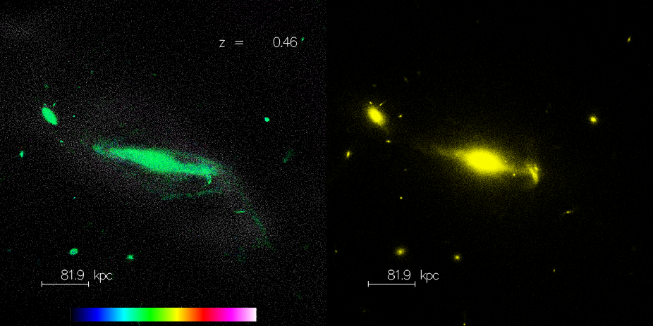
(b) edge on

Figure 7: View of the most massive central galaxy, at $t=9.1$ Gyr, in the third level of zoom. Left: gas colour-coded by temperature from 800 to $1.4\times 10^{6}\,\text{K}$, right: stars.

They introduced a two-step method called the branch history method (BHM) to determine which of two local maxima should be the subhalo and which the main halo, according to the results of the previous step.

This method tends to avoid identity switches between the main halo and the satellite. The basic idea is to take advantage of the previous snapshot to decide which node should be the subhalo and which the halo.

Once again, we had to modify the algorithm to take into account the number of particles, which is not constant with time owing to our use of the multi-zoom method.

3.3 Accretion history

After we had built the full merger tree of each galaxy, we were able to compute the mass history. We traced back the main progenitor from the last snapshot to the first, and tagged each particle entering the main structure at each snapshot. Particles coming from either a satellite of the considered galaxy or from another galaxy were tagged as merger, while particles coming from the background were defined as smooth accretion.

Particles can also leave the main galaxy, either for the background, which we refer to evaporation, of for another substructure, which we dub fragmentation. The latter happens mainly during mergers events: particles from a satellite are detected as part of the main galaxy at a given snapshot, but may have left before the following. The former can happen at almost every snapshot: for particles at the border of the structure, density can fluctuate without moving, thus be on either one side of the saddle point or the other.

With these definitions, we were able to compute the baryonic mass assembly: merger $-$ fragmentation and accretion $-$ evaporation. The mass of a structure was counted only once, since a particle entering the galaxy is counted positively, and negatively when it leaves. This enables us to overcome the fly-by issue mentioned above, since a fly-by would be counted first as a merger, then as fragmentation and could then vanish in the total accretion fraction.

However, there is another difficulty: as a consequence of the multi-zoom technique, particles enter a higher zoom-level box at each timestep, thus several galaxies enter the box when they have already formed. Accretion fractions are computed between $t_{\text{app}}$, the time when the galaxy enters the last zoom level box, and $t_{\text{end}}$, the end of the simulation. We thus concentrated on galaxies entering the box before $t=7$ Gyr in order to follow them over a sufficient number of timesteps.

4 Results

4.1 Structure detection and merger trees

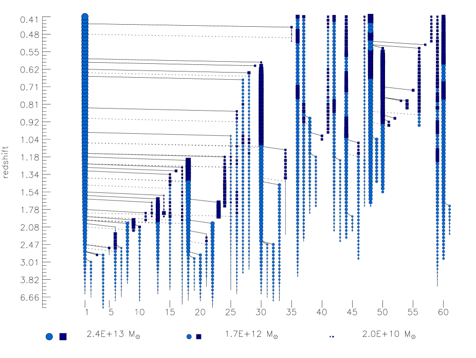
Figure 8: Baryonic merger tree of the main galaxy. Dark blue circles are galaxies, and bright blue squares satellites. The $x$ axis shows the number of the branch, i.e. a galaxy that will eventually merge with the main galaxy (branch 1), or stay as one of its satellites.

Figures 3 and 5 show, respectively, a large-scale view of the third level of zoom of the simulation and a zoom on the most massive galaxy of the box. The upper panel shows on the left gas particles (colour-coded by temperature, on a logarithmic scale from 800 K to $1.4\times 10^{6}$ K), and on the right, DM particles. Figures 4 and 6 show the corresponding star distributions.

The lower panel shows the structures detected by AdaptaHOP, baryonic galaxies and satellites on the left, and DM haloes and subhaloes on the right. Haloes and main galaxies appear in dark and light blue and green, and subhaloes and satellites appear in yellow, orange, red, magenta, and white. At the centre, the most massive halo (in blue) can be seen with massive subhaloes (in magenta and white): it is undergoing a major merger at this timestep, which explains why these massive substructures appear larger than several small and isolated haloes.

We can see by eye the good agreement between the baryonic and DM structure detected. However, since for a given galaxy the DM halo is far more extended than the baryonic structure, this is not easy. In section 3.1.3, we explained how we matched galaxies and haloes.

The zoom in figure 5 is instructive. We can still discern the close correspondence between the dark and baryonic structures, and most of the small structures in the upper panels are indeed detected in the lower panels. However, some remarkable features can be found: in the bottom left panel, there is a satellite (in orange, under the largest satellite in yellow) with a tidal tail (in red), which is detected by AdaptaHOP as a satellite whose tail is a “satellite” of this satellite. This structure finder is thus capable of detecting interesting features.

Most strikingly, the red arc near the centre of the main galaxy is an artefact: it is not a satellite, but rather an arm of the spiral galaxy.

In figure 5, we can see the central galaxy of the halo, which contains a large disc of $\simeq 160$ kpc (comoving) at $z=0.46$. Figures 7(a) and 7(b) show, respectively, a face-on and an edge-on view of the central galaxy. Looking at the corresponding galaxy at $z=0$ in our level 2 simulation, it appears that this galaxy still has a gaseous and stellar disc today, which is quite unexpected since central galaxies are supposed to be elliptical. The large size and mass ($\simeq 10^{13}\,\mathrm{M}_{\odot}$) of the galaxy is probably caused by our not taking into account AGN feedback in our simulations.

Figure 8 shows the merger tree of this galaxy. Only the 60 most massive branches of the tree are shown here. The $y$ axis is the redshift, and each branch is a galaxy that either completely merges with the main galaxy, or becomes a satellite of this galaxy at the last timestep. The first branch on the left is the main progenitor branch, i.e. the ancestors of the main galaxy. Branches 2 to 35 are galaxies (bright blue circles) that became satellites (dark blue square) of the main galaxy, and merged with it before the last timestep. Branches 36 to 61 are the satellites of the main galaxy at the last timestep, and their merger trees.

Galaxies that seem to appear in the merger tree at low redshift are actually entering the level 3 zoom at this time (e.g. branches 42–51). However, satellites that seem to appear late (e.g. branches 23, 24, 42) correspond to fly-bies: they have no identifiable progenitor at any previous timestep.

4.2 Evolution of the mass function

Since we built the merger trees of all galaxies and dark matter haloes, we were able to study the evolution of the mass function with time. Figure 9(a) and 9(b) show, respectively, the cumulative distribution of mass of baryonic galaxies and DM haloes at three timesteps of the simulation, the three curves (blue, green, and red) corresponding to $t=3,6,$ and 9 Gyr, respectively (or $z=2.23,1.02,$ and 0.47), in our third level of zoom. We computed the mass of structures and substructures therein, counting the mass of substructures several times: once as stand-alone substructures, and then as part of their host structures. The evolution of the mass function is compatible with a hierarchical growth of structures, with fewer massive structures, both in galaxies and DM haloes, existing at higher redshift than at lower, and with a slope that flattens towards lower redshifts. However, it must be emphasised here that the resulting mass functions are biased we ahve zoomed into an overdense region. These results could however be compared to Crain et al. (2009), who performed resimulations of several regions of the Millennium simulations.

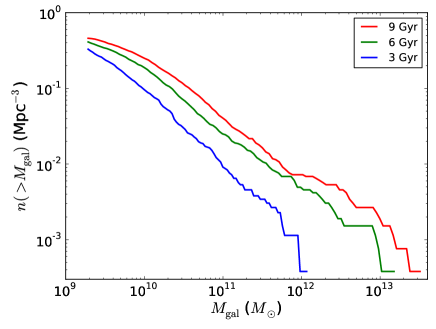
(a) Galaxies

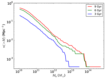
(b) Haloes

Figure 9: Cumulative mass distribution of galaxies and satellites (left) and haloes and subhaloes (right) at the third level of zoom, at $t=3$ Gyr (blue), $t=6$ Gyr (green), and $t=9$ Gyr (red) ($z=2.29,1.02,$ and 0.47).

To compare several structure-finding codes, we performed another structure detection with FOF, using a linking length of $b=0.2$ times the mean interparticular distance. Figures 10 shows the halo mass function at the four zoom levels, respectively, for FOF (dashed line) and AdaptaHOP (solid line) haloes. This time we note that the subhaloes are not counted separately, but are included within the AdaptaHOP haloes to permit us to compare them with FOF haloes. Level 3 is shown in green, level 2 in blue, level 1 in red, and level 0 in magenta. The black solid line is a Press and Schechter function, computed by the code described in Reed et al. (2007) for our adopted cosmology, and the dotted line the mass function from the Millennium simulation (Springel et al. 2005). The FOF and AdaptaHOP mass functions show differences, especially at low masses. Indeed, several small haloes that are detected by FOF and located close to the edges of a larger FOF halo are detected by AdaptaHOP as substructures of this halo, thus they do not appear as low mass structures in the AdaptaHOP curve. However, at higher masses there is a good agreement between the two structure finders. Only the level 0 (cosmological run) mass function can be directly compared with the theoretical predictions of Press & Schechter and with the Millennium mass function, although it is instructive to overplot the mass functions for the three other simulations. The comparison with the Press and Schechter mass function can be seen as a probe of our environment and a way to quantify the overdensity. Our mass function agrees with both the Millennium and the Press & Schechter mass functions. The mass functions in the other zoom levels show the density of the environment with respect to the cosmic average.

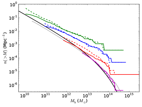
Figure 10: AdaptaHOP (solid line) and FOF (dashed line) halo mass function for the four zoom level: level 3 in green, 2 in blue, 1 in red, and 0 in magenta. Note that subhaloes are not counted separately, but are included within the AdaptaHOP haloes in order to compare with FOF haloes. The black line is a Press & Schechter predicted mass function, for the sake of comparison, and characterisation of the environment.

4.3 Baryonic fraction

According to WMAP data (Komatsu et al. 2011), baryons represent about 4% of the Universe content, yet only a small fraction are seen. One can legitimately ask where the baryons are in the Universe. We computed the baryonic fraction, i.e. the ratio of the baryonic mass to the DM mass, for each halo in the simulation, at several timesteps. We defined the halo centre as the position of the densest particle, and the radius of a (sub)halo as the distance between the centre and the furthest-away particle. For each halo or subhalo detected, we computed the total baryonic mass within and plotted the baryonic fraction $m_{\text{b}}/m_{\text{halo}}$ as a function of the (sub)halo (including all its subhaloes) mass, as discussed in § 4.2. For each baryonic particle, we computed its closest dark matter particle, and assigned the baryonic particle to the halo of its corresponding DM particle. This method enabled us to consider any geometry of halo. Haloes undergoing major mergers, which is the case for our largest halo, may indeed have a non-spherical shape.

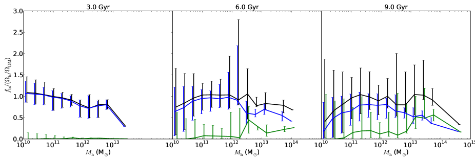
Figure 11: Median of the baryonic fraction computed in logarithmic bins as a function of the halo mass in the level 3 zoom at $t=3,6,$ and $9.0$ Gyr, normalised by the universal fraction $\frac{\Omega_{\text{b}}}{\Omega_{\text{DM}}}$. The total baryonic fraction is shown in black, the stellar fraction in green, and the gas fraction in blue. The errorbars represent the 85^th and 15^th percentiles.

The baryon fraction, or the ratio of stellar mass to dark mass as a function of time and galaxy mass can be compared with that expected based on analyses of observations with the halo abundance matching technique (HAM). This tool was developped by Vale & Ostriker (2004) and has been used by several groups. Assuming that there is a tight correspondence between the stellar masses of galaxies and the masses of their host haloes, and matching their number density or abundance, this technique allows to deduce average relations linking the baryon and dark matter growths over time, given that the observed galaxy stellar-mass function, and its variation with redshift, is satisfied as input. Conroy & Wechsler (2009) show for instance that the stellar mass growth is essentially due to both accretion and star formation, while the merger process has little influence and most massive galaxies must form their stars earlier than less massive ones (downsizing). The stellar mass fraction with respect to the universal baryon fraction reaches a maximum of 20% in haloes that have a virial mass of a few 10¹² M_⊙ at $z=2$, and the maximum is reached at lower halo mass with time, down to a few $10^{12}\,\mathrm{M}_{\odot}$ at $z=0$. Figure 11 shows the median of the baryon fraction (in black), stellar fraction (green), and gas fraction (blue) computed in logarithmic mass bins, at $t=3,6,\text{and }9$ Gyr, and such an evolution can be seen, with a peak in the stellar fraction at $\simeq 10^{12}\,\mathrm{M}_{\odot}$, which is compatible with Conroy & Wechsler (2009). These values are to some extent compatible with the relation found by Behroozi et al. (2010), who consider in more detail the uncertainties and scatter caused by various assumptions. However, unlike these authors, we still have a higher stellar fraction at higher than at lower mass. This can be atribudet to our neglect of feedback from AGN in our simulations, which is thought to be responsible for preventing star formation in massive haloes. Observations of galaxies in groups and clusters (e.g. Hoekstra et al. 2005; Dai et al. 2010) also show that there is a drop of the stellar fraction towards high masses.

Interestingly, this plateau at high masses is compatible with the simple prescription in Nipoti et al. (2012), for which the stellar-to-halo mass relation is modelled by a power law.

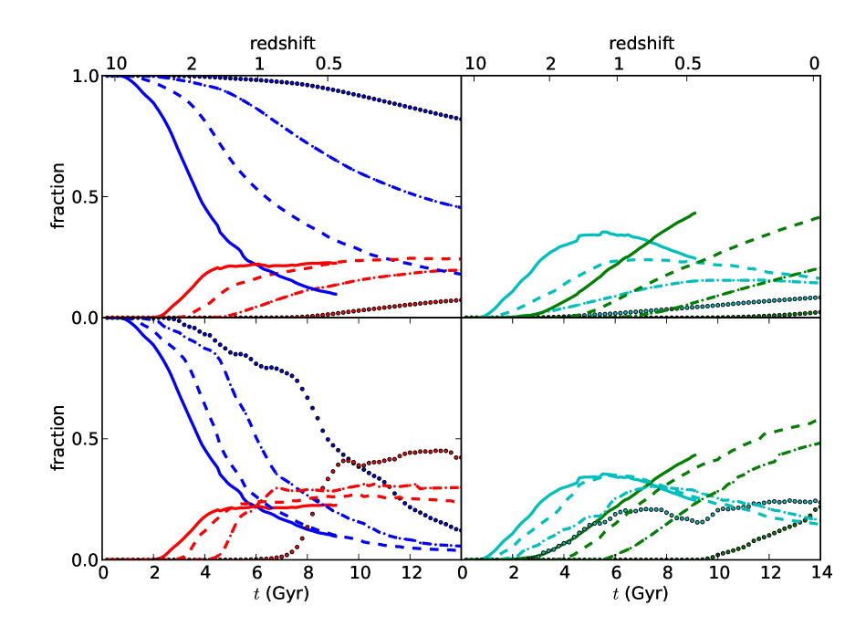
Figure 12: Baryon fraction in four phases: diffuse gas (blue), condensed gas (cyan), hot and warm-hot (red) and stars (green), at level 3 (solid), 2 (dashed), 1 (dash-dotted), and 0 (dotted). In the top panels, the fraction is computed in the full box of each level, and in the bottom panels, it is computed only within the 8.56 Mpc radius of the level 3 box. The differences are then only caused by those in the resolution.

We studied the relative fraction of baryons in different phases, following Davé et al. (2001). We distinguish between four phases according to the gas temperature and density contrast $\delta=\rho/\bar{\rho}-1$.

• Diffuse gas: $\delta<10^{3}$, $T<10^{5}$ K.

• Condensed gas: $\delta>10^{3}$, $T<10^{5}$ K.

• Hot and warm-hot: $T>10^{5}$ K.

• Stars.

The evolution of each phase for the four levels of zoom is plotted in Fig. 12. Top panels show the hot/warm-hot (red), diffuse (blue) gas, condensed gas (cyan), and stars (green), computed for the four levels of zoom. These four levels have a similar trend of diffuse gas that condenses and forms stars as cosmic structures evolve, and the fraction of hot and warm-hot gas that increases when there are massive enough structures to heat the gas, before eventually reaching a plateau. It is worth noting that the condensed gas fraction reaches a maximum at $z\simeq 2$, which corresponds to the peak of the cosmic star-formation rate (e.g., Bouwens et al. 2010).

However, the condensation rate changes from one zoom level to the other. The difference between the four levels of zoom may be due to either the resolution or the environment: level 0 is indeed a cosmological box whereas level 3 is centred on a dense region, and we expect to obtain different results owing to the different environments. To distinguish both effects, we plotted in the bottom panels the same fraction, but computed for each level only within the 8.56 Mpc spherical box of level 3. This time, the difference between the different zoom levels are due only to the resolution. We can see that there is a good convergence between levels 2 and 3.

4.4 Dark and orphan galaxies

Since we were able to match galaxies to haloes, we checked whether there was any “dark galaxy”, halo without any baryonic counterpart, or “orphan galaxy”, galaxy without a dark matter halo.

We were unable to detect any orphan galaxy: all galaxies in the simulation lie within a halo. However, not all galaxies are the main galaxy of either a halo or subhalo. We defined galaxies as the main structures identified with AdaptaHOP for baryonic particles, and satellites to be their substructures. These definitions differ from those usually assumed, where central galaxies are at the centre of a halo, and all other galaxies are satellites. Therefore, several detected structures that we classified as “galaxies” would be called “satellites” by other authors. Several of them are close to the halo centre, and cannot be associated with a resolved subhalo. Whether this is due to a lack of resolution or to physical subhalo stripping is still unclear.

We detected several “dark galaxies” without any baryonic counterpart, about 100 haloes and 100 subhaloes at $t=9$ Gyr. They are represented in figure 11 in cyan (haloes) and magenta (subhaloes). We investigated whether they contained any baryons and found that they appear to contain few gas particles. When looking at these dark haloes and subhaloes, it appears that most of the dark haloes have gas, but that these structures are insufficiently well-resolved hence not dense enough to form stars and be detected as a galaxy. We therefore checked that these dark haloes and several subhaloes are also detected by FOF, and are not spurious detections by the halo finder. Most of the dark AdaptaHOP haloes were also detected by FOF, and one can believe that they are of a physical significance. They often contain clouds of gas that are not dense enough to be detected as galaxies, which could be an effect caused by a too low resolution. Some dark subhaloes were also detected as FOF haloes, most of them however appear to be non-physical structures, for example bridges between two real subhaloes containing a galaxy.

By varying the sets of parameters in AdaptaHOP, we found different numbers of dark galaxies. This is because these haloes are very close to the detection threshold, and are detected as haloes or subhaloes for a given set of parameters, while they are undetected for a less conservative set.

4.5 Velocity dispersion

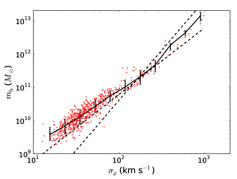
(a) Galaxies

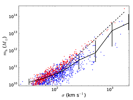
(b) Haloes

Figure 13: Mass versus velocity dispersion . Left: galaxies; right: haloes(red) and subhaloes (blue). The solid black line is the median of the baryonic (stellar plus gas) mass of galaxies (panel 13(a)) and dark matter mass of haloes and subhaloes (panel 13(b)) and the errorbars are the 15^th and 85^th percentiles. The dashed black line in the right panel shows the expected slope $m\propto\sigma^{3}$, and on the right panel, the lines show the slopes $m\propto\sigma^{3}$ and $m\propto\sigma^{2}$.

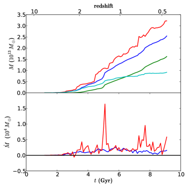
(a) Galaxy 2

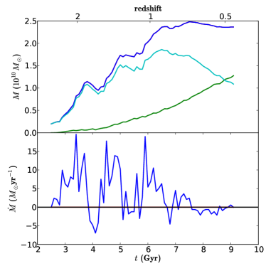
(b) Galaxy 56

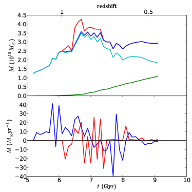
(c) Galaxy 469

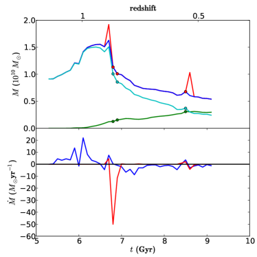
(d) Galaxy 512

Figure 14: Top: Mass history of four typical galaxies. Blue curves: baryonic mass of the galaxy. Red curves: baryonic mass of the galaxy plus its satellites. Green curve: stellar mass of the main galaxy. Cyan: gas mass. Bottom: Mass origin, where red represents a merger from another (sub)structure and blue, smooth accretion from the background.

We computed for each substructure, baryonic and (sub)halo and galaxy the velocity dispersion $\sigma_{v}$ at several snapshots. Since AdaptaHOP does not perform an unbinding step, some particles that are spatially close to a structure can be attached to the latter, although they are not dynamically bound. To get rid of the contamination of these particles, special care has to be taken. We used a two-step algorithm. First, we defined the bulk velocity of the structure by computing the median of each component of the velocity, which is more robust than taking the mean value because high velocity particles have a weaker influence on the median. We then selected only particles with a velocity close enough to the bulk velocity. To do so, we computed the circular velocity at the half-mass radius, i.e. the radius containing half the mass of the structure, $v^{*}=\sqrt{\frac{GM(<r_{\text{half}})}{r_{\text{half}}}}$, which gives a characteristic velocity for the structure. The velocity dispersion was then computed for particles whose velocity relative to $\@vec{v}_{\text{bulk}}$ is lower than $nv^{*}$. These are the most bound particles. We checked that our result does not strongly depend on the choice of $n$, and took $n=5$.

With this technique, only one halo and seven subhaloes could not be treated because no particle was selected. We checked that these structures corresponded to unbound structures and dropped them from our analysis.

We computed the 3D velocity dispersion for dark matter (sub)haloes. To compare our results for baryonic galaxies and satellites with obsevations, we defined the velocity dispersion as follows: for massive galaxies ($M>10^{11}$ $\mathrm{M}_{\odot}$), we computed the dispersion in the projected stellar velocity in radial bins along the $x$ axis, and defined the velocity dispersion of the structure as the value in the bin containing the half-mass radius. For lower mass galaxies, which are less well-resolved, the velocity dispersion is computed over all stellar particles.

In this section, the mass of the structures does not take into account the substructures, since we do not wish to account for the velocity dispersion of particles within the substructures.

Figure 13 shows the velocity dispersion as a function of the mass for galaxies in panel 13(a) and DM haloes (red) and subhaloes (blue) in panel 13(b).

The dashed black line in the right pannel shows the expected slope $m\propto\sigma^{3}$, and on the right pannel, the lines show the slopes $m\propto\sigma^{3}$ and $m\propto\sigma^{2}$.

The relation between mass and velocity dispersion for dark matter haloes is compatible with a power law with the expected slope of three, although our data suggest a slightly shallower slope. Observations indicate that there is a tight correlation between the total baryonic mass of galaxies and $V_{\text{max}}$, the maximum of the velocity curve, which is referred to as the baryonic Tully-Fisher relation (BTRF). However the observed exponent is close to four (eg McGaugh et al. 2000; Courteau et al. 2007; McGaugh 2012). In our case, the slope agrees with the BTRF at high masses, but at low masses it is lower than expected.

5 Accretion and merger history

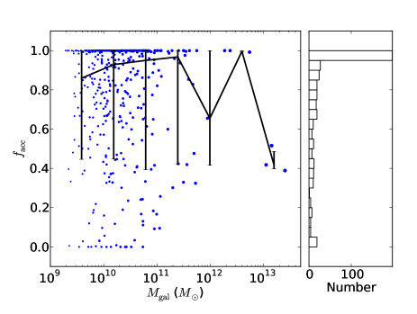
Figure 15: Accretion fraction versus galaxy mass, and the associated histogram (in number), computed for the 530 galaxies entering the box before 7 Gyr. The size of the markers is proportional to the logarithm of the galaxy mass. In the right panel, red dots correspond to galaxies that are outside the level 3 box. The black line show the median of the accretion fraction, and the errorbars the 15^th and 85^th percentiles. We find a mean accretion fraction of 77%.

The upper panels of figure 14 shows the mass history of four characteristic galaxies of the simulation: a massive galaxy both accreting gas and growing by mergers, a small galaxy growing only through accretion, a galaxy growing by means of bowth mergers and fragmentation, and a galaxy losing mass by means of fragmentation while passing a larger galaxy. The blue curve is the baryonic mass of the galaxy itself, while the red curve shows the mass of the galaxy plus its satellites. The stellar mass is plotted in green, and the gas mass in cyan. A galaxy may be detected as a satellite of another galaxy during its history. These timesteps are plotted as circles (panel 14(d)).

The bottom panels of figure 14 show the origins of the mass, separated into two components: merger and accretion. Smooth accretion is shown in blue and mergers in red. A negative value of merger or accretion, respectively, means that the galaxy loses mass to either another galaxy (fragmentation) or the background (evaporation). These are the two components of the derivative of the blue curve shown in the upper panel, since with our definition, all mass is acquired by either merger or smooth accretion, and lost by fragmentation or evaporation.

Those four galaxies have very different mass accretion histories. The galaxy in panel 14(a) undergoes a major merger that can be seen in the lower panel of 14(a), at $t\simeq 5.1$ Gyr.

The galaxy in panel 14(b) shows the opposite behaviour: it does not experience any merger and grows smoothly by accreting gas until $t\simeq 7$ Gyr, then maintains a constant mass until the end of the simulation, passively turning its gas reservoir into stars.

In panel 14(c), the galaxy grows mainly through accretion until it reaches a maximum mass at $t\simeq 7$ Gyr, and then interacts with another structure and loses more mass than it gains from mergers, and ends with a somewhat lower mass.

Galaxy in panel 14(d) shows quite an unusual behaviour: after entering the level 3 box at $t\simeq 5\text{ Gyr}$, it grows from both mergers and accretion, and is suddenly accreted by a more massive galaxy, becomes a satellite, then loses about one third of its mass, which feeds the host galaxy. It then leaves its host galaxy and continues to lose mass through evaporation. These behaviours are quite typical of what we can see in our simulations, with high-mass central galaxies undergoing mergers and accreting, and lower-mass, isolated galaxies accreting gas before their growth is stopped.

We computed the accretion fraction by considering, at the last output, the origin of each particle: particles belonging to the galaxy at the first time of detection were defined as “initial”; particles that came originally from the background, and had never belonged to another structure were labelled “accretion”; and we defined as “merger” a particle that had been accreted into the main progenitor of the galaxy and previously belonged to another structure, even if it is coming from the background. We defined the accretion fraction as

$$f_{\text{acc}}=\frac{\text{accretion}}{\text{accretion + merger}},$$ (3)

and the merger fraction $f_{\text{merg}}$ such that $f_{\text{acc}}+f_{\text{merg}}=1$. By definition, we have $0\leq f_{\text{acc}},f_{\text{merg}}\leq 1$.

As a consequence of the multi-zoom thechnique, and that galaxies can enter the level 3 box during the simulation, we had to select galaxies to be studied. We only computed this accretion fraction for galaxies that could be tracked back in time until before $t=7$ Gyr so that the fraction could be computed for at least 2 Gyr of its lifetime. We discarded galaxies that could not be tracked earlier than 7 Gyr, which either entered the box later, or were lost when computing the merger tree, possibly after a merger event. This left us with 530 galaxies that had been tracked from $t_{\text{app}}<7.0$ Gyr to $t=9.1$ Gyr.

Figure 15 shows the accretion fraction as a function of mass for these 530 galaxies, as well as the (number) histogram of the accretion fraction. We found a mean accretion fraction of 77%, and a median value of 92%. In black, we plotted the median accretion fraction in mass bins, where the errorbars are the 15^th and 85^th percentiles. We can see that most galaxies have a very high accretion fraction. The trend for low-mass galaxies at $f_{\text{acc}}=1$ indicates that several galaxies undergo no mergers and are fed only by accretion. This could be a spurious effect caused by galaxies entering the box at late time, and experiencing no mergers. However, even when we consider only galaxies that are present in the box between 3 Gyr and 9.1 Gyr, the histogram still shows such a trend with a mean value of 70% and median of 82%. The four points in the upper right region are particularly striking: they correspond to massive galaxies that would have acquired their mass mostly smoothly. When sudying the details, they correspond to galaxies that entered the level 3 box a few snapshots before our limit of 7 Gyr, and have experienced no merger since this date, hence have a high accretionfraction. However, they are likely to have undergone mergers before entering the level 3 box.

6 Downsizing

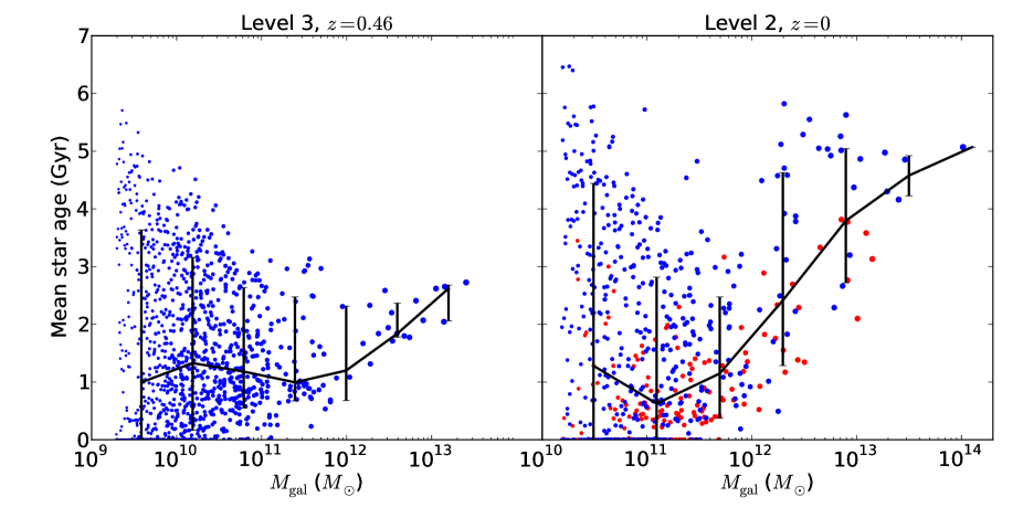
Figure 16: Median of the mean stellar age of the galaxies as a function of the galaxy mass at the last output for level 3 ($z=0.46$) and 2 ($z=0$). The markersize is proportional to the logarithm of the mass. In the right panel, the blue points correspond to galaxies within the $R_{3}=8.56$ Mpc of the third level of zoom, and the red points to galaxies outside this region. The errorbars show the 15^th and 85^th percentiles.

We now study the mean stellar age of galaxies as a function of the galaxy mass. For this study, we use both zoom levels two and three because the level three simulation stops before $z=0$, but has a higher mass resolution. Figure 16 shows the median of the mean stellar age of the galaxies as a function of the galaxy mass at the last output for level 3 ($z=0.46$) and 2 ($z=0$). The errorbars correspond to the 15^th and 85^th percentiles.

The differences between the blue dots in the two panels are then due bowth to our low resolution and the temporal evolution. It is interesting to see that in the second level of zoom, galaxies outside the $R_{3}=8.56$ Mpc radius (i.e., red points) formed their stars more recently than the ones within the box (blue points). This is certainly due to the lower average density of the region in the level 2 simulation which is located outside of the level 3 box. We can see that at low masses, the dispersion is large: among the least massive galaxies, some form their stars early, while others form them late. At each epoch of the universe, there is a large number of dwarfs, whose stars are forming actively. This behaviour is not seen for massive galaxies. The scatter in the stellar age progressively reduces with time, as mass increases. The most massive galaxies form their stars at a precise epoch, 7-8 Gyr, which correspond to half the universe age, depending slightly on the level of resolution. After this epoch, their star formation drops considerably, which may be due to environmental effects that suppress the cold gas reservoirs.

This behaviour is compatible with both hierarchical structure formation, since low-mass galaxies are the first to form and then be involved in the formation of more massive galaxies, and the observed downsizing, since the most massive galaxies are not observed to form stars at $z=0$, but have formed most their stars when the universe was half of its present age. Today, star formation continues only in small galaxies, although it was also the case in the early universe.

7 Discussion

7.1 Influence of the resolution

An important question is how variation in the numerical resolution influences our results. Our study of the baryon phase evolution in figure 12 provides a first evidence of numerical convergence, especially between levels 2 and 3. To study the consistency in greater detail, we compared the mass assembly history of several galaxies at zoom levels 2 and 3. We identified these galaxies in those two levels of simulations, and applying the same algorithms we compared their history. Since the mass threshold is the same, 64 particles, we expect that in the level 2 zoom, fewer satellites are detected and sub-resolution mergers play a role, thus the accretion fraction should be larger.

There are some galaxies for which the evolution is far from complete at $t=9$ Gyr. We take the example of galaxy 1 in figure 14(a). Figure 17 shows its mass assembly, the plain line is level 3 and the dashed line level 2. We can see that the mass of the galaxy is almost similar in the two zoom levels, but the mass of the satellites is lower in the level 2 zoom.

However, in the level 2 zoom, the galaxy is first detected at $t=2.8$ Gyr, whereas in the level 3 one, it is detected at $t=1.2$ Gyr, owing to a lack of resolution at level 2.

We found that the accretion fraction between $t=0$ and $t=9.0$ Gyr is 0.64 at level 3 and 0.81 at level 2. However, since level 2 reached $z=0$, we were able to compute the accretion fraction for the entire formation history of the galaxy. We found that $f_{\text{acc}}=0.53$, which is lower than the accretion fraction computed until $t=9.0$ Gyr. This is because this galaxy undergoes major mergers at $t\simeq 12$ Gyr as we can see in figure 17. We also computed the formation time $t_{\text{form}}=11.6$ Gyr, i.e. the time at which the galaxy assembled half of its mass at $z=0$, which we show as a vertical black line in the figure. For this galaxy, owing to the late major merger, $t_{\text{form}}$ is greater than 9.1 Gyr, which means that it has assembled less than half of its mass; however, most galaxies have a formation time that is lower than 9.1 Gyr.

7.2 Overcooling issue

As pointed out in section 2.2, no AGN feedback was included in this simulations serie. Active galactic nucleus feedback has been invoked to resolve the over-cooling problem in massive galaxies. This could be done in several ways, and the complete issue has not yet been definitely settled. At late times (low redshift), when large structures have formed, the so-called “radio mode”, coming from radio jets emitted by super-massive black-hole, is certainly efficient in preventing cooling flows (Croton et al. 2006; Bower et al. 2008), but theirefficiency is believed to be local, and the action of AGN at higher redshift, (or the quasar mode) even before the formation of groups and clusters, is thought to be more effective in preventing the over-cooling (e.g., McCarthy et al. 2011). Studies taking into account AGN feedback (e.g., Guo et al. 2011) obtain more realistic stellar masses for massive haloes.

Supernova feedback is efficient for low-mass haloes, where kinetic energy can be transferred into the gas, enabling it to escape the halo. However, the present simulation is focused on a massive cluster, where the escape velocity is so high that SNe feedback is insufficient to expel the gas from the halo. This results in the overcooling of baryons and eventually to very high stellar masses in our more massive haloes (about $10^{13}$ $\mathrm{M}_{\odot}$). We believe that, although some results might suffer from overcooling, our predictions should be robust at least for the range of lower mass galaxies. In a future paper, we will include various forms of AGN feedback and address how our main conclusions should be modified as a consequence.

7.3 Comparison with previous work

We found that galactic mass assembly is dominated by gas accretion rather than by mergers, even though we might be unable to detect mergers of low mass satellites. However, we do not expect them to add a significant contribution (Murali et al. 2002, K05). We note that we cover a comparable volume, with a comparable resolution to K05, although the main advantage of our simulation is that we are able to simulate a rich environment starting from a cosmological box.

Our results are in good agreement with SC05, who found a typical accretion fraction of 70%. We also appear to agree with Simha et al. (2009), who studied the mass growth of central and satellite galaxies. However, we do not have the same definition of central galaxies and satellites. They call a central galaxy the most massive galaxy at the centre of a FOF-halo, and all other galaxies lying in the halo or one of its subhaloes are called satellites. As a consequence, hey have “central” galaxies of subhaloes that are still accreting satellites, but with their definitions these galaxies are considered as satellites. Nickerson et al. (2011) studied the satellite loss mass in a SPH simulation of a Milky-Way type galaxy and its satellites through UV-ionisation, ram pressure stripping, stellar feedback, and tidal stripping. They found that tidal stripping reduces significantly the mass of bright satellites, which become of lower mass than some dark ones, and that stellar feedback mostly affects medium-mass satellites. van de Voort et al. (2011) performed a similar study using the Gadget-3 TreeSPH OWLS simulations. They computed the accretion rate onto both dark matter haloes and galaxies, and found that the cold accretion dominates the mass assembly. However, we note that we have not separated gas accretion into two different components, namely cold and hot accretion, and considered here only accretion as opposed to mergers. Faucher-Giguère et al. (2011) also found that the contribution of mergers to mass assembly is minor, and confined to high mass haloes. They studied in detail the fate of accreted gas, through cosmological hydrodynamical simulations. They confirmed that galaxies accrete mostly warm and hot gas above a critical halo mass of $3\times 10^{11}$ $\mathrm{M}_{\odot}$ at $z=0$ as proposed by Birnboim & Dekel (2003), and that the fraction of cold gas accretion increases with redshift. Their variation in the SNe feedback and efficiency of galactic winds demonstrated that this essentially unknown parameter can decouple the gas accretion from the star formation rate, and efficiently decrease the baryon fraction in low-mass haloes.

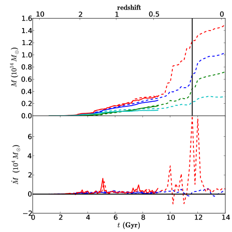
Figure 17: Mass assembly history of galaxy 1, same legend as figure 14. Solid line: level 3 zoom; dashed line: level 2 zoom.

Interestingly, Oser et al. (2010) studied stellar assembly, distinguishing between “in situ” stars that were formed within the galaxy, and “ex situ” stars that were formed in another galaxy before entering the current one. Although these definitions differ somewhat from ours, they are closely related, since “in situ stars” are locally formed from cold gas, and “ex situ” are assembled by mergers. They found that “in situ” stars dominate low mass galaxies at earlier times, while massive galaxies are dominated by “ex situ” star accretion, and in their case the formation of “in situ” stars occurs as the result of the accretion of cold flows. We agree–at least qualitatively–with their evidence of downsizing and observe a similar trend in mean stellar age as a function of galaxy mass, although they have a smaller scatter in the mean stellar age.

Cattaneo et al. (2011) performed a similar analysis using semi-analytical methods. They found that galaxies less massive than $10^{11}\,\mathrm{M}_{\odot}$ assembled most of their mass by mergers rather than by accretion. We qualitatively agree with their results, even though our statistics for massive galaxies are of insufficiently high quality to draw firm conclusions.

Using high-resolution dark matter simulations (the Aquarius project), Wang et al. (2011) also found that mergers with mass ratios larger than 1:10 contribute very little to the DM mass assembly, less than 20%. Most of the major merger contribution is confined to the central parts of haloes, which does not represent the bulk of the mass. This investigation can be extended to baryons, through semi-analytical prescriptions (e.g. Cole et al. 2000; Bower et al. 2006), since the lowest mass halos have a small baryon fraction.

8 Conclusions

We have studied the accretion histories of 530 galaxies using multi-zoom simulations, starting from a cosmological simulation and resimulating three times smaller zones of interest at higher resolution. We selected a dense region and detected the hierarchy of dark matter haloes and subhaloes, as well as baryonic galaxies and satellites, at each timestep of the simulations, which enabled us to follow the structures in time, and build merger trees.

We computed the mass assembled through both smooth gas accretion and mergers, and we found that accretion plays a dominant role, at least until $z\simeq 0.4$, the end of our highest zoom level simulation. Massive galaxies have a lower mass-accretion fraction. Over all galaxies, about three-quarters of the mass is on average assembled through smooth accretion, and one-quarter through mergers. This is in agreement with previous studies examining the role of gas accretion (eg, Murali et al. 2002; Birnboim & Dekel 2003; Semelin & Combes 2005; Kereš et al. 2005, 2009; Brooks et al. 2009; Faucher-Giguère et al. 2011; van de Voort et al. 2011), but we have extended these previous analyses to achieve higher quality statistics.

The main originality of this work lies in the use of multi-zoom simulations, which allow to simulate galaxies with a fairly high resolution in a cosmological context, and to study their mass assembly history. It is worth noting that, even in quite dense environments, where mergers are expected to occur, mass assembly is still dominated by smooth accretion.

We have also studied the evolution of the mass functions of galaxies and DM haloes, especially in dense environments. The galaxy density in our final zoom level is in-between group and cluster environment, and the most massive galaxies are spiral (and not elliptical) at the end of the simulation ($z=0$ at the level 2). This evolution, especially for galaxies, clearly agrees with the hierarchical model, with low-mass galaxies at high redshift and massive ones at low redshift.

We have been able to match DM haloes and galaxies, finding no galaxies without haloe. In contrast, we did find some dark structures containing no galaxies, although this is likely to be an artefact caused by a lack of numerical resolution, and with a higher resolution these galaxies would be detected. We have studied the baryonic content of haloes and found that lower mass haloes have smaller baryon fractions, as expected from the action of stellar feedback. We have studied the evolution of the baryon phases in our simulations, into different components, namely diffuse gas, condensed gas, hot/warm-hot gas, and stars, and distinguishing between the effects of environment and resolution.

Finally, we have studied the mean stellar age of our galaxies, at both $z=0.47$ and $z=0$, and found evidence of downsizing: low mass galaxies form stars at each epoch, whereas in massive galaxies, most stars have formed when the universe was half its present age.

These results however suffer from the problem of overcooling that is encountered at high masses. The downsizing trend should remain detectable despite this problem although the accretion fraction and the gas content of haloes depend on the adopted feedback recipes. The results for the more massive galaxies should thus be taken with caution.

We propose to develop further simulations to explore different physical parameters such as feedback or star formation recipes in order to help us understand their influence on gas accretion as advocated by van de Voort et al. (2011) and Faucher-Giguère et al. (2011). In this next series of simulations, we will be able to address the role of feedback at various epochs in determining the accretion fraction by comparing these simulations with SNe feedback only with our present results.

We note that our present study has been performed on a dense region, and new multi-zoom simulations centred on less dense regions will be analysed to help us ascertain the role of the environment. The relative importance of mergers and diffuse accretion might indeed depend on environment, as Maulbetsch et al. (2007) have shown with dark-matter only simulations. The time scale for the assembly of massive haloes is shorter in dense environments, and the relative role of mergers appears to be higher. Environments with a wide range of densities must therefore be explored by he use of full simulations with baryons and feedback to perform a census of mass assembly encompassing wide ranges of environments and redshifts. The geometry of gas accretion from filaments onto discs will also be studied in more detail.