One-loop corrections, uncertainties and approximations in neutralino annihilations: Examples

F. Boudjema¹⁾, G. Drieu La Rochelle^1),2) and S. Kulkarni³⁾

1) LAPTh^†, Univ. de Savoie, CNRS, B.P.110, Annecy-le-Vieux F-74941, France

2) CERN Physics Department, Theory Division, CH-1211 Geneva 23, Switzerland
3) Bethe Center for Theoretical Physics and Physikalisches Institut, Universität Bonn, Nussallee 12, D-53115 Bonn, Germany

Abstract

The extracted value of the relic density has reached the few per-cent level precision. One can therefore no longer content oneself with calculations of this observable where the annihilation processes are computed at tree-level, especially in supersymmetry where radiative corrections are usually large. Implementing full one-loop corrections to all annihilation processes that would be needed in a scan over parameters is a daunting task. On the other hand one may ask whether the bulk of the corrections are taken into account through effective couplings of the neutralino that improve the tree-level calculation and would be easy to implement. We address this issue by concentrating in this first study on the neutralino coupling to i) fermions and sfermions and ii) $Z$. After constructing the effective couplings we compare their efficiency compared to the full one-loop calculation and comment on the failures and success of the approach. As a bonus we point out that large non decoupling effects of heavy sfermions could in principle be measured in the annihilation process, a point of interest in view of the latest limit on the squark masses from the LHC. We also comment on the scheme dependencies of the one-loop corrected results.

LAPTh-031/11

^†UMR 5108 du CNRS, associée à l’Université de Savoie.

1 Introduction

With barely $1\rm{fb}^{-1}$ of data, the LHC is pushing many hitherto popular, though naive, extensions of supersymmetry to the corners of high masses[1] while leaving some hope for a discovery of a rather light Higgs that could still be compatible with supersymmetry[2]. Before this very recent paradigm, suspersymmetric models (and most models of new physics for that matter) were very strenuously constrained to a thin sliver in parameter space, most notably from the very precise measurement of the dark matter relic density that has now reached the few percent level and that will get even more precise in the future, hence cornering even further model building. Combining the results of the 7-year WMAP data [3] on the 6-parameter $\Lambda$CDM model, the baryon acoustic oscillations from SDSS[4] and the most recent determination of the Hubble constant[5] one[6] arrives at $\Omega_{{\rm CDM}}h^{2}=0.1123\pm 0.0035$, where $\Omega_{{\rm CDM}}$ is the density of cold dark matter normalised to the critical density, and $h$ is the Hubble constant in units of $100$ km s^-1Mpc^-1. One has reached a precision of 3%. The data from the LHC does not infer that dark matter within supersymmetry, exemplified most nicely through the neutralino, the lightest supersymmetric particle (LSP), is of order of 1TeV or so, this is just a limit on the coloured constituents of the model. As for the Higgs, were it not for the large radiative corrections on the mass of the lightest member, supersymmetry would long be a forlorn construct. The Higgs is the most prominent example where radiative corrections are far from negligible in supersymmetry, yet practically all analyses that aim at constraining the parameter space of the MSSM through the relic density are based on tree-level cross sections of the annihilation processes entering the predictions of this quantity which as stressed is experimentally given within the percent accuracy. Only seldom do some analyses assign a theory uncertainty to these annihilation cross sections, an uncertainty due essentially to the fact that higher order loop effects are not known. This uncertainty, in the rare case where it is taken into account, is however assumed to be invariably the same whatever the nature of the dominant process and the composition of the LSP. The reason the loop corrections are ignored, irrespective of the model specified, is that the calculation of the relic density requires most often the evaluation of a large number of processes. Most analyses are done with public codes[7, 8, 9] based on tree-level calculations. Computations of the relic density at one-loop have now been achieved for quite a few channels[10, 11, 12, 13, 14] and tools exist now to perform in principle any calculation of the relic density beyond tree-level amplitudes thanks to the recent development of adapted automation tools[15]. Beside the findings[10, 11, 12, 13, 14] that these corrections are important, the improvements have not percolated to most analyses. It must be said that these calculations do involve some non trivial issues about the renormalisation of the MSSM and more generally techniques for one-loop integrals that certainly require expertise. The other reason is that even when they could be implemented, they are still certainly extremely CPU time consuming, forbidding hence any attempts of fits, likelihood search, and in a more general context any sampling of the parameter space, especially if one takes into account the fact that the MSSM is more than liberal with unconstrained parameters. Yet, apart from providing a more precise prediction, one-loop calculations can probe higher masses, a situation akin to the precision electroweak observables and their sensitivity to the top and Higgs mass. For example, non decoupling effects termed in analogy with electroweak SM observables, super-oblique corrections have been revealed in one-loop calculations of supersymmetry observables[16, 17, 18]. An example in view of the recent findings of the LHC is that super heavy squarks leave a non negligible imprint on many observables in particular the annihilation cross sections involving dark matter.
The aim of this paper is two-fold. First, to stress again the importance of the loop corrections for the relic density and show again that even when a loop calculation is available, there still remains in some cases an uncertainty that pertains to the choice of the renormalisation scheme. The second and more detailed aspect is to discuss whether an approximation to the one-loop calculation can be found. We aim at implementing a universal correction through effective couplings of the LSP and check its validity against a complete one-loop calculation. If such an approximation is possible and general enough it could be implemented in existing codes (based on tree-level cross sections) calculating the relic density. Such was the case with the inclusion of the Sommerfeld effect[19] in the case of coannihilation or processes dominated by Higgs exchange for which $\Delta m_{b}$[20] corrections are included[7].

This preliminary study takes a simple process, namely ${\tilde{\chi}}_{1}^{0}{\tilde{\chi}}_{1}^{0}\rightarrow\mu^{+}\mu^{-}$, as a testing ground. The aim of this study is not to find a good scenario that returns the correct actual value of the relic density but to try to unravel some general common features of the loop calculation to improve the predictions of the relic density. The aim is to rather find out whether one can improve on the tree-level calculation by introducing effective couplings of the LSP that could be used for any process. As we will see, though at first sight naive, the process ${\tilde{\chi}}_{1}^{0}{\tilde{\chi}}_{1}^{0}\rightarrow\mu^{+}\mu^{-}$ embodies the three types of couplings of the neutralino: to $f/\tilde{f}$, gauge bosons and Higgses. Here we cover the bino and the higgsino case. One might argue that the bino case corresponds to what was referred to as the bulk region in the constrained MSSM and is largely ruled out, whereas for a higgsino this would not be the dominant process. As we have just stressed the aim is not to strive to find a good scenario. Besides, it suffices to change the cosmological ingredients[21] entering the calculation of the relic density to revive the so called bulk region. We will see that by considering these few simple examples the conclusions about the efficacy of the effective coupling is quite different. Moreover, there is no need here to convert a full corrected cross section into a relic density value, we rather take for all the models we study the annihilation cross section for an energy corresponding to a relative velocity of $v=0.2$, typical for the relic density calculation. As known, for zero relative velocity the process enjoys chirality suppression which is lifted at higher order through gauge boson radiation, however the effect on the relic is totally marginal[10].

The paper is organised as follows. We first briefly describe the ingredients necessary to perform a one-loop calculation in supersymmetry covering both automation, renormalisation and renormalisation schemes, it is in this section that we will write down the effective universal neutralino couplings as well as some definitions. Section 3 contains our main results. After a few definitions we first study the case of a bino-like neutralino before addressing the case of a higgsino-like LSP. We also quantify the possible uncertainties due to the scheme dependence. We conclude in Section 4 by some general observations.
Throughout the paper we use some shorthand notation for angles. Generically $c_{\theta},s_{\theta},t_{\theta}$ stand for $\cos\theta,\sin\theta,\tan\theta$. The weak mixing angle $\theta_{W}$ is defined as $\cos\theta_{W}=c_{W}=M_{W}/M_{Z}$ where $M_{W}$ is the $W$ mass and $M_{Z}$ the $Z$ mass.

2 Calculations, renormalisation, schemes at full one-loop

2.1 Tree-level considerations

$(a)$	$(b)$	$(c)$

Figure 1: Tree-level diagrams contributing to ${\tilde{\chi}}_{1}^{0}{\tilde{\chi}}_{1}^{0}\rightarrow\mu^{+}\mu^{-}$. ($a$) is the $t$-channel $\tilde{\mu}$ exchange, ($b$) is the $Z$ exchange and ($c$) an example of a Higgs exchange.

At tree-level, see Fig. 1, ${\tilde{\chi}}_{1}^{0}{\tilde{\chi}}_{1}^{0}\to\mu^{+}\mu^{-}$ proceeds through i) $t$-channel smuon exchange dominated by a $\tilde{\mu}_{R}$ in the case of a bino-like since it has the largest hypercharge, ii) a $Z$ exchange which, on the other hand, is suppressed for the bino iii) Higgs exchange but this is small in view of the Yukawa coupling of the muon. Therefore, as advertised, all types of couplings for the LSP are present: to fermions in the ${\tilde{\chi}}_{1}^{0}\tilde{\mu}\mu$ coupling, gauge bosons in the ${\tilde{\chi}}_{1}^{0}{\tilde{\chi}}_{1}^{0}Z$, and Higgs scalars such as ${\tilde{\chi}}_{1}^{0}{\tilde{\chi}}_{1}^{0}A^{0}$ ($A^{0}$ is the pseudoscalar Higgs). It is through the choice of a hierarchy in the set $M_{1},M_{2},\mu$ that we can largely define the nature of the LSP. Numericaly speaking we call a neutralino pure or almost pure when its mixing to the specified species is over 99%.

2.2 Renormalisation and loop corrections, general considerations and issues

2.2.1 Set up of the automatic calculation: SloopS

One-loop processes calculated via the diagrammatic Feynman approach involve a huge number of diagrams even for $2\rightarrow 2$ reactions, especially in a theory like supersymmetry. Performing a full one-loop calculation by hand without automation is practically untractable. Our exact full one-loop calculation is done with the help of the automated code SloopS. SloopS is an automated code for one-loop calculations in supersymmetry. It is a combination of LanHEP[22], the bundle FeynArts[23], FormCalc[24] and an adapted version of LoopTools[25, 26]. LanHEP deals with one of the main difficulties that has to be tackled for the automation of the implementation of the model file, which is entering the thousands of vertices that define the Feynman rules. On the theory side a proper renormalisation scheme needs to be set up, which then means extending many of these rules to include counter-terms. This part is done through LanHEP which allows to shift fields and parameters and thus generates counterterms most efficiently. The ghost Lagrangian is derived directly from the BRST transformations. The loop libraries used in SloopS are based on LoopTools with the addition of quite a few routines in particular those for dealing with small Gram determinants that appear in our case at small relative velocities of the annihilating dark matter, and even more so of relevance for indirect detection[26].

2.2.2 Renormalisation

In SloopS all sectors of the MSSM are implemented through a one-loop renormalisation. This is explained in details in[10, 27, 28, 13]. Here we only briefly sketch the renormalisation procedure. We have worked, as far as possible, within an on-shell scheme generalising what is done for the electroweak standard model[29].

i) The Standard Model parameters : the fermion masses as well as the mass of the W and Z are taken as input physical parameters. The electric charge is defined in the Thomson limit, see for example[29]. The light quarks (effective) masses are chosen [30] such as to reproduce the SM value of $\alpha^{-1}(M_{Z}^{2})$ = 127.77. This should be kept in mind since one would be tempted to use a ${\overline{\rm DR}}$ scheme for $\alpha$, defined as $M_{Z}$, to take into account the fact that dark matter is annihilating at roughly the electroweak scale, so that $\alpha((2m_{{\tilde{\chi}}_{1}^{0}})^{2})$ is a more appropriate choice. One should remember that the use of $\alpha((2m_{{\tilde{\chi}}_{1}^{0}})^{2})$ instead of the on-shell value in the Thomson limit would correct the tree-level cross section for ${\tilde{\chi}}_{1}^{0}{\tilde{\chi}}_{1}^{0}\rightarrow\mu^{+}\mu^{-}$ by about $14\%$. As we will see and have reported somewhere else for other processes this running does not, most of the time, take into account the bulk of the radiative corrections that we report here. Therefore for further reference, let us introduce the correction due to the running of $\alpha$,

$$\Delta_{\alpha}=\frac{\sigma_{\alpha\textrm{eff}}-\sigma_{0}}{\sigma_{0}}=2\Delta\alpha,$$ (1)

where the cross section $\sigma_{0}$ is the tree-level calculated with $\alpha_{0}=\alpha(0)=1/137.0359895$ whereas $\sigma_{\alpha\textrm{eff}}$ is the tree-level with $\alpha_{0}\rightarrow\alpha_{\rm eff.}(Q^{2})=\alpha(Q^{2})=\alpha_{0}/(1+\Delta\alpha(Q^{2})),Q=2m_{{\tilde{\chi}}_{1}^{0}}$. With our input parameters $\Delta\alpha(M_{Z}^{2})=0.06$. In the running we allow for all charged particles including the $W$ boson contribution, the top and the sfermions and the charginos, though for the light LSP scenario we consider these added contributions are very small

ii) The Higgs sector : The pseudoscalar Higgs mass $M_{A}^{0}$ is used as an input parameter while insisting on vanishing tadpoles. $t_{\beta}$, which at tree-level is the ratio of the two expectation values of the Higgs doublets, can be defined through several schemes:

 -

In the DCPR scheme[31, 32] $t_{\beta}$ is defined by requiring that the (renormalised) $A^{0}Z$ transition vanishes at $Q^{2}=M_{A^{0}}^{2}$.

 -

a ${\overline{\rm DR}}$ definition where the $t_{\beta}$ counter-term, $\delta t_{\beta}$, is defined as a pure divergence leaving out all finite parts.

 -

a process-dependent definition of this counter-term by extracting it from the decay $A^{0}\rightarrow\tau^{+}\tau^{-}$ that we will refer to as ${\mathrm{A}_{\tau\tau}}$ for short. This definition is a good choice for the gauge independence of the processes.

 -

an on-shell definition with the help of the mass of the heavy CP Higgs $H$ taken as input parameter called the MH scheme from now on. We have reported elsewhere that this scheme usually introduces large radiative corrections.

These schemes are critically reviewed in [27]. By default we use the DCPR scheme but when quantifying the effect of the scheme dependence on $t_{\beta}$ we also use the ${\overline{\rm DR}}$ and MH scheme.

iii) The sfermion sector : For the process at hand only the smuons parameters require renormalisation. For the slepton sector we use as input parameters masses of the two charged sleptons which in the case of no-mixing define the R-slepton soft breaking mass, $M_{{\tilde{\mu}}_{R}}$ and the $SU(2)$ mass, $M_{{\tilde{\mu}}_{L}}$, giving a correction to the sneutrino mass at one-loop. Though not needed here, in the squark sector each generation needs three physical masses to constrain the breaking parameter $M_{{\tilde{Q}}_{L}}$ for the $SU(2)$ part, $M_{{\tilde{u}}_{R}}$, $M_{{\tilde{d}}_{R}}$ for the R-part. See[28] for details.

iv) The chargino/neutralino sector. First of all, for the neutralinos at tree-level the physical fields $\chi^{0}_{i},i=1,\dots,4$ are obtained from the current eigenstates $\big{(}\psi^{n}\big{)}^{t}=(\tilde{B}^{0},\tilde{W}^{0},\tilde{H}_{1}^{0},\tilde{H}_{2}^{0})$ through a unitary complex matrix $N$

$$\chi^{0}=N\psi^{n}.$$ (2)

$N$ diagonalises the mass mixing matrix $Y$ in the neutralino sector, see [28] for details and conventions. Although only ${\tilde{\chi}}_{1}^{0}$ enters our calculations we do need to fix all the elements that define its composition and hence couplings. For this sector we implement an on-shell scheme by taking as input three masses in order to reconstruct the underlying parameters $M_{1},M_{2},\mu$. In SloopS [28] the default scheme is to choose two charginos masses $m_{{\tilde{\chi}}_{1}^{\pm}}$ and $m_{{\tilde{\chi}}_{2}^{\pm}}$ as input to define $M_{2}$ and $\mu$ and one neutralino mass to fix $M_{1}$. The masses of the remaining three neutralinos receive one-loop quantum corrections. In this scheme, these counterterms are [28]

$$\delta M_{2} = \frac{1}{M_{2}^{2}-\mu^{2}}\left((M_{2}m_{\tilde{\chi}_{1}^{+}}^{2}-\mu{\rm det}X)\frac{\delta m_{\tilde{\chi}_{1}^{+}}}{m_{\tilde{\chi}_{1}^{+}}}+(M_{2}m_{\tilde{\chi}_{2}^{+}}^{2}-\mu{\rm det}X)\frac{\delta m_{\tilde{\chi}_{2}^{+}}}{m_{\tilde{\chi}_{2}^{+}}}\right.$$

$$-\left.M_{W}^{2}(M_{2}+\mu s_{2\beta})\frac{\delta M_{W}^{2}}{M_{W}^{2}}-\mu M_{W}^{2}s_{2\beta}c_{2\beta}\frac{\delta t_{\beta}}{t_{\beta}}\right),$$

$$\delta\mu = \frac{1}{\mu^{2}-M_{2}^{2}}\left((\mu m_{\tilde{\chi}_{1}^{+}}^{2}-M_{2}{\rm det}X)\frac{\delta m_{\tilde{\chi}_{1}^{+}}}{m_{\tilde{\chi}_{1}^{+}}}+(\mu m_{\tilde{\chi}_{2}^{+}}^{2}-M_{2}{\rm det}X)\frac{\delta m_{\tilde{\chi}_{2}^{+}}}{m_{\tilde{\chi}_{2}^{+}}}\right.$$ (3)

$$-\left.M_{W}^{2}(\mu+M_{2}s_{2\beta})\frac{\delta M_{W}^{2}}{M_{W}^{2}}-M_{2}M_{W}^{2}s_{2\beta}c_{2\beta}\frac{\delta t_{\beta}}{t_{\beta}}\right),$$

$$\delta M_{1} = \frac{1}{N_{1i}^{2}}(\delta m_{\chi_{i}^{0}}-N_{2i}^{2}\delta M_{2}+2N_{3i}N_{4i}\delta\mu$$ (4)

$$-2N_{1i}N_{3i}\delta Y_{13}-2N_{2i}N_{3i}\delta Y_{23}-2N_{1i}N_{4i}\delta Y_{14}-2N_{2i}N_{4i}\delta Y_{24})\,,$$

with $\textrm{det}X=M_{2}\mu-M_{W}^{2}s_{2\beta}$ [28]. $\delta m_{\tilde{\chi}_{i}^{0}}$ is the counterterm of $i$th neutralino defined entirely from its self-energy, see[28]. $\delta O$ represents the shift on the parameter $O$ that generates the counterterm for that quantity.
Looking at these equations some remarks can be made. First, in the special configuration $M_{2}\sim\pm\mu$ an apparent singularity might arise. Ref. [10] pinpointed this configuration which can induce a large $t_{\beta}$-scheme dependence in the counterterms $\delta M_{1,2}$ and $\delta\mu$. Such mixed scenario is not covered here.
Second, the choice of $m_{{\tilde{\chi}}_{1}^{0}}$ as an input parameter is appropriate only if the lightest neutralino is mostly bino ($|N_{11}|\sim 1$) or if the bino like neutralino is not too heavy compared to other neutralinos. Indeed we can see that if $N_{1i}\sim 0$ the counterterm $\delta M_{1}$ is subject to large uncertainty and may introduce large finite correction, this is related to the fact that $M_{1}$ is badly reconstructed. To avoid such uncertainty we only choose $i$ as the most bino like, in other words in Eq. 4, $|N_{1i}|=Max(|N_{1j}|),j=1,..4$.

v) Finally diagonal field renormalisation is fixed by demanding that the residue at the pole of the propagator of all physical particles to be unity, and the non-diagonal part by demanding no-mixing between the different physical particles when on shell. This is implemented in all the sectors. In our case apart from the muon, this step is important for the ${\tilde{\chi}}_{1}^{0}$. We insist that $N_{ij}$ is used both at the tree-level and one-loop level. Nonetheless to define the physical state we do introduce the shift for the neutralinos[28] through wave function renormalisation

$$\tilde{\chi}_{i}^{0}\to\tilde{\chi}_{i}^{0}+\frac{1}{2}\sum_{j}\left(\delta Z_{ij}P_{L}+\delta Z^{*}_{ij}P_{R}\right)\tilde{\chi}_{j}^{0}\,.$$ (5)

vi) Dimensional reduction is used as implemented in the FFL bundle at one-loop through the equivalent constrained dimensional renormalisation[33].

2.2.3 Infrared divergences

For the processes ${\tilde{\chi}}_{1}^{0}{\tilde{\chi}}_{1}^{0}\rightarrow\mu^{+}\mu^{-}$, we can decompose the one-loop amplitudes in a virtual part $\mathcal{M}_{1loop}^{EW}$ and a counter-term contribution $\mathcal{M}_{CT}$. The sum of these two amplitudes must be ultraviolet finite and gauge independent. Due to the virtual exchange of the massless photon, this sum can contain infrared divergencies. This is cured by adding a small mass to the photon and/or gluon, $\lambda_{\gamma}$ and $\lambda_{g}$. This mass regulator should exactly cancel against the one present in the final state radiation of a photon. The QED contribution is therefore split into two parts : a soft one where the photon energy $E_{\gamma}$ is integrated to less than some small cut-off $k_{c}$ and a hard part with $E_{\gamma}>k_{c}$. The former requires a photon mass regulator. Finally the sum $\mathcal{M}_{1loop}+\mathcal{M}_{CT}+\mathcal{M}_{\gamma}^{soft}(E_{\gamma}<k_{c})+\mathcal{M}_{\gamma,g}^{hard}(E_{\gamma,g}>k_{c})$ should be ultraviolet finite, gauge invariant, not depend on the mass regulator and on the cut $k_{c}$.

2.2.4 Checking the result

i) For each process and set of parameters, we first check the ultraviolet finiteness of the results. This test applies to the whole set of virtual one-loop diagrams. The ultraviolet finiteness test is performed by varying the ultraviolet parameter $C_{UV}=1/\varepsilon$, $\varepsilon$ is the usual regulator in dimensional reduction. We vary $C_{UV}$ by seven orders of magnitude with no change in the result. We content ourselves with double precision.

ii) The test on the infrared finiteness is performed by including both the loop and the soft bremsstrahlung contributions and checking that there is no dependence on the fictitious photon mass $\lambda_{\gamma}$.

iii) Gauge parameter independence of the results is essential. It is performed through a set of the eight gauge fixing parameters based on the implementation of a non-linear gauge[27].

2.3 Effective couplings for neutralino interactions vs Full calculation

2.3.1 Contributions at full one-loop

(a)	(b)	(c)

Figure 2: Different types of corrections appearing at one-loop for the process ${\tilde{\chi}}_{1}^{0}{\tilde{\chi}}_{1}^{0}\rightarrow\mu^{+}\mu^{-}$. ($a$) is the correction to vertex ${\tilde{\chi}}_{1}^{0}\mu\tilde{\mu}$ for the $t$-channel $\tilde{\mu}$ exchange, ($b$) is the full correction to the ${\tilde{\chi}}_{1}^{0}{\tilde{\chi}}_{1}^{0}Z$ vertex for the $s$-channel $Z$ exchange and ($c$) is an example of a box loop.

The full set of one-loop contributions to the process ${\tilde{\chi}}_{1}^{0}{\tilde{\chi}}_{1}^{0}\rightarrow\mu^{+}\mu^{-}$ consist of two-point functions (self-energies and transitions such as ${\tilde{\chi}}_{1}^{0}\rightarrow{\tilde{\chi}}_{2}^{0}$), vertex three-point functions as in Figs 2(a,b) and box diagrams. The vertex corrections include also the counterterms, the latter as explained previously involve two-point functions. To these, one should also add the QED final state radiation.

2.3.2 Effective couplings of the neutralino at one-loop

Among this full set of corrections one can construct a finite subset that is not specific to the muon. This subset will be involved in all processes involving neutralinos. For example, the vertex correction to ${\tilde{\chi}}_{1}^{0}{\tilde{\chi}}_{1}^{0}Z$ is obviously independent of the muon being in the final state, a similar statement can be said for ${\tilde{\chi}}_{1}^{0}{\tilde{\chi}}_{1}^{0}h/H/A$. Also, all occurrences of the wave function renormalisation of the neutralino (including transitions between neutralinos) and the $Z$ are process independent. The same can be said also of the counterterms to the gauge couplings and the vacuum expectation values or in other words $v,t_{\beta}$. On the other hand the wave function renormalisation of the muon is specific to the muon final state. The boxes the four-point one particle irreducible (1-PI) functions, as well as the QED correction are also specific to the process. The construct of the universal correction for the effective coupling ${\tilde{\chi}}_{1}^{0}f\tilde{f}$ from ${\tilde{\chi}}_{1}^{0}\mu\tilde{\mu}$ is different from that of ${\tilde{\chi}}_{1}^{0}{\tilde{\chi}}_{1}^{0}Z$, since in the latter all three particles can be considered as universal. For example the full correction to the vertex ${\tilde{\chi}}_{1}^{0}\mu\tilde{\mu}$ shown in Fig. 2(a), consists of a 1-PI 3-point function vertex correction (triangle) which is muon specific and that does not need to be calculated to build up the effective coupling. It also contains wave function renormalisation of the neutralinos as well as counterterms for the gauge couplings and for other universal quantities such as $t_{\beta}$ which must be combined to arrive at the universal correction for the ${\tilde{\chi}}_{1}^{0}f\tilde{f}$ vertex. The aim of the paper is therefore to extract these process independent contributions and define effective vertices for the LSP interactions. This is akin to the effective coupling of the $Z$ to fermions where universal corrections are defined. Describing the bulk of the radiative corrections in terms of effective couplings has been quite successful to describe for example the observables at the $Z$ peak. Although not describing most perfectly the effect of the full corrections for all observables (for example $Zb\bar{b}$ receives an important triangle contribution due to the large top Yukawa coupling) one must admit that the approach has done quite a good job. Most of the effective corrections were universal, described in terms of a small set of two-point functions of the gauge bosons.
The other benefit was that such approximations were sensitive to non decoupling effects that probe higher scales (top mass and Higgs mass). The set of two-point functions, and for ${\tilde{\chi}}_{1}^{0}{\tilde{\chi}}_{1}^{0}Z$ three-point functions, should of course lead to a finite and gauge invariant quantity. Loops involving gauge bosons have always been problematic (even in the case of the $Zf\bar{f}$) in such an approach since it is difficult to extract a gauge independent value. For the couplings of the neutralinos as would be needed for approximating their annihilation cross section independently of the final state, one would therefore expect that apart from the rescaling of the gauge couplings which can be considered as an overall constant, the mixing effect between the different neutralinos should be affected. One can in fact re-organise a few of the two point functions (that can be written also as counterterms) to define an effective coupling for the neutralino. One should of course also correct in this manner the $Z\mu^{+}\mu^{-}$ coupling. Let us stress again that in this first investigation we will primarily take into account the effects of fermions and sfermions in the universal loops. For the ${\tilde{\chi}}_{1}^{0}{\tilde{\chi}}_{1}^{0}Z$ effective we also attempt to include the virtual contribution of the gauge bosons especially that for the higgsino-like the coupling to $W$ and $Z$ are not suppressed.

2.3.3 The effective ${\tilde{\chi}}_{1}^{0}f\tilde{f}$

To find the process independent corrections to this coupling, we recall that in the basis $(\tilde{B}^{0},\tilde{W}^{0},\tilde{H}_{1}^{0},\tilde{H}_{2}^{0})$ before mixing and for both $f_{L,R}$ the couplings for the two chiral Lorentz structures writes as

$$\frac{1}{\sqrt{2}}\big{(}g^{\prime}Y_{f},g\tau^{3}_{f},y_{1,f},y_{2,f}\big{)}=\frac{1}{\sqrt{2}}\big{(}g^{\prime}Y_{f},g\tau^{3}_{f},\frac{gm_{u}}{M_{W}c_{\beta}},\frac{gm_{d}}{M_{W}s_{\beta}}\big{)}\rightarrow\big{(}g^{\prime},g,\frac{g}{M_{W}c_{\beta}},\frac{g}{M_{W}s_{\beta}}\big{)},$$ (6)

$Y_{f},\tau_{3}^{f}$ are the isospin and $SU(2)$ charges of the corresponding fermion/sfermions. The two higgsinos couple differently to the up and down fermions with a coupling that is proportional to the Yukawa coupling. Though this is not universal we can still isolate a universal part where there is no reference to the final fermion/sfermion. This is what is meant by the last expression in Eq. 6 where the explicit mass of the corresponding fermion masses has been dropped. The variations/counterterms on these parameters have to be implemented before turning to the physical basis. The latter as explained in the previous paragraph is achieved through the diagonalising matrix $N$ (Eq. 2) as in tree-level supplemented by wave function renormalisation which involve both diagonal and non diagonal transitions of the neutralino, see Eq. 5. In the case of effective coupling of neutralinos, this is achieved by defining an effective mixing matrix such that $N\rightarrow N+\Delta N^{\chi f\tilde{f}}$ in all couplings of the neutralino. The $\Delta N^{\chi f\tilde{f}}$ write as

$$\Delta N_{i1}^{\chi f\tilde{f}} = \frac{\delta g^{\prime}}{g^{\prime}}N_{i1}+\frac{1}{2}\sum_{j}N_{j1}\delta Z_{ji},$$

$$\Delta N_{i2}^{\chi f\tilde{f}} = \frac{\delta g}{g}N_{i2}+\frac{1}{2}\sum_{j}N_{j2}\delta Z_{ji},$$

$$\Delta N_{i3}^{\chi f\tilde{f}} = \left(\frac{\delta g}{g}-\frac{1}{2}\frac{\delta M_{W}^{2}}{M_{W}^{2}}-\frac{\delta c_{\beta}}{c_{\beta}}\right)N_{i3}+\frac{1}{2}\sum_{j}N_{j3}\delta Z_{ji},$$

$$\Delta N_{i4}^{\chi f\tilde{f}} = \left(\frac{\delta g}{g}-\frac{1}{2}\frac{\delta M_{W}^{2}}{M_{W}^{2}}-\frac{\delta s_{\beta}}{s_{\beta}}\right)N_{i4}+\frac{1}{2}\sum_{j}N_{j4}\delta Z_{ji}.$$ (7)

where $j$ runs from 1 to 4 and for the LSP , $i=1$.

All the counterterms above are calculated from self-energy two-point functions and are fully defined in  [27, 28]. $\delta g/g=\delta e/e-\delta s_{W}/s_{W},\delta g^{\prime}/g^{\prime}=\delta e/e-\delta c_{W}/c_{W}$. $\delta s_{\beta}/s_{\beta}=c_{\beta}^{2}\delta t_{\beta}/t_{\beta}$. Eq. 2.3.3 agrees with what was suggested in [34]. Let us stress again that in these self-energies no gauge bosons and therefore no neutralinos and charginos are taken into account but just sfermions and fermions, otherwise this would not be finite. For a bino-like, self-energies containing gauge and Higgs bosons (with their supersymmetric conterparts) are not expected to contribute much. This is not necessarily the case for winos and higgsinos.

2.3.4 The effective ${\tilde{\chi}}_{1}^{0}{\tilde{\chi}}_{1}^{0}Z$

Since all particles making this vertex can now be considered as being process independent (as far as neutralino annihilations are concerned), all counterterms including wave function renormalisation of both the $Z$ and ${\tilde{\chi}}_{1}^{0}$ must be considered. The price to pay now is that the genuine triangle vertex corrections ${\tilde{\chi}}_{1}^{0}{\tilde{\chi}}_{1}^{0}Z$ must also be included. It is only the sum of the vertex and the self-energies that renders a finite result. When correcting this vertex one must also correct the $Z\mu^{+}\mu^{-}$ vertex keeping within the spirit of calculating the universal corrections. This can be implemented solely through self-energy corrections (excluding the muon self-energies) and there is no need to calculate here the genuine vertex corrections. An exception would be the production of the $b$ and to some extent the top where genuine vertex corrections are important. Talking of heavy flavours, when computing the correction to the ${\tilde{\chi}}_{1}^{0}{\tilde{\chi}}_{1}^{0}Z$ with the Z off shell with an invariant mass $Q^{2}$, one should also include the ${\tilde{\chi}}_{1}^{0}{\tilde{\chi}}_{1}^{0}G^{0}$ vertex, where $G^{0}$ is the neutral Goldstone boson. In our case we restrict ourselves to almost massless fermions. The case of the top and bottom final states will be addressed elsewhere together with the potential relevant contribution of the Higgses in the $s$-channel.
Since one is including the genuine 1-PI vertex correction, it is important to inquire whether this correction generates a new Lorentz structure beyond the one found at tree-level. The contribution to the tree-level Lorentz structure is finite after adding the self-energies and the vertex. Any new Lorentz structure will on the other hand be finite on its own. General arguments based on the Majorana nature of the neutralinos backed by our numerical studies show that no new Lorentz structure is generated for neutralinos. First of all, at tree-level one has only one structure

$${\cal{L}}_{{\tilde{\chi}}_{1}^{0}{\tilde{\chi}}_{1}^{0}Z}=\frac{g_{Z}}{4}\Big{(}N_{13}N_{13}-N_{14}N_{14}\Big{)}{\tilde{\chi}}_{1}^{0}\gamma_{\mu}\gamma_{5}{\tilde{\chi}}_{1}^{0}Z^{\mu},\quad\quad g_{Z}=\frac{e}{c_{W}s_{W}}.$$ (8)

The overall strength is a consequence of the fact that the coupling emerges solely from the higgsino with a gauge coupling. Indeed in the $(\tilde{B}^{0},\tilde{W}^{0},\tilde{H}_{1}^{0},\tilde{H}_{2}^{0})$ basis the coupling is $\propto g_{Z}(0,0,1,-1)$. Only the Lorentz structure $\gamma_{\mu}\gamma_{5}$ survives as a consequence of the Majorana nature. With $p_{1},p_{2}$ denoting the incoming momenta of the two ${\tilde{\chi}}_{1}^{0}$, at one-loop a contribution $(p_{1}^{\mu}-p_{2}^{\mu})$ does not survive symmetrisation, whereas $(p_{1}^{\mu}+p_{2}^{\mu})$ will not contribute for massless muons. We calculate this correction for a $Z$ with an invariant mass $Q^{2}$, in the application this $Q^{2}$ will be set to the invariant mass of the muon pair. This vertex contribution is denoted $\Delta g_{{\tilde{\chi}}_{1}^{0}{\tilde{\chi}}_{1}^{0}Z}^{\bigtriangleup}(Q^{2})\equiv\Delta g_{{\tilde{\chi}}_{1}^{0}{\tilde{\chi}}_{1}^{0}Z}^{\bigtriangleup}$. The contribution of the coupling counterterms defining $g_{Z}$ and the $Z$ wave function renormalisation define the universal correction to the $Z$ coupling strength $g_{Z}^{\rm eff}=g_{Z}(1+\Delta g_{Z})$, with $\Delta g_{Z}/g_{Z}=\delta g_{Z}/g_{Z}+\delta Z_{ZZ}/2$. $\delta Z_{ZZ}$ is the wave function renormalisation of the $Z$. We of course have to add the wave function renormalisation of the ${\tilde{\chi}}_{1}^{0}$ like what was done for the ${\tilde{\chi}}_{1}^{0}f\tilde{f}$ vertex. We improve on this implementation by taking into account the fact that the $Z$ is off-shell and therefore the wave function renormalisation through $\delta Z_{ZZ}=\Pi_{ZZ}^{\prime}(M_{Z}^{2})$ is only part of the correction that would emerge from the correction to the complete $Z$ propagator in the $s$-channel contribution with invariant mass $Q^{2}$. Note that here there is no need for including a $Z\gamma$ transition since photons do not couple to neutralinos. Collecting all these contributions, the effective vertex is obtained by making
$g_{Z}\to g_{{\tilde{\chi}}_{1}^{0}{\tilde{\chi}}_{1}^{0}Z}^{{\rm eff}}$ and $N_{i1}\to N_{i1}+\Delta N_{i1}^{{\tilde{\chi}}_{1}^{0}{\tilde{\chi}}_{1}^{0}Z}$ with

$$g_{{\tilde{\chi}}_{1}^{0}{\tilde{\chi}}_{1}^{0}Z}^{{\rm eff}} = g_{Z}(1+\Delta g_{Z}(Q^{2})+\Delta g_{{\tilde{\chi}}_{1}^{0}{\tilde{\chi}}_{1}^{0}Z}^{\bigtriangleup}(Q^{2}));$$ (9)

$$\quad\Delta N_{ij}^{{\tilde{\chi}}_{1}^{0}{\tilde{\chi}}_{1}^{0}Z} = \frac{1}{2}\sum_{k}N_{kj}\delta Z_{ki},\;\;(i,j,k)=1\dots 4.$$ (10)

Explicitly

$$\Delta g_{Z} = \frac{1}{2}\left(\Pi^{\prime}_{\gamma\gamma}(0)-2\frac{s_{W}}{c_{W}}\frac{\Pi_{\gamma Z}(0)}{M_{Z}^{2}}\right)+\frac{1}{2}\left(1-\frac{c_{W}^{2}}{s_{W}^{2}}\right)\left(\frac{\Pi_{ZZ}(M_{Z}^{2})}{M_{Z}^{2}}-\frac{\Pi_{WW}(M_{W}^{2})}{M_{W}^{2}}\right)$$ (11)

$$- \frac{1}{2}\left(\frac{\Pi_{ZZ}(Q^{2})-\Pi_{ZZ}(M_{Z}^{2})}{Q^{2}-M_{Z}^{2}}\right)\ .$$

At the same time for the fermion with charge $q_{f}$ we correct the $Zf\bar{f}$ $\propto g_{Z}(\gamma_{5}+(1-4|q_{f}|s_{W}^{2}))\gamma_{\mu}$ by effectively making $g_{Z}\to g_{Z}(1+\Delta g_{Z})$ with $\Delta g_{Z}$ defined in Eq. 11 and $s_{W}^{2}$ to

$$\Delta s_{W}^{2}=\frac{c_{W}^{2}}{s_{W}^{2}}\left(\frac{\Pi_{ZZ}(M_{Z}^{2})}{M_{Z}^{2}}-\frac{\Pi_{WW}(M_{W}^{2})}{M_{W}^{2}}\right)+\frac{c_{W}}{s_{W}}\frac{\Pi_{\gamma Z}(k^{2})}{k^{2}}\ .$$ (12)

By default we include only the fermions and sfermions in the virtual corrections described by Eqs. 11-12. For the ${\tilde{\chi}}_{1}^{0}{\tilde{\chi}}_{1}^{0}Z$ one expect the contribution of the gauge bosons and the neutralinos/charginos to be non negligible especially for the higgsino case. In fact, including such contributions still gives an ultraviolet finite result for $g_{{\tilde{\chi}}_{1}^{0}{\tilde{\chi}}_{1}^{0}Z}^{{\rm eff}}$ in Eq. 11 which is a non trivial result. Moreover this contribution is gauge parameter independent in the class of (linear) and non-linear gauge fixing conditions[29]. To weigh up the gauge/gaugino/higgsino contribution we will therefore also compare with this generalised effective $g_{{\tilde{\chi}}_{1}^{0}{\tilde{\chi}}_{1}^{0}Z}^{{\rm eff}}$ including all virtual particles. Observe that in Eq. 11 we have the contribution $\Pi_{\gamma Z}(0)$ which vanishes for fermions and sfermions but which is essential for the contribution of the virtual $W$. In any case including gauge bosons in the renormalisation of electromagnetic coupling requires the inclusion of the $\Pi_{\gamma Z}(0)$ in Eq. 11 for gauge invariance to be maintained[29]. We stress that we will present the effect of the generalised effective coupling $g_{{\tilde{\chi}}_{1}^{0}{\tilde{\chi}}_{1}^{0}Z}^{{\rm eff}}$ as an indication of the gauge boson contribution while keeping in mind that this result may lead to unitarity violation. Indeed through cutting rules, the $W$ loop can be seen as made up of the scattering $W^{+}W^{-}\to Z\to\mu^{+}\mu^{-}$ that needs a compensation from the cut in the box shown in Fig. 2(c). For the effective $Z\mu^{+}\mu^{-}$ coupling we only include the fermion/sfermion contribution in Eqs. 11-12, adding the gauge bosons would require part of the 1-PI triangle contribution to $Z\to\mu^{+}\mu^{-}$.

3 Analysis

Since we will be studying different compositions of the neutralinos we will take different values for the set $M_{1},M_{2},\mu$. On the other hand the default parameters in the Higgs sector are

$$M_{A^{0}}=1{\rm TeV}\quad\quad t_{\beta}=4.$$ (13)

The sfermion sector is specified by a rather heavy spectrum (in particular within the limits set by the LHC for squarks[1]). All sleptons left and right of all generations have a common mass which we take to be different from the common mass in the squark sector. All tri-linear parameters $A_{f}$ (including those for stops and sbottom) are set to 0. The default values for the sfermion masses are

$$M_{{\tilde{l}}_{R}} = M_{{\tilde{l}}_{L}}=500{\rm GeV},$$

$$M_{{\tilde{u}}_{R}} = M_{{\tilde{d}}_{R}}=M_{{\tilde{Q}}_{L}}=800{\rm GeV},$$

$$A_{f} = 0\,.$$ (14)

By default we will focus on relatively light neutralinos (around 100 GeV) scattering with a relative velocity $v=0.2$.

To analyse consistently the efficiency of effective corrections we will refer to the following quantities :

$$\Delta_{\rm eff}=\frac{\sigma_{\textrm{eff}}-\sigma_{0}}{\sigma_{0}}\,.$$ (15)

Here $\sigma_{\textrm{eff}}$ is the cross section calculated with the effective couplings that include, by default, universal process independent particles excluding gauge bosons and gauginos/higgsinos. We will explicitely specify when including all virtual particles in those corrections, referring to it as $\Delta_{\rm eff}^{W}$. This correction will be compared to the correction solely due to the running of the electromagnetic coupling, see Eq. 1. To see how well the correction through the effective couplings ${\tilde{\chi}}_{1}^{0}f\tilde{f}$ and ${\tilde{\chi}}_{1}^{0}{\tilde{\chi}}_{1}^{0}Z$ reproduces the full one-loop correction we introduce

$$\Delta_{NU}=\frac{\sigma_{\textrm{one-loop}}-\sigma_{\textrm{eff}}}{\sigma_{0}}\,,$$

$$\Delta_{\rm full}=\frac{\sigma_{\textrm{one-loop}}-\sigma_{0}}{\sigma_{0}}\;.$$ (16)

with $\sigma_{\textrm{one-loop}}$ the full one-loop cross section, $\Delta_{NU}$ measures what we will refer to as the non-universal corrections although strictly speaking this measures the remainder of all the corrections that are not taken into account by the effective vertices approach. $\Delta_{\rm full}=\Delta_{\rm eff}+\Delta_{NU}$ is the full one-loop correction.

3.1 Bino Case

3.1.1 Effective vs full corrections

We first take $(M_{1},M_{2},\mu)=(90,200,-600)\ GeV$ which yields a lightest bino-like neutralino (the bino composition is 99%) with mass $m_{{\tilde{\chi}}_{1}^{0}}=91\ GeV$. At tree-level the cross section for relative velocity $v=0.2$ is $\sigma_{\mu^{+}\mu^{-}}^{\tilde{b}}=6.75\times 10^{-3}{\rm pb}$. Note for further reference that this is an order of magnitude larger than annihilation into a pair of $W$’s: $\sigma_{W^{+}W^{-}}^{\tilde{b}}=4.51\times 10^{-4}{\rm pb}$. The annihilation proceeds predominantly through the $t$-channel, binos coupling to $Z$ are very much reduced. This leads to the following set of corrections

$$\Delta_{\rm eff}=17.52\%(\Delta_{\alpha}=14.56\%)\quad\quad\Delta_{NU}=2.06\%(\Delta_{\rm full}=19.58\%).$$ (17)

For our first try the effective universal coupling does remarkably well falling short of only $2\%$ correction compared to the full calculation. Note that although the most naive implementation through a running of the electromagnetic coupling fares also quite well it is nonetheless $5\%$ off the total correction, therefore the effective correction through the effective couplings performs better. It must be admitted though that the bulk of the correction is through the running of $\alpha$.
To see how general this conclusion is we scanned over the set $(M_{1},M_{2},\mu)$ while maintaining ${\tilde{\chi}}_{1}^{0}$ with a 99% bino like component. This is simply obtained by taking $M_{2}=500,\mu=-600\ GeV$ and scanning up to $M_{1}=350\ GeV$. We also checked how sensitive our conclusion is depending on $t_{\beta}$ by varying $t_{\beta}$ from 2 to 40. The suspersymmtery breaking sfermion masses were first left to their default values. As Fig. 3 shows, our conclusions remain quantitatively unchanged. There is no appreciable dependence in $t_{\beta}$, we arrive at the same numbers as our default $t_{\beta}$ value. As for the dependence in $M_{1}$ it is very slight, for $M_{1}\sim 50\ GeV$ there is perfect matching with our effective coupling implementation, then as $M_{1}$ increases to $350\ GeV$, the non universal corrections remain negligible, below $2\%$.

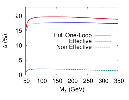
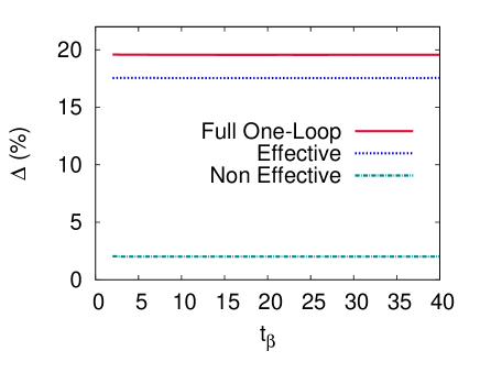
Figure 3: Corrections to the tree-level cross-section for the process $\tilde{\chi}_{1}^{0}\tilde{\chi}_{1}^{0}\rightarrow\mu^{+}\mu^{-}$ in the bino case as a function of $M_{1}$ (left panel) and $t_{\beta}$ right panel. We show the full one-loop, the effective correction and the difference which we term non effective. $M_{2}=500,\mu=-600\ GeV$.

The annihilation of neutralinos and hence the relic density is a very good example of the non decoupling effects of very heavy sparticles, a remnant of supersymmetry breaking. The variation in the fermion/sfermion masses is all contained in the effective couplings that we have introduced. Leaving the dependence on the smuon mass at tree-level, and the very small (see below) contribution of the smuon to the 1-PI vertex ${\tilde{\chi}}_{1}^{0}\mu\tilde{\mu}$, the bulk of the smuon mass dependence is within the effective coupling. Fig. 4 shows how the correction increases as the mass of the squarks increases from $400\ GeV$ to $3\ TeV$, we take here a common mass for the supersymmetry breaking squark masses (both right and left in all three generations). The non universal correction of about $2\%$ is insensitive to this change in squark masses whereas both $\Delta_{\rm eff}$ and $\Delta_{NU}$ show the same logarithm growth that brings a $3\%$ change as the squark mass is varied in the range $400\ GeV$ to $3\ TeV$.

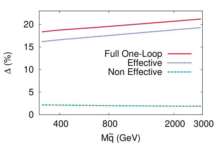
Figure 4: Corrections to the tree-level cross-section for the process $\tilde{\chi}_{1}^{0}\tilde{\chi}_{1}^{0}\rightarrow\mu^{+}\mu^{-}$ in the bino case ($M_{1}=90,M_{2}=200,\mu=-600\ GeV$) as function of the common soft supersymmetry breaking squark mass.

This result also confirms that genuine vertex corrections and box corrections are very small.
We have also extracted the individual contribution of each species of fermions to the total non-decoupling effect of sfermions. To achieve this we numerically extracted the logarithm dependence of the non decoupling effect for each species of sfermions. We have parameterised the effective correction as

$$\Delta^{f}=a_{\tilde{f}}\ln m_{\tilde{f}}/Q-a_{f}\ln m_{f}/Q+b_{f}\quad{\rm with}\quad Q=2m_{{\tilde{\chi}}_{1}^{0}}\quad\tilde{f}=\tilde{d}_{R}+\tilde{u}_{R}+\tilde{Q}_{L}$$ (18)

The coefficients of the fit are given in Table 1. As expected the fit to $a_{f}$ is extremely well reproduced by the running of $\alpha$, i.e, $a_{f}=N_{c}q_{f}^{2}\frac{4\alpha}{3\pi}$. We also find $a_{\tilde{e}}=a_{\tilde{\tau}}=a_{\tilde{\mu}},b_{e}=b_{\mu}=b_{\tau}$. The fit to $a_{f}$ is made to validate the fit procedure.

$$\begin{array}[]{|c|c|c|c|c|c|}\cline{2-6}\cr\lx@intercol\hfil\hfil\lx@intercol\vrule\lx@intercol&a_{\tilde{Q}_{L}}&a_{\tilde{u}_{R}}&a_{\tilde{d}_{R}}&a_{f}&b_{f}\\ \hline\cr e&0.0010&-&0.00231&0.00310&0.15\%\\ (u,d)&0.000575&0.00236&0.000698&(0.00413,0.00103)&0.15\%\\ (t,b)&-0.00406&0.00838&0.000661&(0.00413,0.00103)&0.16\%\\ \hline\cr\end{array}$$

Table 1: Coefficients of the $\ln(m_{f})$ (running couplings) $\ln(m_{\tilde{f}})$(non decoupling effects) in $\Delta_{\rm eff}$. $(c,s)$ give very similar results to $(u,d)$.

The most important observation is that the stops behave differently, this is due to the Yukawa coupling of the top and mixing. If there were not a compensation between left and right contribution of the stops (compare to $\tilde{u}$) the contribution of the stops would be even more important and would dominate. Considering the different contributions and the scales that enter our calculations it is difficult to attempt at giving an analytical result, but leaving the stop aside the different contributions to $a_{\tilde{f}}$ can be roughly approximated by $y_{f}^{2}N_{c}N_{d}/8/c_{W}^{2}$, $N_{d}=2$ for doublets and $1$ for singlet of $SU(2)$. $y_{f}$ is the hypercharge, corresponding to the couplings of the sfermions to the bino component.

3.1.2 Scheme dependence in the bino case

We have compared the full correction to an approximate effective implementation and observed that the approximation is quite good. However, even the full correction, being computed at one-loop, it is potentially dependent on the renormalisation scheme chosen. As discussed earlier we analyse the $t_{\beta}$ scheme dependence and the $M_{1}$ scheme dependence. For $t_{\beta}$ we obtain the following corrections:

$$19.58\%(DCPR),\quad 19.79\%(\overline{DR}),\quad 19.51\%(MH).$$

This confirms that the $t_{\beta}$ scheme dependence is very negligible. For the bino case it is natural to reconstruct $M_{1}$ from the LSP, nonetheless analysing the $M_{1}$ scheme dependence one chooses another neutralino, say ${\tilde{\chi}}_{2}^{0}$ which in our example is a wino-like. This introduces more uncertainty or error since with this scheme the corrections attain $24.08\%$, more than $4\%$ compared to the usual scheme.

3.2 Higgsino Case

3.2.1 Effective versus full corrections

In the bino case our trial point had a neutralino of mass $91\ GeV$. We therefore take the point (600,500,-100) which gives a LSP with $M_{\tilde{\chi}_{1}^{0}}=95\ GeV$ with a 99% higgsino content. The sfermion parameters are the default values. In the higgsino case the cross section is dominated by the exchange of the $Z$ in the $s$-channel, so the bulk of the corrections through the effective couplings will be through the effective ${\tilde{\chi}}_{1}^{0}{\tilde{\chi}}_{1}^{0}Z$. For further reference note that the tree-level cross section for annihilation into muons is $\sigma_{\mu^{+}\mu^{-}}^{\tilde{h}}=2.58\times 10^{-3}{\rm pb}$, tiny and totally insignificant especially compared to annihilation into $W$, $\sigma_{W^{+}W^{-}}^{\tilde{h}}=18.83\ {\rm pb}$. This is an observation we will keep in mind. The one-loop corrections we find for $\sigma_{\mu^{+}\mu^{-}}^{\tilde{h}}$ are

$$({\rm for}\;\mu=-100{\rm GeV})\quad\quad\Delta_{\rm eff}=13.55(\Delta_{\alpha}=14.62\%)\quad\Delta_{NU}=-21.09\%(\Delta_{full}=-7.54\%)$$ (19)

This result is in a quite striking contrast to the bino case. The effective coupling does not reproduce at all the full correction and is off by as much as $21\%$. It looks like, at least for this particular choice of parameters, that going through the trouble of implementing the effective ${\tilde{\chi}}_{1}^{0}{\tilde{\chi}}_{1}^{0}Z$ was in vain since this correction is, within a per-cent, reproduced by the naive running of $\alpha$. As we will see both these conclusions depend much on the parameters of the higgsino and even the squark masses. For example consider $\mu=-50\ GeV$, leaving all other parameters the same. Of course this is a purely academic exercise, since in this case, the charginos with mass $m_{\chi^{\pm}_{1}}=55\ GeV$ are ruled out by LEP data. Nonetheless, in this case

$$({\rm for}\;\mu=-50{\rm GeV})\quad\quad\Delta_{\rm eff}=10.7(\Delta_{\alpha}=12\%)\quad\Delta_{NU}=-6.9\%(\Delta_{full}=3.8\%).$$ (20)

Had we included all particles in the effective vertex, we would get a correction $\Delta_{\rm eff}^{W}=4.4\%$ improving thus the agreement with the one-loop correction for this particular value of $\mu$ up to $0.6\%$. At the same time a correction in terms of a running of $\alpha$ will be off by more than 8%.

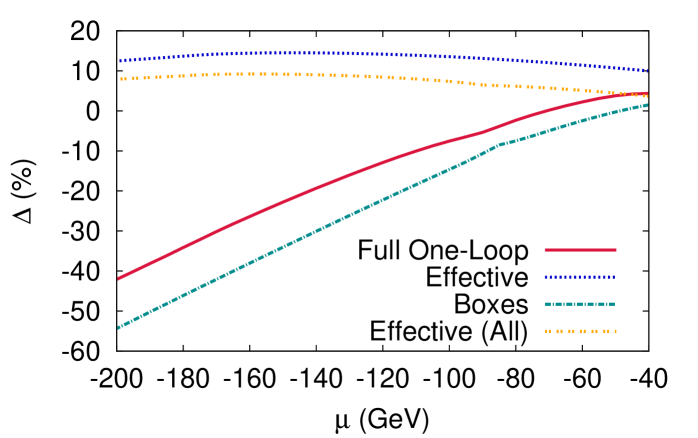
Figure 5: Corrections to the tree-level cross-section for the process $\tilde{\chi}_{1}^{0}\tilde{\chi}_{1}^{0}\rightarrow\mu^{+}\mu^{-}$ in the higgsino case as a function of $\mu$. Shown are the effective vertex correction (Effective, with only fermions/sfermions in the loops), the effective ${\tilde{\chi}}_{1}^{0}{\tilde{\chi}}_{1}^{0}Z$ coupling including all particles denoted Effective (All), the non QED boxes (Boxes) and the full correction. $M_{2}=500,\mu=-600\ GeV$.

These two examples show that one can not, in the higgsino case, draw a general conclusion on the efficiency of the effective coupling as what was done in the bino case. Let us therefore look at how the corrections change with $\mu$, and therefore with the mass of the LSP, while maintaining its higgsino nature. We have varied $\mu$ from $-200\ GeV$ to $-40\ GeV$. Fig. 5 shows that the full correction is extremely sensitive to the value of $\mu$. For $\mu=-200\ GeV$ the full one-loop correction is much as $-42\%$, casting doubt on the loop expansion. The effective coupling corrections with only fermions/sfermions on the other hand is much smoother and positive bringing about $10\%$ correction. Including all particles in the effective ${\tilde{\chi}}_{1}^{0}{\tilde{\chi}}_{1}^{0}Z$ vertex brings in an almost constant reduction of about $6\%$. Therefore as the value of $|\mu|$ increases the effective one-loop corrections in the case of the higgsino case can not be trusted. The same figure shows that the behaviour and the increase in the corrections is due essentially to the contribution of the boxes. Here the boxes mean the non QED box (involving an exchange of a photon which are infrared divergent before including the real photon emission). The large contribution of the boxes can be understood by looking at the box in Fig. 1(c). Indeed, as argued previously, cutting through the box reveals that it represents ${\tilde{\chi}}_{1}^{0}{\tilde{\chi}}_{1}^{0}\to W^{+}W^{-}$ production that rescatter into $\mu^{+}\mu^{-}$. Both these process have a very large cross sections compared to the tree-level ${\tilde{\chi}}_{1}^{0}{\tilde{\chi}}_{1}^{0}\to\mu^{+}\mu^{-}$. Our conclusion is therefore that the effective vertex approximation is inadequate as soon as the channel ${\tilde{\chi}}_{1}^{0}{\tilde{\chi}}_{1}^{0}\to W^{+}W^{-}$ opens up. When this occurs, in practical calculations of the relic density, the channel ${\tilde{\chi}}_{1}^{0}{\tilde{\chi}}_{1}^{0}\to\mu^{+}\mu^{-}$ is irrelevant and must rather analyse the loop corrections to ${\tilde{\chi}}_{1}^{0}{\tilde{\chi}}_{1}^{0}\to W^{+}W^{-}$. This process was studied in[13, 10] and will be investigated further through an effective approximation in a forthcoming study.
On the other hand, the dependence of the relative correction on $t_{\beta}$ is quite modest even though there is certainly more dependence than in the bino case, especially at lower values of $\tan\beta$. This is shown in Fig. 6.

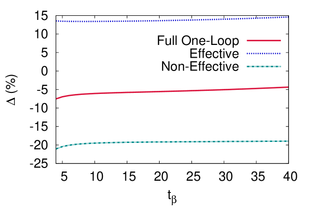
Figure 6: Corrections to the tree-level cross-section for the process $\tilde{\chi}_{1}^{0}\tilde{\chi}_{1}^{0}\rightarrow\mu^{+}\mu^{-}$ in the higgsino case as a function of $t_{\beta}$. We show the full one-loop, the effective correction and the remainder (Non-effective). $\mu=-100,M_{2}=500,\mu=-600\ GeV$.

We now investigate the non-decoupling of very heavy squarks (and heavy sfermions in general). Since we are in a Higgsino scenario we expect the Yukawa of the fermions to play a more prominent role than what was observed in the bino case. This is well supported by our study. Fig. 7 shows how the effective (with only fermions and sfermions) and the full correction gets modified when the common mass of all squarks (all generations, left and right) increases from $400\ GeV$ to $3\ TeV$. To better illustrate the important effect of the Yukawa of the top/stop sector we plot the corrections also for $m_{t}=0.1\ GeV$. For $m_{t}=170.9\ GeV$, the correction drops by about $13\%$ when the mass of the squarks increase from $400\ GeV$ to $3\ TeV$. This is much more dramatic than in the bino case where we observed a 3% increase in the same range. Observe that for our default squark mass of $800\ GeV$, the effective correction including sfermions/fermions is such that it almost accidently coincides with the running of $\alpha$. If one switches off the top quark mass, instead of a 13% decrease we observe an 8% increase for $m_{t}=0.1\ GeV$! Observe that the difference one sees for $m_{\tilde{Q}}=400\ GeV$ between $m_{t}=170.9\ GeV$ and $m_{t}=0.1\ GeV$ is due essentially to the running of $\alpha$ with very light top that accounts for $3\%$.

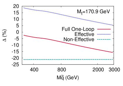
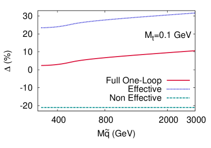
Figure 7: Corrections to the tree-level cross-section for the process $\tilde{\chi}_{1}^{0}\tilde{\chi}_{1}^{0}\to\mu^{+}\mu^{-}$ in the higgsino case ($M_{1}=600,M_{2}=500,\mu=-100$) as function of the common squark mass. The right panel illustrates the case $m_{t}=0.1\ GeV$.

The special role played by the top can be seen even more clearly from each individual contribution of the fermion/sfermions and the fit of the contribution according to Eq. 18 as was done for the bino case.

$$\begin{array}[]{|c|c|c|c|c|c|}\cline{2-6}\cr\lx@intercol\hfil\hfil\lx@intercol\vrule\lx@intercol&a_{\tilde{Q}_{L}}&a_{\tilde{u}_{R}}&a_{\tilde{d}_{R}}&a_{f}&b_{f}\\ \hline\cr e&0.00304&-&0.000366&0.00309&-0.12\%\\ (u,d)&0.00861&0.000489&0.000122&(0.00414,0.00101)&-0.13\%\\ (t,b)&-0.0701&0.000826&0.000108&(0.00414,0.00101)&0.13\%\\ \hline\cr\end{array}$$

Table 2: Coefficients of the $\ln(m_{f})$ (running couplings) $\ln(m_{\tilde{f}})$(non decoupling effects) in $\Delta_{\rm eff}$. $(c,s)$ give very similar results to $(u,d)$. Higgsino case.

The contribution of the stop is clearly (especially through $\tilde{Q}_{L}$) an order of magnitude larger than for all other sfermions, see Table 2. It is the only one that brings a negative contribution. Since this effect is in the universal ${\tilde{\chi}}_{1}^{0}{\tilde{\chi}}_{1}^{0}Z$ it will show up in many processes where the higgsino contributes.

3.2.2 Scheme dependence in the higgsino case

We analyse here the $t_{\beta}$ scheme dependence and the $M_{1}$ scheme dependence. For $t_{\beta}$ we obtain the following corrections:

$$-7.5\%(DCPR),\quad-12.4\%(\overline{DR}),\quad-4.76\%(MH).$$

As expected and in line with the behaviour of the corrections with respect to $\tan\beta$, Fig. 6, we see that the corrections though larger than in the bino case are nonetheless within 5%. On the other hand, expectedly the choice of $M_{1}$ has less impact than in the bino case where the reconstruction of $M_{1}$ is essential to define the LSP. In the case of the higgsino, changing the $M_{1}$ scheme turns the full correction from -7.5% (in DCPR scheme for $t_{\beta}$) to -10.7%, a 3% uncertainty.

4 Conclusions

Very few analyses have been done taking into account the full one-loop corrections to the annihilation cross sections entering the computation of the relic density despite the fact that this observable is now measured within 3% precision. In supersymmetry radiative corrections have been known to be important, yet practically all analyses that constrain the parameter space of supersymmetry are performed with tree-level annihilation cross sections. Taking into account the full one-loop corrections to a plethora of processes is most probably unrealistic. On the other hand one must incorporate, if possible simply and quickly, a parameterisation of the theory error or implement the corrections through effective couplings of the neutralino, in the case of supersymmetry. This is what we have attempted in this study for two of the most important couplings of the neutralinos ${\tilde{\chi}}_{1}^{0}f\tilde{f}$ and ${\tilde{\chi}}_{1}^{0}{\tilde{\chi}}_{1}^{0}Z$. In order to look more precisely at the impact of each of these effective couplings we take as a testing ground a most simple process, ${\tilde{\chi}}_{1}^{0}{\tilde{\chi}}_{1}^{0}\to\mu^{+}\mu^{-}$ and select a neutralino that is either almost pure bino or pure higgsino. We do not strive at finding a scenario with the correct relic density since our primary task is to study this vertices and the approximations in detail. In this exploratory study taking a final state involving gauge bosons would only confuse the issues. Nonetheless, the impact of the gauge bosons is studied. Indeed, we have shown how the construction of the effective ${\tilde{\chi}}_{1}^{0}{\tilde{\chi}}_{1}^{0}Z$ is quite different from that of the ${\tilde{\chi}}_{1}^{0}f\tilde{f}$. For the latter the effective coupling involves self-energy corrections, whereas for the former the one-particle irreducible vertex correction must be added. These examples and the construction of the effective coupling already pave the way to a generalisation to the effective couplings ${\tilde{\chi}}_{1}^{0}{\tilde{\chi}}_{1}^{0}h,H,A$ and ${\tilde{\chi}}_{1}^{0}\chi^{+}W$ which we will address in forthcoming publications with applications to different process, including gauge boson final states. Even with the effective couplings we have derived, we could generalise the study of ${\tilde{\chi}}_{1}^{0}{\tilde{\chi}}_{1}^{0}\to\mu^{+}\mu^{-}$ to cover not only pure winos, but also mixed scenarios and also heavy fermions.
Our preliminary study on the simple process ${\tilde{\chi}}_{1}^{0}{\tilde{\chi}}_{1}^{0}\to\mu^{+}\mu^{-}$ is already very instructive. To summarise the bino case, we can state that the effective couplings approach is a very good approximation that embodies extremely well the non decoupling effects from heavy sfermions, irrespective of many of the parameters that are involved in the calculation, as long as one is in an almost pure bino case. The effective coupling implementation is within $2\%$ of the full one-loop calculation. Here, this reflects essentially the correction to the ${\tilde{\chi}}_{1}^{0}f\tilde{f}$ coupling. The scheme dependence from $t_{\beta}$ is very small, this result stands for large $M_{1}$ masses as long as the neutralino is more than $90\%$ bino like. In particular for higgsino-like LSP in excess of $90\ GeV$ as imposed by present limits on the chargino, the effective coupling implementation in the annihilation ${\tilde{\chi}}_{1}^{0}{\tilde{\chi}}_{1}^{0}\to\mu^{+}\mu^{-}$ fails. It worsens as the mass increases due to the importance of a large box contribution corresponding to the opening up of ${\tilde{\chi}}_{1}^{0}{\tilde{\chi}}_{1}^{0}\to W^{+}W^{-}$ which would in any case be the dominant process to take into account when calculating the relic density. The large Yukawa of the top has a big impact on the radiative corrections and in particular on the non-decoupling contribution of a very heavy stop. Although this is an example which shows, in principle, the failure of the effective approach apart from correctly reproducing the non-decoupling effect of very heavy squarks, we need further investigation on the dominant processes, in this case annihilations into $W,Z$, to see if these dominant processes could on the other hand be reproduced by an effective coupling approach. If the effective approach turns out to be efficient for the dominant processes, where and if the box corrections are tamed, the effective coupling could still be a good alternative for the calculation of the relic density with high precision. We leave many of these interesting issues to further analyses.

Acknowledgments
We would like to thank Guillaume Chalons for many useful discussions. This work is part of the French ANR project, ToolsDMColl BLAN07-2 194882 and is supported in part by the GDRI-ACPP of the CNRS (France). GDLR held a fellowship from la Région Rhones-Alpes. This work was supported by TRR33 ”The Dark Universe”.

References

-
[1]
see for example, S. Caron for the ATLAS collaboration, arXiv:1106.1009
[hep-ex].
J. B. G. da Costa et al. [Atlas Collaboration], Phys. Lett. B 701 (2011) 186 [arXiv:1102.5290 [hep-ex]].
G. Aad et al. [ATLAS Collaboration], Eur. Phys. J. C 71 (2011) 1682 [arXiv:1103.6214 [hep-ex]].
S. Chatrchyan et al. [ CMS Collaboration ],[arXiv:1107.1279 [hep-ex]]. - [2] See for example, W. Murray, Higgs searches at the LHC, Plenary Summary talk at the Europhysics Conference on High-Energy Physics, Grenoble (2011).
- [3] N. Jarosik et al., Astrophys. J. Suppl. 192 (2011) 14 [arXiv:1001.4744 [astro-ph.CO]].
- [4] B. A. Reid et al. [SDSS Collaboration], Mon. Not. Roy. Astron. Soc. 401 (2010) 2148 [arXiv:0907.1660 [astro-ph.CO]].
- [5] A. G. Riess et al., Astrophys. J. 699 (2009) 539 [arXiv:0905.0695 [astro-ph.CO]].
- [6] E. Komatsu et al. [WMAP Collaboration], Astrophys. J. Suppl. 192 (2011) 18 [arXiv:1001.4538 [astro-ph.CO]].
-
[7]
G. Bélanger, F. Boudjema, A. Pukhov, A. Semenov, Comput. Phys.
Commun. 149 (2002) 103, hep-ph/0112278;
G. Bélanger, F. Boudjema, A. Pukhov, A. Semenov, Comput. Phys. Commun. 176 (2007) 367, hep-ph/0607059;
G. Bélanger, F. Boudjema, A. Pukhov, A. Semenov, Comput. Phys. Commun. 174 (2006) 577, hep-ph/0405253;
http://lapth.in2p3.fr/micromegas. -
[8]
DarkSUSY: P. Gondolo et al., JCAP 0407 (2004)
008, astro-ph/0406204;
http://www.physto.se/edsjo/darksusy/. -
[9]
SuperIso Relic: A. Arbey, F. Mahmoudi, A. Arbey and F. Mahmoudi, Comput. Phys. Commun. 181 (2010) 1277 [arXiv:0906.0369 [hep-ph]].
Comput. Phys. Commun. 182, 1582 (2011).
http://superiso.in2p3.fr/relic/. - [10] N. Baro, F. Boudjema, A. Semenov, Phys. Lett. B660 (2008) 550, arXiv:0710.1821 [hep-ph].
- [11] A. Freitas, Phys. Lett. B 652 (2007) 280 [arXiv:0705.4027 [hep-ph]].
-
[12]
B. Herrmann, M. Klasen, Phys. Rev. D76 (2007) 117704,
arXiv:0709.2232 [hep-ph].
B. Herrmann, M. Klasen, K. Kovarik, Phys. Rev. D79 (2009) 061701, arXiv:0901.0481 [hep-ph].
B. Herrmann, M. Klasen, K. Kovarik, Phys. Rev. D80 (2009) 085025, arXiv:0907.0030[hep-ph]. - [13] N. Baro, F. Boudjema, G. Chalons and S. Hao, Phys. Rev. D 81 (2010) 015005 [arXiv:0910.3293 [hep-ph]].
- [14] For a recent review, see B. Herrmann, arXiv:1011.6550 [hep-ph].
- [15] F. Boudjema, J. Edsjo and P. Gondolo, in Particle dark matter 325-344, Oxford University Press (2010) G. Bertone, editor; Matter and at the Colliders,” [arXiv:1003.4748 [hep-ph]].
- [16] H. C. Cheng, J. L. Feng and N. Polonsky, Phys. Rev. D 56 (1997) 6875, [arXiv:hep-ph/9706438]; idem Phys. Rev. D 57 (1998) 152, [arXiv:hep-ph/9706476].
- [17] E. Katz, L. Randall and S. f. Su, Nucl. Phys. B 536 (1998) 3 [arXiv:hep-ph/9801416].
- [18] S. Kiyoura, M. M. Nojiri, D. M. Pierce and Y. Yamada, Phys. Rev. D 58, 075002 (1998) [arXiv:hep-ph/9803210].
- [19] For a recent review see, A. Hryczuk, Phys. Lett. B 699 (2011) 271 [arXiv:1102.4295 [hep-ph]].
-
[20]
L. J. Hall, R. Rattazzi and U. Sarid, Phys. Rev. D 50 (1994) 7048
[arXiv:hep-ph/9306309].
M. S. Carena, M. Olechowski, S. Pokorski and C. E. M. Wagner, Nucl. Phys. B 426 (1994) 269 [arXiv:hep-ph/9402253].
M. S. Carena, D. Garcia, U. Nierste and C. E. M. Wagner, Nucl. Phys. B 577 (2000) 88 [arXiv:hep-ph/9912516]. -
[21]
P. Salati, Phys. Lett. B 571 (2003) 121 [arXiv:astro-ph/0207396].
S. Profumo and P. Ullio, JCAP 0311 (2003) 006 [arXiv:hep-ph/0309220].
F. Rosati, Phys. Lett. B 570 (2003) 5 [arXiv:hep-ph/0302159].
C. Pallis, JCAP 0510 (2005) 015 [arXiv:hep-ph/0503080].
G. B. Gelmini and P. Gondolo, Phys. Rev. D74 (2006) 023510 [arXiv:hep-ph/0602230].
D. J. H. Chung, L. L. Everett, K. Kong and K. T. Matchev, arXiv:0706.2375 [hep-ph].
M. Drees, H. Iminniyaz and M. Kakizaki, Phys.Rev. D76 (2007) 103524, [arXiv:0704.1590[hep-ph]].
A. Arbey and F. Mahmoudi, JHEP 1005 (2010) 051 [arXiv:0906.0368 [hep-ph]]. -
[22]
A. Semenov. LanHEP — a package for automatic generation of Feynman
rules. User’s manual.; hep-ph/9608488.
A. Semenov, Nucl. Inst. Meth. and Inst. A393 (1997) 293;
A. Semenov, Comp. Phys. Commun. 115 (1998) 124;
A. Semenov, hep-ph/0208011;
A. Semenov, Comput. Phys. Commun. 180 (2009) 431, arXiv:0805.0555 [hep-ph]. -
[23]
J. Küblbeck, M. Böhm, A. Denner, Comp. Phys. Commun. 60
(1990) 165;
H. Eck, J. Küblbeck, Guide to FeynArts 1.0, Würzburg, 1991;
H. Eck, Guide to FeynArts 2.0, Würzburg, 1995;
T. Hahn, Comp. Phys. Commun. 140 (2001) 418, hep-ph/0012260. -
[24]
T. Hahn, M. Perez-Victoria, Comp. Phys. Commun. 118 (1999) 153,
hep-ph/9807565;
T. Hahn, hep-ph/0406288; hep-ph/0506201. -
[25]
T. Hahn, LoopTools,
http://www.feynarts.de/looptools/. - [26] F. Boudjema, A. Semenov, D. Temes, Phys. Rev. D72 (2005) 055024, hep-ph/0507127.
- [27] N. Baro, F. Boudjema, A. Semenov, Phys. Rev. D78 (2008) 115003, arXiv:0807.4668 [hep-ph].
- [28] N. Baro, F. Boudjema, Phys. Rev D80 (2009) 076010, [arXiv:0906.1665 [hep-ph]].
- [29] G. Bélanger, F. Boudjema, J. Fujimoto, T. Ishikawa, T. Kaneko, K. Kato, Y. Shimizu, Phys. Rep. 430 (2006) 117, hep-ph/0308080.
- [30] G. Bélanger, F. Boudjema, J. Fujimoto, T. Ishikawa, T. Kaneko, K. Kato and Y. Shimizu, Phys. Lett. B559 (2003) 252; hep-ph/0212261.
- [31] A. Dabelstein, Z. Phys. C67 (1995) 495, hep-ph/9409375.
- [32] P.H. Chankowski, S. Pokorski and J. Rosiek, Nucl. Phys. B423 (1994) 437, hep-ph/9303309.
-
[33]
D.Z. Freedman, K. Johnson, J.I. Latorre, Nucl. Phys. B371 (1992)
353;
P.E. Haagensen, Mod. Phys. Lett. A7 (1992) 893, hep-th/9111015;
F. del Aguila, A. Culatti, R. Muñoz Tapia, M. Pérez-Victoria, Phys. Lett. B419 (1998) 263, hep-th/9709067;
F. del Aguila, A. Culatti, R. Muñoz Tapia, M. Pérez-Victoria, Nucl. Phys. B537 (1999) 561, hep-ph/9806451;
F. del Aguila, A. Culatti, R. Muñoz Tapia, M. Pérez-Victoria, Nucl. Phys. B504 (1997) 532, hep-ph/9702342. - [34] J. Guasch, W. Hollik and J. Sola, JHEP 0210, 040 (2002) [arXiv:hep-ph/0207364].