Electron-phonon-scattering dynamics in ferromagnetic metals and its influence on ultrafast demagnetization processes

Abstract

We theoretically investigate spin-dependent carrier dynamics due to the electron-phonon interaction after ultrafast optical excitation in ferromagnetic metals. We calculate the electron-phonon matrix elements including the spin-orbit interaction in the electronic wave functions and the interaction potential. Using the matrix elements in Boltzmann scattering integrals, the momentum-resolved carrier distributions are obtained by solving their equation of motion numerically. We find that the optical excitation with realistic laser intensities alone leads to a negligible magnetization change, and that the demagnetization due to electron-phonon interaction is mostly due to hole scattering. Importantly, the calculated demagnetization quenching due to this Elliot-Yafet type depolarization mechanism is not large enough to explain the experimentally observed result. We argue that the ultrafast demagnetization of ferromagnets does not occur exclusively via an Elliott-Yafet type process, i.e., scattering in the presence of the spin-orbit interaction, but is influenced to a large degree by a dynamical change of the band structure, i.e., the exchange splitting.

I Introduction

It was first demonstrated more than ten years ago that the magnetization of ferromagnets can be “quenched” on ultrashort time scales after ultrafast optical excitation. Beaurepaire et al. (1996) Apart from the possibilities for the ultrafast manipulation of ferromagnetism in applications, this observation raised the question how demagnetization dynamics in ferromagnets on a time scale of a few hundred femtoseconds can be understood.

Aside from the phenomenological three-temperature model, Beaurepaire et al. (1996); Koopmans et al. (2010) which leads to quite successful comparison with experiment, there are several theoretical models and experimental results that try to explain aspects of the underlying microscopic dynamics. For instance, the analysis of X-ray magnetic circular dichroism measurements suggested that the orbital magnetic moment does not play a prominent role in the demagnetization dynamics. Stamm et al. (2007); Carva et al. (2009) The authors of Ref. Stamm et al., 2007 concluded that an ultrafast spin-lattice coupling should be operative to explain the results. It has also been argued based on experimental results Carpene et al. (2008) that the excitation of magnons should play an important role. On the theory side, magnetic switching due to electronic transitions during the duration of a pump laser pulse has been analyzed in ferromagnets Zhang and Hübner (2000); Zhang et al. (2009) as well as in oxides (including phonons), Lefkidis and Hübner (2009) and the Landau-Lifshitz-Bloch equations have been used to describe the magnetic dynamics. Atxitia et al. (2010)

Perhaps the most popular microscopic explanations of the effect involve variations of the so-called Elliott-Yafet mechanism, in which demagnetization (or depolarization in semiconductors) is due to incoherent scattering of carriers between states that are spin-mixed due to the spin-orbit interaction. Electron-electron scattering is a possible candidate as the underlying scattering mechanism, Krauß et al. (2009) but the focus is usually on the effects of electron-phonon scattering in quasi-equilibrium. Koopmans et al. (2005); Walowski et al. (2008); Steiauf and Fähnle (2009); Steiauf et al. (2010) In addition, superdiffusive transport processes can contribute to the measured Kerr-effect signal because minority and majority electrons may simply leave the probe area at different speeds. Battiato et al. (2010)

In our opinion, it has so far been impossible rule out a single one of these mechanisms, let alone to pinpoint the dominant one. As a first step in this direction, we analyze a parameter-free microscopic model for ultrafast demagnetization and compare it with experiment. To keep things simple while allowing a conclusive statement, we exclusively treat the effect of the optical excitation and electron-phonon scattering at the level of Boltzmann scattering integrals while neglecting dynamical changes in the band structure, i.e., the exchange splitting, in the course of the dynamics. We evaluate the model using ab-initio results for the simple ferromagnets nickel and iron. Comparison of the results of the present paper with experimental data, which are available from many different measurements, will show that a model without band structure changes yields a demagnetization that is too small.

This paper is organized as follows. In Sec. II we present the dynamical equations for the carrier distribution functions and show how we calculate the electron-phonon and dipole matrix elements using a first-principles approach. In Sec. III we discuss the numerical results of this model and show that the demagnetization using realistic parameters for the ultrashort-pulse excitation is due to hole dynamics, but too small to agree with experiment. A qualitative consideration shows that this conclusion should not be altered by including additional scattering processes. Sec. IV contains the conclusions and the Appendix describes details of our numerical evaluation of the dynamical equations.

II Theory

II.1 Dynamical equations

The basic idea of this paper is to integrate the dynamical equations of motions for the band- and momentum-resolved carrier distributions $n_{\vec{k}}^{\mu}(t)$. Our model includes the incoherent scattering dynamics due to the electron-phonon interaction, as well as the optical excitation, so that the general form of the dynamical equation is

$$\frac{\partial}{\partial t}n_{\vec{k}}^{\mu}=\frac{\partial}{\partial t}n_{\vec{k}}^{\mu}\Bigr{|}_{\text{opt}}+\frac{\partial}{\partial t}n_{\vec{k}}^{\mu}\Bigr{|}_{\text{e-p}}.$$ (1)

The optical excitation is given by

$$\frac{\partial}{\partial t}n_{\vec{k}}^{\mu}\Bigr{|}_{\text{opt}}=\frac{2\pi}{\hbar}\sum_{\nu(\neq\mu)}\bigl{|}\vec{d}_{\vec{k}}^{\mu\nu}\cdot\vec{E}(t)\bigr{|}^{2}g(\epsilon_{\vec{k}}^{\mu}-\epsilon_{\vec{k}}^{\nu}-\hbar\omega_{L})\bigl{[}n_{\vec{k}}^{\nu}-n_{\vec{k}}^{\mu}\bigr{]}.$$ (2)

Here, $\epsilon_{\vec{k}}^{\mu}$ is the energy of a carrier in a single-particle state $\psi_{\vec{k}}^{\mu}$ with band index $\mu$ and momentum $\vec{k}$. The dipole matrix element for a transition connecting two such states is denoted by $\vec{d}_{\vec{k}}^{\mu\nu}=\langle\psi_{\vec{k}}^{\mu}|\,e\vec{r}\,|\psi_{\vec{k}}^{\nu}\rangle$. The optical excitation is characterized by the dynamical electric field amplitude $\vec{E}(t)$, a central laser frequency $\omega_{\mathrm{L}}$, and the function $g(\epsilon)$ that includes the spectral profile of the laser pulse.

The electron-phonon contribution to the carrier dynamics at the level of Boltzmann scattering integrals reads

$$\frac{\partial}{\partial t}n_{\vec{k}}^{\mu}\Bigr{|}_{\text{e-p}}=\frac{2\pi}{\hbar}\sum_{\vec{k}^{\prime},\nu}\Bigl{[}w(\vec{k}^{\prime},\nu\rightarrow\vec{k},\mu)n_{\vec{k}^{\prime}}^{\nu}\bigl{(}1-n_{\vec{k}}^{\mu}\bigr{)}\\ -w(\vec{k},\mu\rightarrow\vec{k}^{\prime},\nu)n_{\vec{k}}^{\mu}\bigl{(}1-n_{\vec{k}^{\prime}}^{\nu}\bigr{)}\Bigr{]},$$ (3)

where the scattering rates $w(\vec{k}^{\prime},\nu\rightarrow\vec{k},\mu)$ from state $\psi_{\vec{k}^{\prime}}^{\nu}$ to $\psi_{\vec{k}}^{\mu}$

$$\begin{split}w(\vec{k}^{\prime},\nu\rightarrow\vec{k},\mu)=\sum_{\lambda}\Bigl{[}&\bigl{|}M_{+}^{\vec{k}-\vec{k}^{\prime},\lambda}(\vec{k}^{\prime},\nu\rightarrow\vec{k},\mu)\bigr{|}^{2}\tilde{n}_{\vec{k}-\vec{k}^{\prime}}^{\lambda}\,\delta(\epsilon_{\vec{k}^{\prime}}^{\nu}-\epsilon_{\vec{k}}^{\mu}+\hbar\omega_{\vec{k}-\vec{k}^{\prime}}^{\lambda})\\ +&\bigl{|}M_{-}^{\vec{k}^{\prime}-\vec{k},\lambda}(\vec{k}^{\prime},\nu\rightarrow\vec{k},\mu)\bigr{|}^{2}(\tilde{n}_{\vec{k}^{\prime}-\vec{k}}^{\lambda}+1)\,\delta(\epsilon_{\vec{k}^{\prime}}^{\nu}-\epsilon_{\vec{k}}^{\mu}-\hbar\omega_{\vec{k}^{\prime}-\vec{k}}^{\lambda})\Bigr{]}\end{split}$$ (4)

have contributions from absorption (“$+$”) and emission (“$-$”) processes. The (angular) frequency of a phonon mode $\lambda$ is designated by $\omega_{\vec{q}}^{\lambda}$ and its occupation at quasi-momentum $\vec{q}$ by $\tilde{n}_{\vec{q}}^{\lambda}$. The electron-phonon interaction matrix elements $M_{{\pm}}^{\vec{q},\lambda}(\vec{k}^{\prime},\nu\rightarrow\vec{k},\mu)$ result from the change of the electron-lattice interaction energy due to the vibrational motion of the nuclei. For small displacements they are given by

$$M_{{\pm}}^{\vec{q},\lambda}(\vec{k}^{\prime},\nu\rightarrow\vec{k},\mu)=\sqrt{\frac{\hbar}{2MN\omega_{\vec{q}}^{\lambda}}}\sum_{j}e^{\pm i\vec{q}\cdot\vec{R}_{j}}\Bigl{\langle}\psi_{\vec{k}}^{\mu}\Bigr{|}\vec{\pi}_{\vec{q}}^{\lambda}\cdot\frac{\partial}{\partial\vec{R}_{j}}V(\vec{r};\{\vec{R}_{i}\})\Bigl{|}\psi_{\vec{k}^{\prime}}^{\nu}\Bigr{\rangle}.$$ (5)

The electron-lattice interaction potential $V(\vec{r};\{\vec{R}_{i}\})$ depends on the electron position $\vec{r}$ and, in principle, on the set of the positions of the nuclei $\{\vec{R}_{i}\}$ in the crystal composed of $N$ unit cells with atomic mass $M$. The polarization vector of the phonon mode $(\vec{q},\lambda)$ is denoted by $\vec{\pi}_{\vec{q}}^{\lambda}$. The upper and lower signs in the exponential are associated with the phonon absorption $M_{+}^{\vec{q},\lambda}(\vec{k}^{\prime},\nu\rightarrow\vec{k},\mu)$ and emission $M_{-}^{\vec{q},\lambda}(\vec{k}^{\prime},\nu\rightarrow\vec{k},\mu)$ matrix elements, respectively.

In our calculation, we assume that the phonon occupation numbers are time independent and remain at their equilibrium values

$$\tilde{n}_{\vec{q}}^{\lambda}=\frac{1}{e^{\hbar\omega_{\vec{q}}^{\lambda}/k_{B}T_{0}}-1}.$$ (6)

This amounts to a bath assumption for the phonon system, and in this paper we fix its temperature at $T_{0}=300$ K, i.e., the temperature of the unexcited system in most studies of demagnetization dynamics.

From the dynamical electronic occupation numbers calculated according to Eq. (1), we obtain the time-dependent magnetization by

$$M(t)=\frac{2\mu_{B}}{\hbar}\sum_{\vec{k}}\sum_{\mu}\left\langle S_{z}\right\rangle_{\vec{k}}^{\mu}n_{\vec{k}}^{\mu}(t),$$ (7)

with the single-particle spin expectation value

$$\left\langle S_{z}\right\rangle_{\vec{k}}^{\mu}=\bigl{\langle}\psi_{\vec{k}}^{\mu}\bigr{|}\hat{S}_{z}\bigl{|}\psi_{\vec{k}}^{\mu}\bigr{\rangle}$$ (8)

in the Bloch state $\bigl{|}\psi_{\vec{k}}^{\mu}\bigr{\rangle}$ and the Bohr magneton $\mu_{B}$. In writing these relations, we have chosen the $z$-direction as direction of the ferromagnetic polarization. Orbital angular-momentum contributions to the magnetization are neglected as their influence on the magnetization of elementary ferromagnets is small.

II.2 Electron-phonon matrix elements

The numerical evaluation of Eq. (1) requires as input material properties, in particular, the electronic band structure $\epsilon_{\vec{k}}^{\mu}$, the spin expectation value of the single-particle states $\langle S_{z}\rangle_{\vec{k}}^{\mu}$, the dipole transition matrix elements $\vec{d}_{\vec{k}}^{\mu\nu}$, the phonon dispersion $\omega_{\vec{q}}^{\lambda}$, and, importantly, the electron-phonon matrix elements $M_{{\pm}}^{\vec{q},\lambda}(\vec{k}^{\prime},\nu\rightarrow\vec{k},\mu)$. We obtain these quantities from density-functional theory to avoid the introduction of adjustable parameters. To this end, we employ the augmented spherical wave (ASW) method Williams et al. (1979) as described in the monograph Ref. Kübler, 2000 (see also Ref. Eyert, 2007). The implementation of the ASW method used by us was developed in the Kübler group and relies on the scalar relativistic and local spin-density approximations. It includes spin-orbit coupling in a second variational correction.

The starting point for the calculation of the matrix elements is the representation of the wave function of a single-particle state with band index $\mu$ and momentum $\vec{k}$ in the ASW basis. Since we employ the atomic sphere approximation (ASA) it is usually sufficient to know the wave functions inside the atomic spheres where they are given by

$$\psi_{\vec{k}}^{\mu}(\vec{r})=\sum_{L,\sigma}\bigl{[}C_{L\sigma}^{\mu}(\vec{k})i^{l}\tilde{h}_{l\sigma}(r)+A_{L\sigma}^{\mu}(\vec{k})i^{l}\tilde{j}_{l\sigma}(r)\bigr{]}Y_{L}(\hat{r})\chi_{\sigma}$$ (9)

where $\tilde{h}_{l\sigma}(r)$ and $\tilde{j}_{l\sigma}(r)$ are augmented spherical waves, $Y_{L}(\hat{r})$ spherical harmonics, and $\chi_{\sigma}$ Pauli spinors. Here, $L=(l,m)$ is a multi-index that includes both the angular momentum and the magnetic quantum number. The relatively simple expression given here is only valid for materials with basis consisting of a single atom, such as the simple ferromagnets investigated in the present paper. The spherical wave functions, together with the coefficients $A_{L\sigma}^{\mu}(\vec{k})$ and $C_{L\sigma}^{\mu}(\vec{k})$, are calculated self-consistently during the iterative solution of the Kohn-Sham equations.

For the evaluation of Eq. (5), we employ the so-called rigid ion approximation. That is, we assume that we can write the lattice-configuration dependence of the electron-phonon interaction potential

$$V(\vec{r};\{\vec{R}_{i}\})=\sum_{i}v(\vec{r}-\vec{R}_{i})$$ (10)

as a superposition of the on-site potentials $v(\vec{r})$, see below, Eq. (12). We also assume that the potential $v$ vanishes outside the atomic sphere. The rigid ion approximation is known to give a quite realistic description of the electron-phonon coupling in transition metals. Grimvall (1981)

Equation (5) can then be simplified to yield

$$M_{{\pm}}^{\vec{q},\lambda}(\vec{k}^{\prime},\nu\rightarrow\vec{k},\mu)=-\sqrt{\frac{\hbar}{2MN\omega_{\vec{q}}^{\lambda}}}\delta_{\vec{k}^{\prime}\pm\vec{q}-\vec{k},\vec{G}}\int_{\text{UC}}d^{3}r\,\psi_{\vec{k}}^{\mu*}(\vec{r})\bigl{[}\vec{\pi}_{\vec{q}}^{\lambda}\cdot\nabla v(\vec{r})\bigr{]}\psi_{\vec{k}^{\prime}}^{\nu}(\vec{r}),$$ (11)

where UC denotes an integral over the unit cell, which due to the ASA is assumed to be spherical. For the on-site potential experienced by the electrons, we include the spin-averaged radial Kohn-Sham potential $V_{\text{eff}}(r)$ as well as the spin-orbit interaction

$$v(\vec{r})=V_{\text{eff}}(r)+\frac{\hbar}{\left(2mc\right)^{2}}\frac{1}{r}\frac{dV_{\text{eff}}(r)}{dr}\vec{\sigma}\cdot\left(\vec{r}\times\vec{p}\right).$$ (12)

The additional spin-orbit term is often neglected for the electron-phonon interaction, even though it has been shown to be of importance for spin-relaxation in materials with time-inversion symmetry. Yafet (1963) Not much is known about the influence of this term in ferromagnets where the time-inversion symmetry is broken. We therefore calculate the matrix element with and without the spin-orbit contribution and show that our final results on ultrafast demagnetization are not qualitatively influenced by the inclusion of the second term.

We first give the result for the calculation without the spin-orbit contribution in Eq. (12). In this case we can directly evaluate the integral over the unit cell in Eq. (11):

$$\int_{\text{UC}}d^{3}r\,\psi_{\vec{k}}^{\mu*}(\vec{r})\nabla V_{\text{eff}}(r)\psi_{\vec{k}^{\prime}}^{\nu}(\vec{r})= \int_{\text{UC}}d^{3}r\,\psi_{\vec{k}}^{\mu*}(\vec{r})\frac{dV_{\text{eff}}(r)}{dr}\hat{r}\psi_{\vec{k}^{\prime}}^{\nu}(\vec{r})$$

$$=\sum_{\sigma}\sum_{L,L^{\prime}}\vec{G}_{LL^{\prime}}\Biggl{[} A_{L\sigma}^{\mu*}(\vec{k})A_{L^{\prime}\sigma}^{\nu}(\vec{k}^{\prime})\langle\tilde{j}|\frac{dV_{\text{eff}}}{dr}|\tilde{j}\rangle_{l\sigma,l^{\prime}\sigma}+C_{L\sigma}^{\mu*}(\vec{k})A_{L^{\prime}\sigma}^{\nu}(\vec{k}^{\prime})\langle\tilde{h}|\frac{dV_{\text{eff}}}{dr}|\tilde{j}\rangle_{l\sigma,l^{\prime}\sigma}$$

$$+ A_{L\sigma}^{\mu*}(\vec{k})C_{L^{\prime}\sigma}^{\nu}(\vec{k}^{\prime})\langle\tilde{j}|\frac{dV_{\text{eff}}}{dr}|\tilde{h}\rangle_{l\sigma,l^{\prime}\sigma}+C_{L\sigma}^{\mu*}(\vec{k})C_{L^{\prime}\sigma}^{\nu}(\vec{k}^{\prime})\langle\tilde{h}|\frac{dV_{\text{eff}}}{dr}|\tilde{h}\rangle_{l\sigma,l^{\prime}\sigma}\Biggr{]}.$$ (13)

The radial matrix elements

$$\langle\tilde{f}|\frac{dV_{\text{eff}}}{dr}|\tilde{g}\rangle_{l\sigma,l^{\prime}\sigma^{\prime}}=\left(-1\right)^{l}i^{l+l^{\prime}}\int_{0}^{r_{K}}r^{2}\tilde{f}_{l\sigma}(r)\frac{dV_{\text{eff}}(r)}{dr}\tilde{g}_{l^{\prime}\sigma^{\prime}}(r)dr$$ (14)

can be calculated by integrating the gradient of the Kohn-Sham potential and

$$\vec{G}_{LL^{\prime}}=\int d\Omega\,Y_{L}^{*}(\hat{r})\hat{r}Y_{L^{\prime}}(\hat{r})$$ (15)

can be evaluated in terms of Gaunt coefficients. Eyert (2007)

The calculation of the electron-phonon interaction matrix element (11) including the spin-orbit contribution could, in principle, be achieved by evaluating the integral

$$\int_{\text{UC}}d^{3}r\,\psi_{\vec{k}}^{\mu*}(\vec{r})\nabla\left[\frac{\hbar}{\left(2mc\right)^{2}}\frac{1}{r}\frac{dV_{\text{eff}}(r)}{dr}\vec{\sigma}\cdot\left(\vec{r}\times\vec{p}\right)\right]\psi_{\vec{k}^{\prime}}^{\nu}(\vec{r})$$ (16)

and adding it to Eq. (II.2). However, straightforward numerical evaluation of Eq. (16) runs into difficulties because of the strong divergence of the integrand for $r\rightarrow 0$. We circumvent this problem by calculating the complete matrix element (11) by rewriting the gradient of the potential including the spin-orbit interaction [Eq. (12)] as a commutator

$$\nabla v(\vec{r})=\frac{i}{\hbar}\left[\vec{p},H_{\text{eff}}\right]$$ (17)

with the Hamiltonian $H_{\text{eff}}=\frac{p^{2}}{2m}+v(\vec{r})$. For the evaluation of matrix elements of $H_{\text{eff}}$, we will assume that it produces the energy eigenvalues $\epsilon_{\vec{k}}^{\mu}$ when acting on the corresponding Kohn-Sham eigenvector, even though the eigenenergies and eigenvectors are computed using scalar relativistic corrections to $H_{\text{eff}}$. If we now assume completeness of the ASW basis, Eq. (17) may be used for a reformulation in terms of the momentum matrix elements

$$\begin{split}\int_{\text{UC}}d^{3}r\,\psi_{\vec{k}}^{\mu*}(\vec{r})\nabla v(\vec{r})\psi_{\vec{k}^{\prime}}^{\nu}(\vec{r})&=\frac{i}{\hbar}\int_{\text{UC}}d^{3}r\,\psi_{\vec{k}}^{\mu*}(\vec{r})\left[\vec{p}\,H_{\text{eff}}-H_{\text{eff}}\vec{p}\right]\psi_{\vec{k}^{\prime}}^{\nu}(\vec{r})\\ &=\frac{i}{\hbar}\epsilon_{\vec{k}^{\prime}}^{\nu}\bigl{\langle}\psi_{\vec{k}}^{\mu}\big{|}\vec{p}\big{|}\psi_{\vec{k}^{\prime}}^{\nu}\bigr{\rangle}_{\text{UC}}-\frac{i}{\hbar}\sum_{\eta}\epsilon_{\vec{k}^{\prime}}^{\eta}\bigl{\langle}\psi_{\vec{k}}^{\mu}\big{|}\psi_{\vec{k}^{\prime}}^{\eta}\bigr{\rangle}_{\text{UC}}\bigl{\langle}\psi_{\vec{k}^{\prime}}^{\eta}\big{|}\vec{p}\big{|}\psi_{\vec{k}^{\prime}}^{\nu}\bigr{\rangle}_{\text{UC}},\end{split}$$ (18)

where the momentum matrix elements $\bigl{\langle}\psi_{\vec{k}}^{\mu}\big{|}\vec{p}\big{|}\psi_{\vec{k}^{\prime}}^{\nu}\bigr{\rangle}_{\text{UC}}$ are calculated in the ASA using a consistent method developed by Oppeneer et al. Oppeneer et al. (1992) Since $\nabla v(\vec{r})$ is a hermitian operator on the unit cell, we can derive the following expression that is more symmetric with regard to initial and final states:

$$\begin{split}\int_{\text{UC}}d^{3}r&\psi_{\vec{k}}^{\mu*}(\vec{r})\nabla v(\vec{r})\psi_{\vec{k}^{\prime}}^{\nu}(\vec{r})\\ &=\frac{i}{2\hbar}\Biggl{[}\int_{\text{UC}}d^{3}r\,\psi_{\vec{k}}^{\mu*}(\vec{r})\left[\vec{p}\,H_{\text{eff}}-H_{\text{eff}}\vec{p}\right]\psi_{\vec{k}^{\prime}}^{\nu}(\vec{r})+\left(\int_{\text{UC}}d^{3}r\,\psi_{\vec{k}^{\prime}}^{\nu*}(\vec{r})\left[\vec{p}\,H_{\text{eff}}-H_{\text{eff}}\vec{p}\right]\psi_{\vec{k}}^{\mu}(\vec{r})\right)^{*}\Biggr{]}\\ &=\frac{i}{2\hbar}\Biggl{[}\epsilon_{\vec{k}^{\prime}}^{\nu}\bigl{\langle}\psi_{\vec{k}}^{\mu}\big{|}\vec{p}\big{|}\psi_{\vec{k}^{\prime}}^{\nu}\bigr{\rangle}_{\text{UC}}+\epsilon_{\vec{k}}^{\mu}\bigl{\langle}\psi_{\vec{k}^{\prime}}^{\nu}\big{|}\vec{p}\big{|}\psi_{\vec{k}}^{\mu}\bigr{\rangle}_{\text{UC}}^{*}-\sum_{\eta}\epsilon_{\vec{k}^{\prime}}^{\eta}\bigl{\langle}\psi_{\vec{k}}^{\mu}\big{|}\psi_{\vec{k}^{\prime}}^{\eta}\bigr{\rangle}_{\text{UC}}\bigl{\langle}\psi_{\vec{k}^{\prime}}^{\eta}\big{|}\vec{p}\big{|}\psi_{\vec{k}^{\prime}}^{\nu}\bigr{\rangle}_{\text{UC}}\\ &\qquad\mbox{}-\sum_{\eta}\epsilon_{\vec{k}}^{\eta}\bigl{\langle}\psi_{\vec{k}^{\prime}}^{\nu}\big{|}\psi_{\vec{k}}^{\eta}\bigr{\rangle}_{\text{UC}}^{*}\bigl{\langle}\psi_{\vec{k}}^{\eta}\big{|}\vec{p}\big{|}\psi_{\vec{k}}^{\mu}\bigr{\rangle}_{\text{UC }}^{*}\Biggr{]}\end{split}$$ (19)

Although our assumption of completeness may yield the matrix element only with a certain error because the ASW method uses a rather small number of basis functions, the qualitative conclusions discussed in the next section are not affected by this.

In the numerical calculations, we typically used a $\vec{k}$-point grid of about $2000$ points in the irreducible wedge of the band structure, and the dynamical equations were solved on the same grid (see the Appendix A for details on the numerical method). Experimental values for the lattice constants Gray (1972) were used. The phonon dispersion was calculated with Quantum Espresso Giannozzi et al. (2009) in the same way as by Dal Corso et al. Dal Corso and de Gironcoli (2000) The latter paper shows that phonon dispersions obtained in this approach are in good agreement with experimental data.

II.3 Dipole matrix-elements

The dipole matrix elements are calculated by reformulating them in terms of the momentum matrix elements

$$\vec{d}_{\vec{k}}^{\mu\nu}=\bigl{\langle}\psi_{\vec{k}}^{\mu}\big{|}e\vec{r}\big{|}\psi_{\vec{k}}^{\nu}\bigr{\rangle}=\frac{ie\hbar}{m\left(\epsilon_{\vec{k}}^{\nu}-\epsilon_{\vec{k}}^{\mu}\right)}\Bigl{\langle}\psi_{\vec{k}}^{\mu}\Big{|}\vec{p}+\frac{\hbar}{4mc^{2}}\left(\vec{\sigma}\times\nabla V_{\text{eff}}(r)\right)\Big{|}\psi_{\vec{k}}^{\nu}\Bigr{\rangle},$$ (20)

where the momentum matrix elements $\bigl{\langle}\psi_{\vec{k}}^{\mu}\big{|}\vec{p}\big{|}\psi_{\vec{k}}^{\nu}\bigr{\rangle}$ are again calculated according to Oppeneer et al. Oppeneer et al. (1992) The contribution of the spin-orbit interaction is usually neglected. We include it here as it may directly contribute to spin flips, even though our numerical results in the end will show that the difference is insignificant. It can be calculated from the wavefunctions as follows:

$$\begin{split}&\Bigl{\langle}\psi_{\vec{k}}^{\mu}\Big{|}\left(\vec{\sigma}\times\nabla V_{\text{eff}}(r)\right)\Big{|}\psi_{\vec{k}}^{\nu}\Bigr{\rangle}=\int_{\text{UC}}d^{3}r\,\psi_{\vec{k}}^{\mu*}(\vec{r})\left(\vec{\sigma}\times\hat{r}\right)\frac{dV_{\text{eff}}(r)}{dr}\psi_{\vec{k}^{\prime}}^{\nu}(\vec{r})\\ &=\sum_{\sigma,\sigma^{\prime}}\!\sum_{L,L^{\prime}}\left[\left(\chi_{\sigma}^{T}\vec{\sigma}\chi_{\sigma^{\prime}}\right)\times\vec{G}_{LL^{\prime}}\right]\Biggl{[}A_{L\sigma}^{\mu*}(\vec{k})A_{L^{\prime}\sigma^{\prime}}^{\nu}(\vec{k}^{\prime})\langle\tilde{j}|\frac{dV_{\text{eff}}}{dr}|\tilde{j}\rangle_{l\sigma,l^{\prime}\sigma^{\prime}}+C_{L\sigma}^{\mu*}(\vec{k})A_{L^{\prime}\sigma^{\prime}}^{\nu}(\vec{k}^{\prime})\langle\tilde{h}|\frac{dV_{\text{eff}}}{dr}|\tilde{j}\rangle_{l\sigma,l^{\prime}\sigma^{\prime}}\\ &\qquad+A_{L\sigma}^{\mu*}(\vec{k})C_{L^{\prime}\sigma^{\prime}}^{\nu}(\vec{k}^{\prime})\langle\tilde{j}|\frac{dV_{\text{eff}}}{dr}|\tilde{h}\rangle_{l\sigma,l^{\prime}\sigma^{\prime}}+C_{L\sigma}^{\mu*}(\vec{k})C_{L^{\prime}\sigma^{\prime}}^{\nu}(\vec{k}^{\prime})\langle\tilde{h}|\frac{dV_{\text{eff}}}{dr}|\tilde{h}\rangle_{l\sigma,l^{\prime}\sigma^{\prime}}\Biggr{]}\ ,\end{split}$$ (21)

cf. Eq. (14) for the definition of the matrix elements involving $V_{\mathrm{eff}}$.

III Results

In this section, we present numerical results obtained from the solution of the dynamical equation (1) and some qualitative considerations on the role of scattering processes in ultrafast demagnetization dynamics. For the calculations we use matrix elements computed as described in the previous sections. Further details of our numerical implementation of the dynamics are included in the Appendix.

III.1 Optical excitation

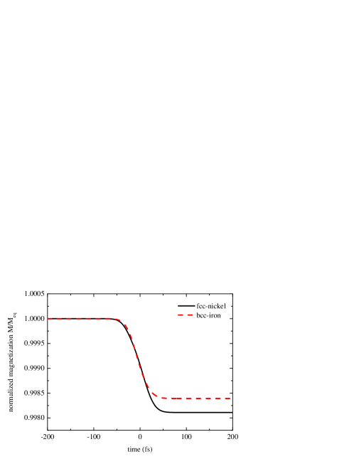
Figure 1: (Color online) Magnetization dynamics due to optical excitation alone. The magnetization is normalized to its equilibrium value.

We first examine the excitation process by the ultrashort optical pulse without including the electron-phonon interaction. We model a homogeneous excitation of a ferromagnetic metal by a laser pulse with gaussian temporal shape, full width at half maximum of 50 fs, and a spectral width of 100 meV at a central photon energy of $\hbar\omega=1.55$ eV. These parameters, as well as the pulse intensity of 4 mJ/cm², are chosen to match typical experimental excitation conditions. To determine the electric field amplitude present in the material we note that the chosen intensity corresponds to an electric field amplitude of $E_{0}=7.5\times 10^{8}$ V/m in vacuum. Reflection at the surface as well as the optical density of the material lead to a reduction of the field amplitude in the material

$$E_{0}^{\prime}=E_{0}\frac{2}{\sqrt{(1+n)^{2}+\kappa^{2}}},$$ (22)

where $n$ and $\kappa$ denote the real and the imaginary part of the refractive index, respectively. Taking $n=2.22$, $\kappa=4.90$ for nickel and $n=2.92$, $\kappa=3.36$ for iron, this leaves us with an amplitude in the material $E_{0}^{\prime}$ of $2.6\times 10^{8}$ V/m for nickel and $2.9\times 10^{8}$ V/m for iron. Johnson and Christy (1974) We take these values of the field amplitude as constant throughout the sample for the calculation and neglect the attenuation due to absorption in the material as well as additional reflection/absorption due to oxide and protection layers. We therefore overestimate the field amplitude present in samples used for the experimental determination of the magnetization dynamics.

The optical excitation contribution alone, i. e., the second term in the dynamical equation (1), leads to the magnetization dynamics shown in Fig. 1. This result should be compared to experimental values for a pulse energy density of 4 mJ/cm², such as those reported in Refs. Krauß et al., 2009 and Carpene et al., 2008 where a “quenching” of the magnetization down to 40 % and 80 % of the equilibrium magnetization was found for nickel and iron, respectively. It is clear from Fig. 1 that the magnetization change computed including only the incoherent optical excitation at the photon energy of 1.55 eV is orders of magnitude smaller than the one observed in experiment.

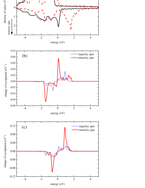
Figure 2: (Color online) Spin-resolved density of states for nickel and iron (a) as well as energy- and spin-resolved occupation change after the optical excitation for nickel (b) and iron (c).

As a contribution to the magnetization change, the optical excitation is negligible, but it is still interesting to take a closer look at the carrier distributions created by the laser pulse because these are essentially the starting point of the momentum-resolved electron-phonon scattering dynamics. To this end, we analyze the energy-dependent occupation changes

$$\Delta N_{\sigma}(\epsilon,t)=\sum_{\vec{k},\mu}\delta(\epsilon-\epsilon_{\vec{k}}^{\mu})\langle\mathcal{P}_{\sigma}\rangle_{\vec{k}}^{\mu}\left[n_{\vec{k}}^{\mu}(t)-f(\epsilon_{\vec{k}}^{\mu},T_{0})\right]$$ (23)

between the dynamical distributions $n_{\vec{k}}^{\mu}(t)$ compared to the equilibrium Fermi-Dirac functions $f(\epsilon_{\vec{k}}^{\mu},T_{0})$ that describe the carrier distributions in equilibrium at the sample temperature $T_{0}$ before the optical excitation. In Eq. (23) we separate occupation changes for minority and majority spins, i. e., for $\sigma=+$ and $-$, respectively, by projecting on the majority and minority spin contributions of the ASW wave functions using the spin-dependent weights (projections)

$$\langle\mathcal{P}_{\sigma}\rangle_{\vec{k}}^{\mu}=\sum_{L}\langle\psi_{\vec{k}}^{\mu}|\mathcal{P}_{\sigma}\psi_{\vec{k}}^{\mu}\rangle_{L}$$ (24)

of each state $\psi_{\vec{k}}^{\mu}$ where

$$\begin{split}\langle\psi_{\vec{k}}^{\mu}|\mathcal{P}_{\sigma}\psi_{\vec{k}}^{\nu}\rangle_{L}&=A_{L\sigma}^{\mu*}(\vec{k})A_{L\sigma}^{\nu}(\vec{k})\langle\tilde{j}|\tilde{j}\rangle_{l\sigma}+C_{L\sigma}^{\mu*}(\vec{k})A_{L\sigma}^{\nu}(\vec{k})\langle\tilde{h}|\tilde{j}\rangle_{l\sigma}\\ &+A_{L\sigma}^{\mu*}(\vec{k})C_{L\sigma}^{\nu}(\vec{k})\langle\tilde{j}|\tilde{h}\rangle_{l\sigma}+C_{L\sigma}^{\mu*}(\vec{k})C_{L\sigma}^{\nu}(\vec{k})\langle\tilde{h}|\tilde{h}\rangle_{l\sigma}\ .\end{split}$$ (25)

The overlaps are given by

$$\langle\tilde{f}|\tilde{g}\rangle_{l\sigma}=\int_{0}^{r_{K}}r^{2}\tilde{f}_{l\sigma}(r)\tilde{g}_{l\sigma}(r)dr.$$ (26)

In this paper, we always use $T_{0}=300$ K as a starting point for the dynamical calculations to facilitate comparison with typical room-temperature measurements. Moreover, room temperature is still less than half the Curie temperature so that we can expect the exchange splitting to be not too different from its $T=0$ K value, and therefore the DFT band structure should be a reasonable approximation.

Figures 2(b) and 2(c) show the spin- and energy-resolved occupation change, computed according to Eq. (23), due to optical excitation at times well after the pump pulse. It corresponds to the magnetization shown in Fig. 1 at $200$ fs. In both materials, mainly minority carriers are excited. The pronounced negative and positive spikes in the minority-spin occupation changes are separated by the photon energy 1.55 eV and roughly coincide with maxima of the density of states [see Fig. 2(a)] for the minority carriers. These maxima stem from the d-bands in these materials, which leads us to conclude that they play a major role in the optical excitation process.

The information about the distribution after the optical excitation contained in Figs. 2(b) and 2(c) allows one to draw conclusions about the maximal magnetization change achievable by electron-phonon scattering in our model, as this distribution is the starting point for the scattering dynamics. Electron-phonon scattering is a quasi-elastic process involving a single-electron, i. e., there is only a small amount of energy transferred in each scattering event. Due to the bath assumption for the phonon system in our calculation, there are also no “secondary electrons” excited because such a transfer of energy to other electrons could only happen mediated by a phonon. We therefore expect that electron-phonon scattering will lead to a continuous relaxation of the excited carriers where the number of non-equilibrium electrons and holes decreases as they are scattered towards the Fermi energy. The demagnetization itself is caused by “spin-flip” scattering processes, i. e., scattering processes with different spin expectation values for initial and final wave functions, that occur during the relaxation process. Therefore the maximal demagnetization that can be caused by scattering in a fixed band structure occurs when all excited majority electrons and minority holes flip their spin while the minority electrons and majority holes do not undergo spin-flip scattering. The relative magnetization change in this physically rather unreasonable case is then given by

$$\max\frac{M}{M_{\text{eq}}}=\frac{\mu_{\text{eq}}-2\left(N_{\text{-}}^{\text{e}}+N_{\text{+}}^{\text{h}}\right)\mu_{B}}{\mu_{\text{eq}}}\ .$$ (27)

Here, $\mu_{B}$ is the Bohr magneton, and $M_{\text{eq}}$ and $\mu_{\text{eq}}$ denote the equilibrium values of the material magnetization and of the magnetic moment per unit cell, respectively. The number of majority electrons $N_{\text{-}}^{\text{e}}$ (minority holes $N_{\text{+}}^{\text{h}}$) per unit cell can be obtained from integrating the occupation changes in Fig. 2 above (below) the Fermi energy. With that estimate we find a minimal relative magnetization due to electron-phonon scattering of 0.84 in nickel and 0.94 in iron, which is a smaller demagnetization than observed in experiments. Without even calculating the full dynamics, we thus expect that microscopic electron-phonon scattering with a fixed band structure is not responsible for the pronounced drop of the magnetization observed in experiments.

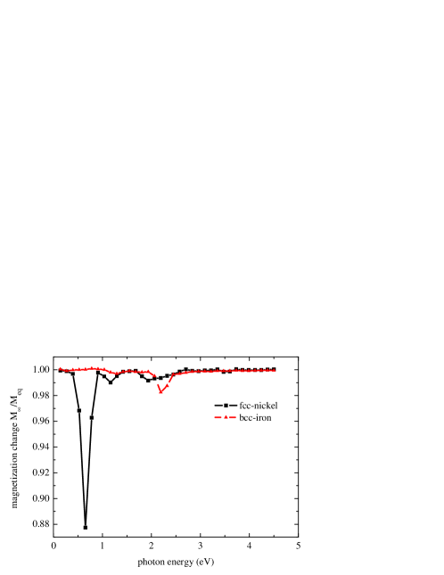
Figure 3: (Color online) magnetization change achievable by optical excitation alone for a range of pump-photon energies.

We next take a closer look at the photon energy dependence of the excitation process. Fig. 3 shows the magnetization change $M_{\infty}/M_{\text{eq}}$ vs. the pump photon energy for a fixed electric field amplitude of $2\times 10^{8}$ V/m. For most of the pump photon energies between 0.1 and 4.5 eV the optical excitation leads to negligible demagnetization, as was discussed above in connection with Fig. 1 for a pump photon energy of 1.55 eV. Only at a pump photon energy of about 0.7 eV for nickel and 2.2 eV for iron one observes a magnetization change of significantly more than 1 %, because these energies correspond to the exchange splitting of the $d$-bands in these materials, so that absorption at these energies is likely to be associated with a change of carrier spin. The order of magnitude of our results for the achievable magnetization change by optical excitation alone seems to be in agreement with those of Zhang et al. Zhang et al. (2009) for the change of magnetization due to the coherent excitation by an optical pulse.

III.2 Electron-phonon scattering

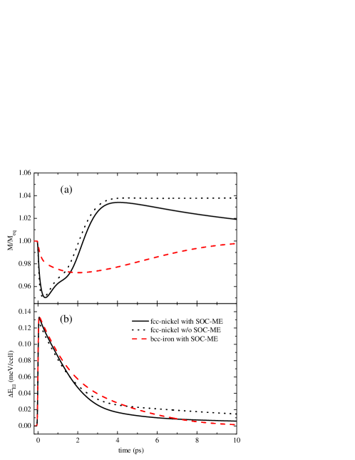
Figure 4: (Color online) Normalized magnetization dynamics (a) and energy difference to equilibrium of the electronic system (b) after the optical excitation including electron-phonon scattering. Results obtained including the spin-orbit coupling contribution in the electron-phonon matrix element are labeled “with SOC-ME.”

In this section, we present results for the carrier dynamics including both optical excitation and electron-phonon scattering. We start by examining in Fig. 4 the magnetization dynamics and the time evolution of the energy in the electronic system for the same parameters that were used in Fig. 1 for the case of optical excitation only. Comparing the magnetization dynamics including electron-phonon scattering in Fig. 4 to those without, cf. in Fig. 1, one notices a demagnetization of about 3–5 %. This magnetization change is smaller than the estimate of the previous section. Due to the scattering, the dynamics now also include a relaxation to equilibrium. This can be made visible by monitoring the energy in the electronic system [Fig. 4(b)], which nicely shows the sudden energy transfer from the laser pulse and a subsequent almost exponential decay with time constants of about 2 ps for nickel and 2.5 ps for iron. These time constants are significantly longer than the electron-phonon coupling times obtained from the analysis of experimental data for these materials ranging from 0.3–0.5 ps. Carpene et al. (2008); Koopmans et al. (2005) Likely, this is because we neglect other scattering mechanisms (such as electron-electron scattering), which open up additional scattering paths and lead to an overall speed-up of the relaxation process. The magnetization for nickel even rises above its value at equilibrium, which is understandable because there is no fundamental law that prohibits non-equilibrium scattering dynamics from going through intermediate states with an increased magnetization. Whether these are reached depends on the band structure, the properties of the states involved, and the initial/excitation conditions.

When comparing the calculated magnetization dynamics to experimental results, one should keep in mind that our calculation neglects changes in the band structure, i.e., the exchange splitting, and the subsequent relaxation of these changes back into equilibrium. Processes associated with the a change of the exchange splitting are expected to dominate the dynamics after a quasi-equilibrium magnetization has been established, namely for times longer than about 5 ps. Djordjevic et al. (2006) A meaningful comparison with experiment of the present model should therefore be limited to a few picoseconds, which is the dynamical time scale for which the different microscopic models mentioned in the introduction have been proposed. In that time window, we find that roughly the same results (which for clarity reasons are only shown for nickel in Fig. 4) are obtained if the spin-orbit term in the interaction matrix elements [cf. Eq. (12)] is neglected.

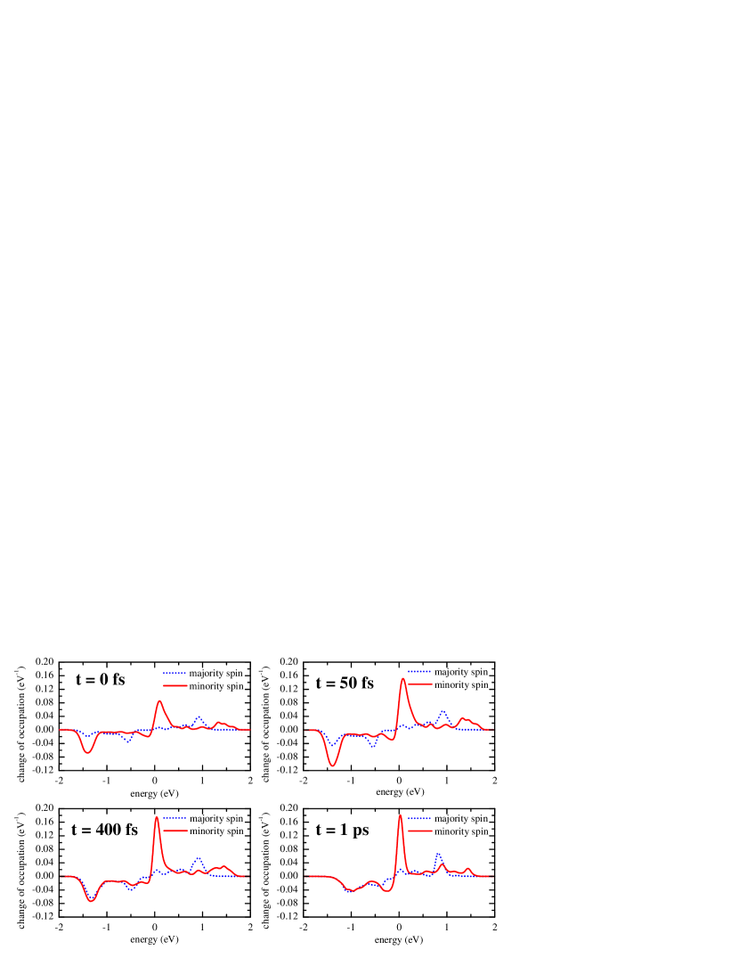
Figure 5: (Color online) Energy- and spin-resolved occupation changes $\Delta N_{\sigma}$ at different times for nickel, as shown in Fig. 4, including the spin-orbit coupling in the electron-phonon matrix element. The representation is in analogy to the one for the optical excitation [Figs. 2(b) and 2(c)].

To get a better understanding of the demagnetization in the present model, it is instructive to look at the carrier distributions at different stages of the dynamics. We present only the results for nickel in this paper, as the carrier dynamics in iron shows similar behavior. In Fig. 5 we plot the energy- and spin-resolved occupation change at different times. Note that after the end of the optical excitation at about 50 fs the excited carrier density above the Fermi energy (at 0 eV) changes only very slowly. In contrast, there is a strong change in the density of holes around 1.4 eV below the Fermi energy. It is the spin-flip of these minority holes that leads to the demagnetization of the material in the present model. The faster dynamics of the holes compared to the excited electrons are due to the difference in the density of states, cf. Fig. 2(a), which is considerably higher below the Fermi energy than above, so that in this energy region there is a larger scattering phase space. In addition, in that energy region there are “spin hot spots,” i. e., points in the Brillouin zone where the states are completely spin-mixed. Their presence also contributes to spin-flip scattering processes. Fabian and Das Sarma (1998)

III.3 Qualitative considerations

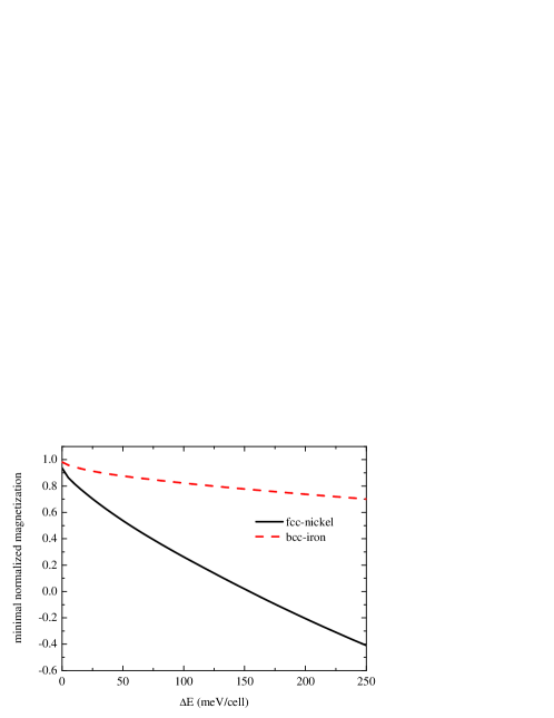
Figure 6: (Color online) Theoretical limit for the minimal magnetization achievable by a pure redistribution in a fixed band structure for a range of deposited energies $\Delta E$.

As we saw from the results of the last section that electron-phonon scattering alone cannot explain the experimentally observed demagnetization, the next important step seems to be to extend the existing model to other scattering mechanisms, e.g., electron-electron or electron-impurity scattering. However, an argument based on energetics shows that their inclusion is not likely to improve the description much, if one retains the limitation that the model contain only scattering, i.e., the redistribution of carriers in a fixed band structure. This conclusion is based on the simple observation that demagnetization in a fixed band structure naturally costs energy as it requires a transfer of occupation from majority states to minority states which are shifted up in energy by the exchange splitting. One can make this observation quantitative by finding the minimal magnetization that the material can attain given a fixed amount of deposited energy $\Delta E$. This leads to a linear optimization problem

$$\min_{\{n_{\vec{k}}^{\mu}:0\leq n_{\vec{k}}^{\mu}\leq 1\}}\sum_{\vec{k}}\!\sum_{\mu}n_{\vec{k}}^{\mu}\left\langle S_{z}\right\rangle_{\vec{k}}^{\mu}$$ (28)

with the following constraints:

$$\sum_{\vec{k}}\!\sum_{\mu}n_{\vec{k}}^{\mu} =N_{\text{eq}}$$ (29a)

$$\sum_{\vec{k}}\!\sum_{\mu}n_{\vec{k}}^{\mu}\epsilon_{\vec{k}}^{\mu} \leq E_{\text{eq}}+\Delta E$$ (29b)

Here $N_{\text{eq}}$ denotes the total number of carriers and $E_{\text{eq}}$ the total energy of the system in equilibrium, i.e., before the arrival of the laser pulse. As before, the contribution from orbital angular momentum to the total magnetization is neglected. We solve this problem with the ab-initio results at hand for a range of deposited energies  $\Delta E$, and show the results in Fig. 6. Note that we present the normalized magnetization, i.e., the minimum obtained from the solution of Eq. (28) divided by the equilibrium magnetization because this value can be readily compared to the demagnetization measured in an experiment. These values represent the minimal magnetization for a carrier distribution in the fixed (equilibrium) band structure given the deposited energy. It holds for all scattering mechanisms that could be creating this distribution provided that they either conserve energy (such as electron-electron scattering) or lead to a loss of energy by transferring it to other systems (such as electron-phonon scattering).

By comparing the experimental demagnetization with the calculated minimal magnetization at the amount of energy deposited in experiment one can see whether the experimental results can, in principle, be explained in terms of scattering alone. This comparison turns out to be not so easy as quite a lot of parameters (e.g. the spot size, absorption, and reflectivity) are necessary for the estimate of the deposited energy from the measured laser intensity and some of them are known only with a considerable uncertainty. That is why we chose to estimate the deposited laser energy directly from the measured magnetization dynamics. This is possible if one relies on two assumptions:

1. At about 5 ps after the laser excitation the scattering processes have locally thermalized the material, so that the initial non-equilibrium dynamics that started has evolved in a quasi-equilibrium dynamics, in which the magnetization at that time can be characterized by the temperature dependence of the magnetization in the ferromagnet $M(t\approx 5\,\text{ps})=M(T)$ where $T=T(t\approx 5\,\text{ps})$.

2. The coupling to the substrate and other losses are so weak that almost all of the energy deposited by the laser is still in the material at that point ($t\approx 5\,\text{ps}$). However, it has been evenly distributed among the inner degrees of freedom.

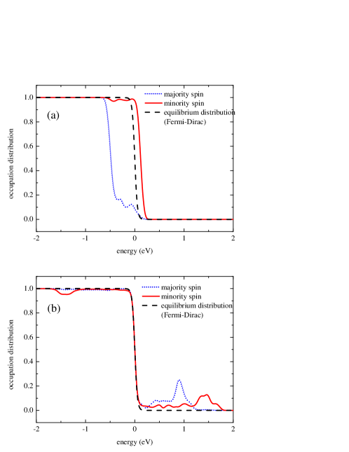
Figure 7: (Color online) Energy- and spin-resolved occupation distributions for nickel. (a) shows the distributions that is necessary to attain the minimal magnetization for $\Delta E=100\,\text{meV}/\text{cell}$ while (b) shows a typical distribution that would be created by the optical excitation (This is a slightly different representation of the data shown in Fig. 2(a). Here we show the occupation distribution which allows an easier comparison with the equilibrium distribution).

These assumptions are consistent with interpretations of measured data by Koopmans et al. Koopmans et al. (2000) and seem to be especially well fulfilled for measurements on thin films. They can now be used to extract the deposited energy from the measured magnetization at 5 ps, and to read off the corresponding achievable minimum magnetization from Fig. 7. This can be compared with the “quenched” magnetization reached in the same measurement. In typical data for nickel and iron at high intensities we find for the normalized magnetization after thermalization values of $M_{\text{Ni}}(5\,\text{ps})=0.1$ and $M_{\text{Fe}}(5\,\text{ps})=0.8$. Using the equilibrium temperature dependence of the magnetization $M(T)$, we conclude that the temperature after local thermalization is about 625 K for nickel and about 800 K for iron, respectively. As we assume an even distribution among the material’s degrees of freedom, we can calculate the deposited energy as an integral over the heat capacity $C_{\text{p}}(T)$:

$$\Delta E=\int_{300\,\text{K}}^{T(5\,\text{ps})}dTC_{\text{p}}(T)$$ (30)

which we solved using experimental data for $C_{\text{p}}(T)$ Landolt-Börnstein (1986) yielding $\Delta E(\text{Ni})=100\,\text{meV}/\text{cell}$ and $\Delta E(\text{Fe})=160\,\text{meV}/\text{cell}$. For these energies, Fig. 6 yields 0.26 and 0.77 as minimal achievable magnetizations for nickel and iron, respectively. These values should be compared to the experimentally observed quenched magnetizations of 0.1 for nickel and 0.7 for iron. As the experimentally measured minima only slightly violate the theoretical bounds, one could be inclined to conclude that this argument does not rule out a demagnetization on the basis of pure redistribution in a fixed band structure. That view changes, however, if one looks at the corresponding distribution functions that are necessary to attain the theoretical magnetization minima. The one for nickel is shown in Fig. 7(a) and should be compared to the distribution that is created by pure optical excitation [Fig. 7(b)]. As discussed before, the optically excited distribution is the starting point for all scattering processes and we would expect these to bring the system back to a Fermi-Dirac distribution (at a higher temperature) which is also displayed in the figure. It is not at all likely that in the course of this process there will be an intermediate state that has a distribution that is anywhere close to the one shown in Fig. 7(a) for two reasons: First, for a magnetization close to the theoretical limit a highly “ordered” distribution is necessary, which is unlikely to be reached by random scattering processes. Second, the state shown in Fig. 7(a) lies very far off from the direct continuous transition from the distribution in Fig. 7(b) to the equilibrium distribution, both in terms of a simple relaxation time approximation and if one considers a quasi-elastic process, such as electron-phonon scattering, where we have a slow, but continuous energy relaxation of the exited carriers towards the Fermi energy where eventually non-equilibrium electrons and holes cancel out.

Even though this argument is not a rigorous, we find it convincing enough to draw the conclusion that scattering dynamics in a fixed band structure cannot explain the observed ultrafast demagnetization. It is therefore important to include the dynamical changes in the band structure, i.e., the exchange splitting, in a comprehensive microscopic theory of ultrafast demagnetization in ferromagnets.

IV Conclusions

The main objective of this paper was to analyze in detail the dynamics due to one of the proposed mechanisms for ultrafast demagnetization: the Elliott-Yafet process based on electron-phonon scattering. To this end, we carried out a numerical analysis without adjustable parameters including the laser excitation and the scattering dynamics on the level of Boltzmann scattering integrals. We evaluated the model for the elementary ferromagnets nickel and iron utilizing realistic band structures and matrix elements obtained from ab-initio calculations. As in previous studies, Krauß et al. (2009); Steiauf and Fähnle (2009) we kept the band structure fixed. In this case, the computed demagnetization for realistic pump-laser intensities is smaller by almost a factor of ten than what is observed in experiments. An additional argument shows that this bound for the achievable magnetization “quenching” is likely to hold as well for other scattering mechanisms, such as electron-electron or electron-impurity scattering. We interpret our numerical results that any fully microscopic model that tries to explain ultrafast demagnetization by scattering dynamics really should include a dynamical change of the band structure, i.e., the exchange splitting. A microscopic determination of this change seems more important for the understanding of the demagnetization process than studies focussing on Elliott-Yafet-type mechanisms.

Appendix A Numerical Method

For the numerical solution of Eq. (1) we replace the energy delta function in the scattering rates, Eq. (4), by a gaussian of finite width to allow a Brillouin zone integration on the chosen grid of $\vec{k}$-points. The FWHM of this broadened distribution is taken to be 15 meV for the DFT grid at hand, and convergence of the results with respect to grid size and distribution width was checked.

A.1 Reducing the dimensionality of the problem

Two simplifications help to reduce the numerical effort for the solution of Eq. (1):

The first is based on the fact that only the states in a limited energy range around the Fermi energy will experience an occupation change in the course of the dynamics. Due to the structure of the equilibrium distribution

$$(n_{\vec{k}}^{\mu})_{\text{eq}}=\frac{1}{e^{\left(\epsilon_{\vec{k}}^{\mu}-\mu\right)/k_{B}T_{0}}+1}$$ (31)

the states far ($\geq 200\,\text{meV}$ for $T_{0}=300\,\text{K}$) above the Fermi energy ($\mu\approx E_{F}$) will be empty while those far below the Fermi energy will be fully occupied. As the incoming laser pulse will only cause resonant transitions between occupied and unoccupied states, the occupation change due to the optical excitation is limited to an energy range around the Fermi energy. This is clearly seen in the energy resolved occupation change due to the optical excitation in Fig. 2. States far away from the Fermi energy ($\bigl{|}\epsilon_{\vec{k}}^{\mu}-E_{F}\bigr{|}\gg E_{\text{las}}$) remain at their equilibrium values. As the electron-phonon scattering transfers only small amounts of energy in each scattering process, the occupation of these states is not influenced by the following scattering dynamics either. That is why one can safely assume the occupation of these states to remain constant in time. Only states in an energy range $\bigl{|}\epsilon_{\vec{k}}^{\mu}-E_{F}\bigr{|}\leq\delta E$ are actually included in the dynamical calculation of the occupation numbers. So, for each $\vec{k}$-point, we only include the subset of bands $n_{\vec{k}}^{\mu_{j}}$ into the dynamical calculation that fall in the chosen energy range $\delta E$. For the calculations including only the optical excitation in Sec. III.1 we took $\delta E$ to be 5 eV, but for the photon energy under investigation (1.55 eV) a much smaller range actually suffices. We therefore reduced it to 2 eV for the calculations including scattering in Sec. III.2.

The second simplification can be made due to the crystal symmetries of the materials under investigation. These symmetries imply that the wave functions of two states at different $\vec{k}$-points which are related by a crystal symmetry operation are also connected by the same symmetry operation. From that one can deduce that the modulus of an electron-phonon matrix element between two states does not change if one applies a crystal symmetry operation on the initial and the final state. In other words, electron-phonon scattering will not break the symmetry of an occupation distribution that has the same symmetry as the crystal (e.g., the thermal distribution before optical excitation). The optical excitation could break that symmetry as it involves the scalar product with an external electric field. In our paper, we restrict ourselves to the description of the typical experimental case where the laser field is parallel to the material magnetization so that the symmetry of the occupation distribution is not broken by the optical excitation. In this case, it is not necessary to compute all occupation numbers $n_{\vec{k}}^{\mu}$. Rather all information about the occupation distribution is contained in any subset $\{\vec{k}_{j}\}$ of $\vec{k}$-points which constitutes an irreducible wedge of the Brillouin zone.

A.2 Numerical evaluation

With these two simplifications we are left with a subset of occupation numbers $n_{j}$ which need to be calculated dynamically. Here $j=(\vec{k}_{j},\mu_{j})$ denotes a multi-index that includes the $\vec{k}$-point as well as the band index of the state. With the help of this notation, Eq. (1) can be reformulated to yield

$$\frac{\partial n_{j}}{\partial t}=\left.\frac{\partial n_{j}}{\partial t}\right|_{\text{opt}}+\left.\frac{\partial n_{j}}{\partial t}\right|_{\text{e-p}}=\left|\vec{E}(t)\right|^{2}\sum_{i}\mathbf{B}_{ji}^{\text{opt}}n_{i}+\sum_{i}\left(n_{j}\mathbf{A}_{ji}^{\text{e-p}}\left(1-n_{i}\right)-\left(1-n_{j}\right)\mathbf{A}_{ij}^{\text{e-p}}n_{i}\right),$$ (32)

where all $n_{j}$-independent quantities are contained in the constant matrices $\mathbf{A}^{\text{e-p}}$ and $\mathbf{B}^{\text{opt}}$, which can be precomputed for the chosen set of states. Interpreting the occupation numbers $n_{j}$ as a vector $\vec{n}$ we can alternatively write this as

$$\frac{\partial}{\partial t}\vec{n}=\left|\vec{E}(t)\right|^{2}\mathbf{B}^{\text{opt}}\vec{n}+\text{diag}\left(\vec{n}\right)\mathbf{A}^{\text{e-p}}\left(\vec{1}-\vec{n}\right)-\text{diag}\left(\vec{1}-\vec{n}\right)\left(\mathbf{A}^{\text{e-p}}\right)^{T}\vec{n}$$ (33)

where $\text{diag}(\vec{n})$ is a matrix with the occupation numbers on the diagonal. $\vec{1}$ denotes a vector with all entries set to one. In the form of Eq. (33) the differential equation is especially well suited for a numerical evaluation. We used a MATLAB algorithm Shampine and Reichelt (1997) for the solution.

References

- Beaurepaire et al. (1996) E. Beaurepaire, J.-C. Merle, A. Daunois, and J.-Y. Bigot, Phys. Rev. Lett. 76, 4250 (1996).
- Koopmans et al. (2010) B. Koopmans, G. Malinowski, F. Dalla Longa, D. Steiauf, M. Fähnle, T. Roth, M. Cinchetti, and M. Aeschlimann, Nat. Mater. 9, 259 (2010).
- Stamm et al. (2007) C. Stamm, T. Kachel, N. Pontius, R. Mitzner, T. Quast, K. Holldack, S. Khan, C. Lupulescu, E. F. Aziz, M. Wietstruk, H. A. Dürr, and W. Eberhardt, Nat. Mater. 6, 740 (2007).
- Carva et al. (2009) K. Carva, D. Legut, and P. M. Oppeneer, Europhys. Lett. 86, 57002 (2009).
- Carpene et al. (2008) E. Carpene, E. Mancini, C. Dallera, M. Brenna, E. Puppin, and S. De Silvestri, Phys. Rev. B 78, 174422 (2008).
- Zhang and Hübner (2000) G. P. Zhang and W. Hübner, Phys. Rev. Lett. 85, 3025 (2000).
- Zhang et al. (2009) G. P. Zhang, Y. Bai, and T. F. George, Phys. Rev. B 80, 214415 (2009).
- Lefkidis and Hübner (2009) G. Lefkidis and W. Hübner, J. Magn. Magn. Mater. 321, 979 (2009).
- Atxitia et al. (2010) U. Atxitia, O. Chubykalo-Fesenko, J. Walowski, A. Mann, and M. Münzenberg, Phys. Rev. B 81, 174401 (2010).
- Krauß et al. (2009) M. Krauß, T. Roth, S. Alebrand, D. Steil, M. Cinchetti, M. Aeschlimann, and H. C. Schneider, Phys. Rev. B 80, 180407 (2009).
- Koopmans et al. (2005) B. Koopmans, J. J. M. Ruigrok, F. Dalla Longa, and W. J. M. de Jonge, Phys. Rev. Lett. 95, 267207 (2005).
- Walowski et al. (2008) J. Walowski, G. Müller, M. Djordjevic, M. Münzenberg, M. Kläui, C. A. F. Vaz, and J. A. C. Bland, Phys. Rev. Lett. 101, 237401 (2008).
- Steiauf and Fähnle (2009) D. Steiauf and M. Fähnle, Phys. Rev. B 79, 140401 (2009).
- Steiauf et al. (2010) D. Steiauf, C. Illg, and M. Fähnle, J. Magn. Magn. Mater. 322, L5 (2010).
- Battiato et al. (2010) M. Battiato, K. Carva, and P. M. Oppeneer, Phys. Rev. Lett. 105, 027203 (2010).
- Williams et al. (1979) A. R. Williams, J. Kübler, and C. D. Gelatt Jr., Phys. Rev. B 19, 6094 (1979).
- Kübler (2000) J. Kübler, Theory of Itinerant Electron Magnetism (Oxford University Press, New York, 2000).
- Eyert (2007) V. Eyert, The Augmented Spherical Wave Method, Lecture Notes in Physics, Vol. 719 (Springer Berlin Heidelberg, Berlin, Heidelberg, 2007).
- Grimvall (1981) G. Grimvall, The Electron-Phonon Interaction in Metals (North-Holland, 1981).
- Yafet (1963) Y. Yafet, in Solid State Physics, Vol. 14, edited by F. Seitz and D. Turnbull (New York, 1963).
- Oppeneer et al. (1992) P. M. Oppeneer, T. Maurer, J. Sticht, and J. Kübler, Phys. Rev. B 45, 10924 (1992).
- Gray (1972) D. E. Gray, ed., American Institute of Physics Handbook, 3rd ed. (McGraw-Hill, 1972).
- Giannozzi et al. (2009) P. Giannozzi, S. Baroni, N. Bonini, M. Calandra, R. Car, C. Cavazzoni, D. Ceresoli, G. L. Chiarotti, M. Cococcioni, I. Dabo, A. Dal Corso, S. de Gironcoli, S. Fabris, G. Fratesi, R. Gebauer, U. Gerstmann, C. Gougoussis, A. Kokalj, M. Lazzeri, L. Martin-Samos, N. Marzari, F. Mauri, R. Mazzarello, S. Paolini, A. Pasquarello, L. Paulatto, C. Sbraccia, S. Scandolo, G. Sclauzero, A. P. Seitsonen, A. Smogunov, P. Umari, and R. M. Wentzcovitch, J. Phys.: Condens. Matter 21, 395502 (2009).
- Dal Corso and de Gironcoli (2000) A. Dal Corso and S. de Gironcoli, Phys. Rev. B 62, 273 (2000).
- Johnson and Christy (1974) P. B. Johnson and R. Christy, Phys. Rev. B 9, 5056 (1974).
- Djordjevic et al. (2006) M. Djordjevic, M. Lüttich, P. Moschkau, P. Guderian, T. Kampfrath, R. G. Ulbrich, M. Münzenberg, W. Felsch, and J. S. Moodera, Phys. Status Solidi C 3, 1347 (2006).
- Fabian and Das Sarma (1998) J. Fabian and S. Das Sarma, Phys. Rev. Lett. 81, 5624 (1998).
- Koopmans et al. (2000) B. Koopmans, M. van Kampen, J. T. Kohlhepp, and W. J. M. de Jonge, Phys. Rev. Lett. 85, 844 (2000).
- Note (1) Measurements Koopmans et al. (2010) on Ni (15\tmspace+.1667emnm) film with 5.0\tmspace+.1667emmJ/cm2.
- Note (2) Measurements Carpene et al. (2008) on Fe (7\tmspace+.1667emnm) film with 6.0\tmspace+.1667emmJ/cm2.
- Landolt-Börnstein (1986) Landolt-Börnstein, Magnetic Properties of Metals: III/19A, edited by H. P. J. Wijn (Springer Berlin Heidelberg, 1986).
- Shampine and Reichelt (1997) L. F. Shampine and M. W. Reichelt, SIAM J. Sci. Comput. 18, 1 (1997).