Stepping Lazy Programs

Abstract

Debugging lazy functional programs poses serious challenges. In support of the “stop, examine, and resume” debugging style of imperative languages, some debugging tools abandon lazy evaluation. Other debuggers preserve laziness but present it in a way that may confuse programmers because the focus of evaluation jumps around in a seemingly random manner.

In this paper, we introduce a supplemental tool, the algebraic program stepper. An algebraic stepper shows computation as a mathematical calculation. Algebraic stepping could be particularly useful for novice programmers or programmers new to lazy programming. Mathematically speaking, an algebraic stepper renders computation as the standard rewriting sequence of a lazy $\lambda$-calculus. Our novel lazy semantics introduces lazy evaluation as a form of parallel program rewriting. It represents a compromise between Launchbury’s store-based semantics and a simple, axiomatic description of lazy computation as sharing-via-parameters, à la Ariola et al. Finally, we prove that the stepper’s run-time machinery correctly reconstructs the standard rewriting sequence.

azy programming; debugging and stepping; lazy lambda calculus

1 How Functional Programming Works

Hughes1989WhyFPMatters explains why functional programming matters. By “functional programming” Hughes specifically means “lazy” functional programming, and by “matters” he refers to the distinct advantages of laziness for programming with reusable components, i.e., functions and programs. Hughes’s examples demonstrate the ease of creating functions and programs by gluing together existing functions and programs. The key advantage of laziness is that even if one component appears to produce too much data, the laziness of the consuming component almost always naturally eliminates the superfluous data production. Since then, numerous researchers have extended this argument with examples of their own, usually accompanied by elegant code in Haskell.

Unfortunately, laziness also increases the distance between the programmer and the underlying machinery. Specifically, laziness reduces a programmer’s ability to predict when certain expressions are evaluated during program execution. As long as things work, this cognitive dissonance poses no problems. When a program exhibits erroneous behavior, however, programmers are often at a loss. A programmer can turn to a debugger for help, but the evaluation of lazy programs is often confusing enough that lazy debuggers resort to hiding laziness from the programmer in order to display useful information Wallace et al. (2001); Ennals and Peyton Jones (2003a); Allwood et al. (2009).

An ideal debugger should not modify the execution model of a program. The maintainers of the Glasgow Haskell Compiler Peyton Jones et al. (1992) share this sentiment, since the bundled GHCi debugger abides by this ideal. The authors of the GHCi debugger Marlow et al. (2007) state that their debugger “lets the programmer see the effects of laziness,” and therefore, “shows the programmer what is actually happening in their program at runtime”. Unfortunately, the authors also acknowledge that their debugger presents lazy computations in a way that is difficult to follow, mostly through seemingly random jumps from one place to another in the program.

To mitigate the drawbacks of existing lazy debuggers, we propose a supplementary tool, the algebraic stepper. PLT’s DrRacket Findler et al. (2002) comes with such a stepper for the call-by-value Racket language. Given a functional program, the algebraic stepper displays its standard reduction sequence in the by-value $\lambda$-calculus Clements et al. (2001). Our experience suggests that this kind of tool especially benefits novice programmers when they try to understand small programs, and programmers who are new to the language and are trying to explore some linguistic feature.

DrRacket’s stepper presents evaluation of a program directly as a manipulation of the source, similar to the calculated manipulations of a student of mathematics. We conjecture that this model is suitable for addressing the confusing nature of lazy evaluation. In this paper, we present: (1) our stepper for Lazy Racket Barzilay and Clements (2005); (2) its underlying semantics, a novel lazy $\lambda$-calculus; (3) and a proof that the stepper correctly implements the standard rewriting semantics of the calculus. Roughly speaking, Lazy Racket is a call-by-need language that uses the same evaluation mechanism as Haskell. A Lazy Racket module macro-expands its surface syntax into a plain Racket program enriched with appropriate delay and force constructs Hatcliff and Danvy (1997). Lazy Racket is mostly used in educational settings—where we have tested the prototype of the stepper so far—though some programmers have found it useful to construct parser combinators or game trees in Lazy Racket modules, and then to export such pieces to plain Racket modules.

The novel lazy $\lambda$-calculus introduces the idea of selective parallel reduction to simulate shared reductions. On the one hand, it is nearly trivial to prove an equivalence between the standard rewriting semantics of our calculus and a Launchbury-style, store-based semantics Launchbury (1993). On the other hand, the calculus is the appropriate basis for a correctness proof of the stepper. For the correctness proof, we construct a model of the delay-and-force implementation, further enriched with continuation marks Clements et al. (2001), show that it bisimulates the standard rewriting semantics, and finally, exploit Clements’s strategy for the rest of the proof Clements (2006).

Section 2 briefly introduces Lazy Racket and its stepper. Section 3 presents a novel lazy $\lambda$-calculus and its essential theorems. Section 4 summarizes the essential details of the implementation of Lazy Racket and presents a model of the lazy stepper. Section 5 presents a correctness proof for the stepper and the penultimate section summarizes related work.

2 Lazy Racket and Its Stepper

Lazy Racket programs are sequences of defines and expressions that usually refer to the definitions. Here is a basic example:

        (define (f x) (+ x x))
        (f (+ 1 (+ 2 3)))

A programmer invokes the Lazy Racket stepper from the DrRacket IDE. Running the stepper displays the reduction sequence for the current program. Figure 1 shows a sequence of screenshots stepping through the above program, with each shot displaying one reduction step.

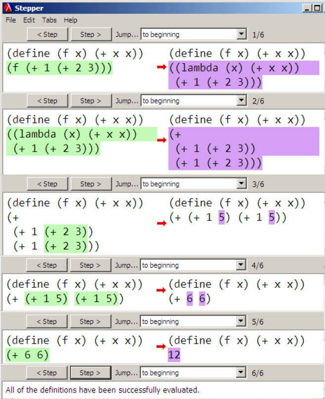
Figure 1: Lazy Stepper Example 1

A green box highlights the redex(es) on the left-hand side of a reduction step and a purple box highlights the contractum(s) on the right-hand side. The programmer can navigate the reduction sequence in either the forward or backward direction. Additional navigation features are in the planning stages.

In step 2, evaluation of the function argument is delayed so an unevaluated argument replaces each instance of the variable x in the function body. In step 3, evaluation of the program at the first x position requires the value of the argument, so the argument is forced in steps 3 and 4. In steps 3 and 4, all shared instances of the argument are reduced simultaneously. That is, the stepper explains evaluation as an algebraic process using a form of parallel reduction. Since the second x refers to the same delayed computation as the first x, by the time evaluation of the program requires a value at the second x position, a result is already available because the computed value of the first x was saved. In short, no argument evaluation is repeated.

A second example introduces the lazy take! function, which extracts the first n elements of a specified list:

  (define (take! n lst)
    (if (= n 0)
        null
        (cons (first lst)
              (take! (- n 1) (rest lst)))))
  (define (f lst) (+ (first lst) (second lst)))
  (f (take! 3 (list 1 2 (/ 1 0) 4)))

The reduction sequence for this program, as viewed in the stepper, appears in figure 2. For space reasons, only interesting steps are shown.

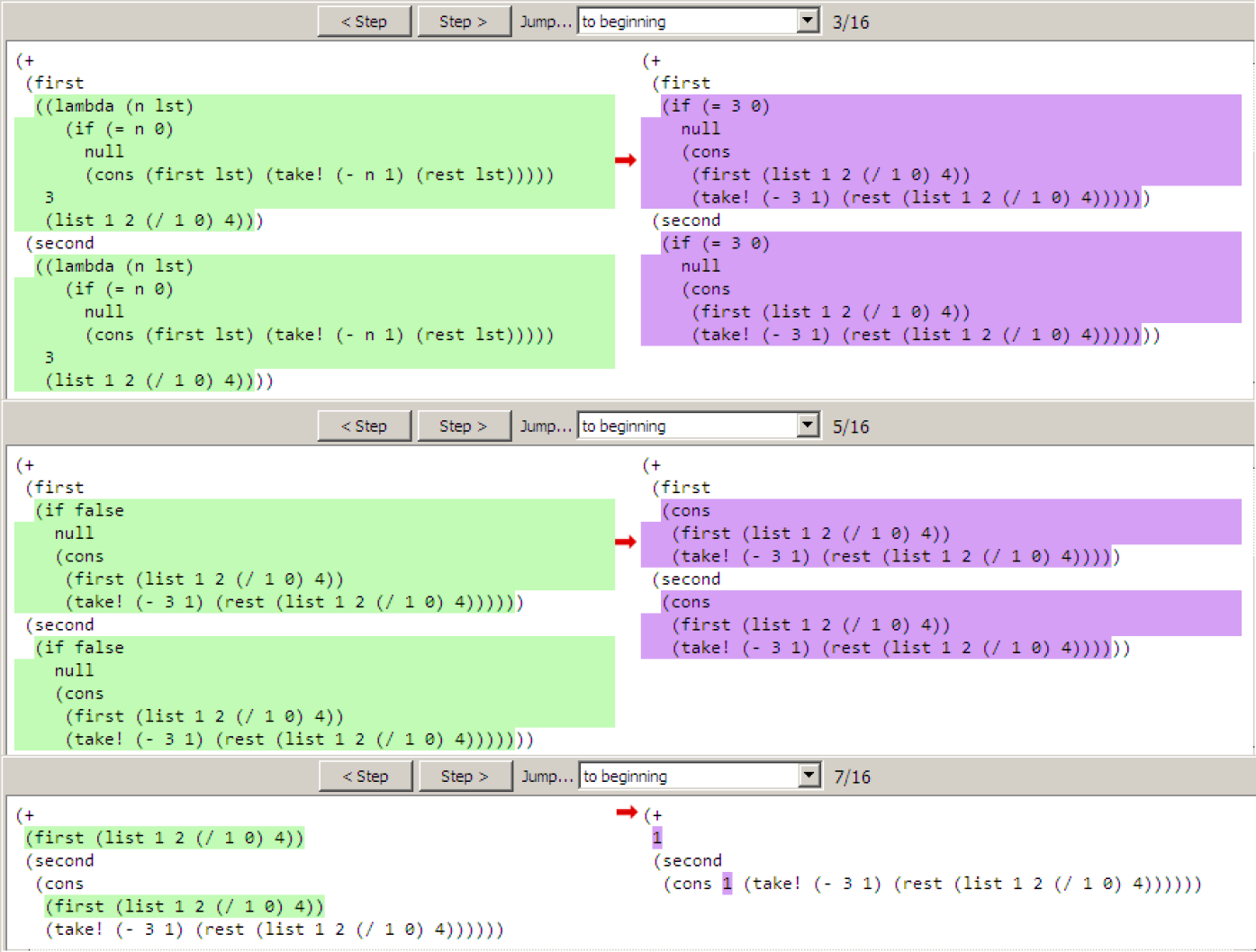
Figure 2: Lazy Stepper Example 2

In this example, the result of the take! computation is the argument to the function f. The take! computation extracts the first three elements of its list argument, but f only uses the first two list elements, so the third element, which produces an error, should not be forced. In step 3, the take! computation is forced because both + and first are strict. In Lazy Racket, cons behaves lazily and does not evaluate its arguments Friedman and Wise (1976), so in step 5, the result of the take! computation is a cons with two thunks: one that retrieves the first element of the list, and one that contains the next iteration of the take! computation. In step 7, the first addition operand is finally reduced to a value. Notice that the first element in the argument to second is already reduced as well. The remaining steps force the next iteration of take! and similarly extract the second element of the list. Since only the first two elements of the list are needed, no additional take! iterations are computed and the division by zero never raises an error.

A third example involves infinite lists:

    (define (add-one x) (+ x 1))
    (define nats (cons 1 (map add-one nats)))
    (+ (second nats) (third nats))

More importantly, it involves map, which the stepper has not annotated because it is a library function. The reduction sequence for this program appears in figure 3. Again, some function definitions and reduction steps have been elided from the screenshots.

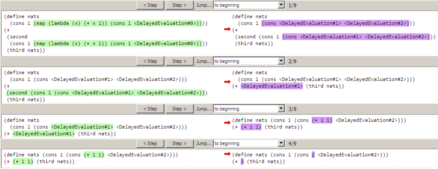
Figure 3: Lazy Stepper Example 3

In step 1, the evaluation of second forces the map expression to a cons containing two thunks. Unlike the second example, the thunks are displayed as <DelayedEvaluation#1> and <DelayedEvaluation#2> because their contents are unknown, i.e., they were not part of the source program. In step 2, the second expression extracts <DelayedEvaluation#1> from the list, but the thunk is still unevaluated. In steps 3 and 4, evaluation of the program requires the value of <DelayedEvaluation#1>, so it is forced. Observe how the stepper updates the nats definition with the result as well. The remaining steps show the similar evaluation of the other addition operand and are thus omitted.

As a final example, we use our stepper to understand the behavior of a program presented by Marlow2007Debugger:

;; [Listof Char] -> [Listof [Listof Char]]
(define (lines s)
 (cond
   [(null? s) null]
   [else
    (define-values (l t)
      (break (lambda (x) (equal? "\n" x)) s))
    (cons l (cond
              [(null? t) null]
              ; drop "\n" char and recur
              [else (lines (cdr t))]))]))

;; [Char -> Boolean] [Listof Char]
;;  ->* [Listof Char] [Listof Char]
(define (break p? l)
  (let L ([l l] [line null])
    (cond
      [(null? l) (values (reverse line) null)]
      [(p? (car l)) (values (reverse line) l)]
      [else (L (cdr l) (cons (car l) line))])))

The break function consumes two arguments, a predicate on characters and a string represented as a list of characters, and splits the string at the first character for which the predicate is true, returning two substrings simultaneously. The delimiting character remains as the first character of the second substring. The lines function uses break to separate an input string into lines, where a "\n" character begins a new line. Unlike break, the delimiting character is not included in the output of lines.

Evaluating the expression (lines ’("\n" "a")) produces the expected result, an empty line (the empty string) and a line with one "a" character (the !! function is a recursive force function):

    > (!! (lines ’("\n" "a")))
    ’(() ("a"))

However, (lines ’("a" "\n")) produces only one line:

    > (!! (lines ’("a" "\n")))
    ’(("a"))

Marlow2007Debugger show how to use the GHCi debugger to understand this behavior. Figure 4 demonstrates that the stepper provides a superior vehicle in this situation. It specifically shows how break returns two values, which when evaluated, produce a one-character string "a" and a one-character string "\n", respectively. From the remainder of the definition of lines, we can deduce that the "a" string is retained, while the "\n" is dropped by the subsequent call to cdr, causing the recursive lines call to return an empty list, i.e. no lines, thus explaining the missing line. If we want lines to output a final, empty line when there is a trailing "\n" in the input, the base case must return a list with an empty line, ’(()), instead of just an empty list.

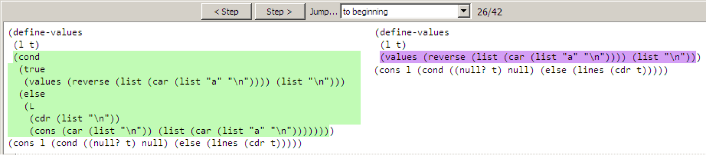
Figure 4: Lazy Stepper Example 4

3 Lazy Racket Semantics

Our key theoretical innovation is the novel semantic view of laziness displayed in our stepper. Following tradition, we present this idea in the context of a $\lambda$-calculus, $\lambda_{\textsc{lr}}$:

$$e= \;n\mid s\mid b\mid x\mid\lambda x.e\mid(e\;e)\mid(p^{2}\;e\;e)$$

$$\mid(\texttt{cons}\;e\;e)\mid\texttt{null}\mid(p^{1}\;e)\mid(\texttt{if}\;e\;e\;e)$$

$$n\in \;\mathbb{Z},\;s\in\textrm{Strings},\;b=\texttt{true}\mid\texttt{false}$$

$$p^{2}= \;+\mid-\mid*\mid/\hskip 14.22636ptp^{1}=\texttt{first}\mid\texttt{rest}$$

The syntax of $\lambda_{\textsc{lr}}$ is identical to the core of most functional programming languages and includes integers, strings, booleans, variables, abstractions, applications, primitives, lists, and a conditional.

To specify the semantics of $\lambda_{\textsc{lr}}$, we first extend $e$ by adding a new expression:

$$e^{\textsc{lr}} =e\mid{e^{\textsc{lr}}}^{\ell}\hskip 14.22636pt\ell\in\textrm{Labels}$$

The “labeled” expression, ${e^{\textsc{lr}}}^{\ell}$, consists of a tag $\ell$ and a subexpression $e^{\textsc{lr}}$. Labeled expressions are not part of the language syntax but are necessary for evaluation. Rewriting a labeled expression triggers the simultaneous rewriting of all other expressions that share the same label. Otherwise, labeled expressions do not affect program evaluation. The stepper renders labeled expressions without the label.

We require one constraint on labeled expressions in our language: all expressions with the same label $\ell$ must be identical. We call this the consistent labeling property:

Definition 1.

A program is consistently labeled if, for all $\ell_{1}$, $\ell_{2}$, $e^{\textsc{lr}}_{1}$, $e^{\textsc{lr}}_{2}$, if ${e^{\textsc{lr}}_{1}}^{\ell_{1}}$ and ${e^{\textsc{lr}}_{2}}^{\ell_{2}}$ are two subexpressions in a program, and $\ell_{1}=\ell_{2}$, then $e^{\textsc{lr}}_{1}=e^{\textsc{lr}}_{2}$.

LHS               $\longmapsto_{\textsc{lr}}$                       RHS
	$\nexists E_{1},E_{2},\ell$	$E[\>]=E_{1}[{(E_{2}[\>])}^{\ell}]$
	s.t. $E[\>]=E_{1}[{(E_{2}[\>])}^{\ell}]$	$\nexists E_{3},E_{4},\ell^{\prime}$ s.t. $E_{2}[\>]=E_{3}[{(E_{4}[\>])}^{\ell^{\prime}}]$
	(redex not under label)	(redex occurs under label)
$E[({(\lambda x.e^{\textsc{lr}}_{1})}^{\vec{\ell}}\;e^{\textsc{lr}}_{2})]$	$E[e^{\textsc{lr}}_{1}\{x:={e^{\textsc{lr}}_{2}}^{\ell_{1}}\}]$	$E[e^{\textsc{lr}}_{1}\{x:={e^{\textsc{lr}}_{2}}^{\ell_{1}}\}]\{\!\!\{\ell\Leftarrow E_{2}[e^{\textsc{lr}}_{1}\{x:={e^{\textsc{lr}}_{2}}^{\ell_{1}}\}]\}\!\!\}$	$\beta_{LR}$
	$\texttt{fresh}\;\ell_{1}$	$\texttt{fresh}\;\ell_{1}$
$E[(p^{2}\;{n_{1}}^{\vec{\ell}}\;{n_{2}}^{\vec{\ell}})]$	$E[(\delta\;(p^{2}\;n_{1}\;n_{2}))]$	$E[(\delta\;(p^{2}\;n_{1}\;n_{2}))]\{\!\!\{\ell\Leftarrow E_{2}[(\delta\;(p^{2}\;n_{1}\;n_{2}))]\}\!\!\}$	Prim
$E[(\texttt{cons}\;e^{\textsc{lr}}_{1}\;e^{\textsc{lr}}_{2})]$	$E[(\texttt{cons}\;{e^{\textsc{lr}}_{1}}^{\ell_{1}}\;{e^{\textsc{lr}}_{2}}^{\ell_{2}})]$	$E[(\texttt{cons}\;{e^{\textsc{lr}}_{1}}^{\ell_{1}}\;{e^{\textsc{lr}}_{2}}^{\ell_{2}})]\{\!\!\{\ell\Leftarrow E_{2}[(\texttt{cons}\;{e^{\textsc{lr}}_{1}}^{\ell_{1}}\;{e^{\textsc{lr}}_{2}}^{\ell_{2}})]\}\!\!\}$	Cons
$e^{\textsc{lr}}_{1}\textrm{ unlabeled or }e^{\textsc{lr}}_{2}\textrm{ unlabeled}$	$\texttt{fresh}\;\ell_{1},\ell_{2}$	$\texttt{fresh}\;\ell_{1},\ell_{2}$
$E[(\texttt{first}\;{(\texttt{cons}\;e^{\textsc{lr}}_{1}\;e^{\textsc{lr}}_{2})}^{\vec{\ell}})]$	$E[e^{\textsc{lr}}_{1}]$	$E[e^{\textsc{lr}}_{1}]\{\!\!\{\ell\Leftarrow E_{2}[e^{\textsc{lr}}_{1}]\}\!\!\}$	First
$E[(\texttt{rest}\;{(\texttt{cons}\;e^{\textsc{lr}}_{1}\;e^{\textsc{lr}}_{2})}^{\vec{\ell}})]$	$E[e^{\textsc{lr}}_{2}]$	$E[e^{\textsc{lr}}_{2}]\{\!\!\{\ell\Leftarrow E_{2}[e^{\textsc{lr}}_{2}]\}\!\!\}$	Rest
$E[(\texttt{if}\;{\texttt{true}}^{\vec{\ell}}\;e^{\textsc{lr}}_{1}\;e^{\textsc{lr}}_{2})]$	$E[e^{\textsc{lr}}_{1}]$	$E[e^{\textsc{lr}}_{1}]\{\!\!\{\ell\Leftarrow E_{2}[e^{\textsc{lr}}_{1}]\}\!\!\}$	If-true
$E[(\texttt{if}\;{\texttt{false}}^{\vec{\ell}}\;e^{\textsc{lr}}_{1}\;e^{\textsc{lr}}_{2})]$	$E[e^{\textsc{lr}}_{2}]$	$E[e^{\textsc{lr}}_{2}]\{\!\!\{\ell\Leftarrow E_{2}[e^{\textsc{lr}}_{2}]\}\!\!\}$	If-false

Figure 5: The $\lambda_{\textsc{lr}}$ Reduction System.

3.1 Rewriting Rules

To further formulate a semantics, we define the notion of values:

$$v=n\mid s\mid b\mid\lambda x.e^{\textsc{lr}}\mid\texttt{null}\mid(\texttt{cons}\;{e^{\textsc{lr}}}^{\ell}\;{e^{\textsc{lr}}}^{\ell})\mid{v}^{\ell}$$

Numbers, strings, booleans, abstractions, and null are values. In addition, cons expressions where each element is labeled are also values. Finally, any value tagged with labels is also a value.

In the rewriting of $\lambda_{\textsc{lr}}$ programs, evaluation contexts are used to determine which part of the program to rewrite next. Evaluation contexts are expressions where a hole $[\;]$ replaces one subexpression:

$$E=[\;] \mid(E\;e^{\textsc{lr}})\mid(p^{2}\;E\;e^{\textsc{lr}})\mid(p^{2}\;v\;E)\mid(p^{1}\;E)$$

$$\mid(\texttt{if}\;E\;e^{\textsc{lr}}\;e^{\textsc{lr}})\mid{E}^{\ell}$$

The $(E\;e^{\textsc{lr}})$ context indicates that the operator in an application is evaluated before it is applied. The $p^{1}$ and $p^{2}$ contexts indicate that these primitives are strict in all argument positions. The if context dictates strict evaluation of only the test expression. Finally, the ${E}^{\ell}$ context dictates that a redex search goes under labeled expressions. Essentially, when searching for a redex, expressions tagged with a label are treated as if they were unlabeled.

Evaluation of a $\lambda_{\textsc{lr}}$ program proceeds according to the program rewriting system in figure 5. For each possible rewriting step, the program in the first column is partitioned into a redex and a context, and is rewritten to either the program in the second or the third column. In the second and third columns, the redex is always contracted. If the redex does not occur under a label, then it is the only contracted part of the program (column two). If the redex occurs under a label, all other instances of the label are similarly contracted (column three). In the third column, the context is further subdivided as $E[\>]=E_{1}[{(E_{2}[\>])}^{\ell}]$ where $\ell$ is the label nearest the redex, $E_{1}$ is the context around the $\ell$-labeled expression, and $E_{2}$ is the context under label $\ell$ surrounding the redex. Thus $E_{2}$ contains no additional labels. An “update” function is used to perform the parallel reduction. The update function uses the notation $e^{\textsc{lr}}_{1}\{\!\!\{\ell\Leftarrow e^{\textsc{lr}}_{2}\}\!\!\}$ to mean that all expressions in $e^{\textsc{lr}}_{1}$ immediately under a label $\ell$ are replaced with $e^{\textsc{lr}}_{2}$. The function is formally defined in figure 6. The last clause in the definition covers all cases not included by the preceding clauses.

$${e^{\textsc{lr}}_{1}}^{\ell}\{\!\!\{\ell\Leftarrow e^{\textsc{lr}}_{2}\}\!\!\} ={e^{\textsc{lr}}_{2}}^{\ell}$$

$${e^{\textsc{lr}}_{1}}^{\ell_{1}}\{\!\!\{\ell_{2}\Leftarrow e^{\textsc{lr}}_{2}\}\!\!\} ={(e^{\textsc{lr}}_{1}\{\!\!\{\ell_{2}\Leftarrow e^{\textsc{lr}}_{2}\}\!\!\})}^{\ell_{1}},\;\ell_{1}\neq\ell_{2}$$

$$(\lambda x.e^{\textsc{lr}}_{1})\{\!\!\{\ell\Leftarrow e^{\textsc{lr}}_{2}\}\!\!\} =\lambda x.(e^{\textsc{lr}}_{1}\{\!\!\{\ell\Leftarrow e^{\textsc{lr}}_{2}\}\!\!\})$$

$$(e^{\textsc{lr}}_{1}\;e^{\textsc{lr}}_{2})\{\!\!\{\ell\Leftarrow e^{\textsc{lr}}_{3}\}\!\!\} =(e^{\textsc{lr}}_{1}\{\!\!\{\ell\Leftarrow e^{\textsc{lr}}_{3}\}\!\!\}$$

$$\hskip 15.649pte^{\textsc{lr}}_{2}\{\!\!\{\ell\Leftarrow e^{\textsc{lr}}_{3}\}\!\!\})$$

$$(p^{2}\;e^{\textsc{lr}}_{1}\;e^{\textsc{lr}}_{2})\{\!\!\{\ell\Leftarrow e^{\textsc{lr}}_{3}\}\!\!\} =(p^{2}\;e^{\textsc{lr}}_{1}\{\!\!\{\ell\Leftarrow e^{\textsc{lr}}_{3}\}\!\!\}$$

$$\hskip 28.45274pte^{\textsc{lr}}_{2}\{\!\!\{\ell\Leftarrow e^{\textsc{lr}}_{3}\}\!\!\})$$

$$(\texttt{cons}\;e^{\textsc{lr}}_{1}\;e^{\textsc{lr}}_{2})\{\!\!\{\ell\Leftarrow e^{\textsc{lr}}_{3}\}\!\!\} =(\texttt{cons}\;e^{\textsc{lr}}_{1}\{\!\!\{\ell\Leftarrow e^{\textsc{lr}}_{3}\}\!\!\}$$

$$\hskip 38.41121pte^{\textsc{lr}}_{2}\{\!\!\{\ell\Leftarrow e^{\textsc{lr}}_{3}\}\!\!\})$$

$$(p^{1}\;e^{\textsc{lr}}_{1})\{\!\!\{\ell\Leftarrow e^{\textsc{lr}}_{2}\}\!\!\} =(p^{1}\;e^{\textsc{lr}}_{1}\{\!\!\{\ell\Leftarrow e^{\textsc{lr}}_{2}\}\!\!\})$$

$$(\texttt{if}\;e^{\textsc{lr}}_{1}\;e^{\textsc{lr}}_{2}\;e^{\textsc{lr}}_{3})\{\!\!\{\ell\Leftarrow e^{\textsc{lr}}_{4}\}\!\!\} =(\texttt{if}\;e^{\textsc{lr}}_{1}\{\!\!\{\ell\Leftarrow e^{\textsc{lr}}_{4}\}\!\!\}$$

$$\hskip 28.45274pte^{\textsc{lr}}_{2}\{\!\!\{\ell\Leftarrow e^{\textsc{lr}}_{4}\}\!\!\}$$

$$\hskip 28.45274pte^{\textsc{lr}}_{3}\{\!\!\{\ell\Leftarrow e^{\textsc{lr}}_{4}\}\!\!\})$$

$$\textrm{otherwise, }e^{\textsc{lr}}_{1}\{\!\!\{\ell\Leftarrow e^{\textsc{lr}}_{2}\}\!\!\} =e^{\textsc{lr}}_{1}$$

Figure 6: Definition of parallel update function.

The $\beta_{LR}$ rule specifies that function application occurs before the evaluation of arguments. To remember where expressions originate, the argument receives a label $\ell_{1}$ before substitution is performed. The notation ${e^{\textsc{lr}}}^{\vec{\ell}}$ represents an expression wrapped in one or more labels. During a rewriting step, labels are discarded from values because no further reduction is possible.

Binary primitive applications are strict in their arguments, as seen in the Prim rule. The $\delta$ function interprets binary primitive applications and is defined in the standard way (division by 0 results in a stuck state).

The Cons rule shows that, if either argument is unlabeled, both arguments are wrapped with labels. Adding an extra label around an already labeled expression will not change the rewriting sequence of the program because the parallel updating function only uses the innermost label. The First and Rest rules extract the first and second components from a cons cell, respectively, and the If-true and If-false rules similarly choose the first or second branch of the if expression.

Program rewriting preserves the consistent labeling property.

Lemma 1.

If $e^{\textsc{lr}}_{1}$ is consistently labeled and $e^{\textsc{lr}}_{1}\longmapsto_{\textsc{lr}}e^{\textsc{lr}}_{2}$, then $e^{\textsc{lr}}_{2}$ is consistently labeled.

The rewriting rules are deterministic because any expression $e^{\textsc{lr}}$ can be uniquely partitioned into an evaluation context and a redex. Thus if $e^{\textsc{lr}}_{1}$ rewrites to a expression $e^{\textsc{lr}}_{2}$, then $e^{\textsc{lr}}_{1}$ rewrites to $e^{\textsc{lr}}_{2}$ in a canonical manner.

We can then use $\longmapsto_{\textsc{lr}}$ to define an evaluator:

$$\texttt{eval}_{\textsc{lr}}(e)\begin{cases}v,&\textrm{if }e\longmapsto\!\!\!\!\!\rightarrow_{\textsc{lr}}v\\ \bot,&\textrm{if, for all }e\longmapsto\!\!\!\!\!\rightarrow_{\textsc{lr}}e^{\textsc{lr}}_{1},e^{\textsc{lr}}_{1}\longmapsto_{\textsc{lr}}e^{\textsc{lr}}_{2}\\ \texttt{error},&\textrm{if }e\longmapsto\!\!\!\!\!\rightarrow_{\textsc{lr}}e^{\textsc{lr}}_{1},e^{\textsc{lr}}_{1}\notin v,\\ &\not\exists e^{\textsc{lr}}_{2}\textrm{ such that }e^{\textsc{lr}}_{1}\longmapsto_{\textsc{lr}}e^{\textsc{lr}}_{2}\\ \end{cases}$$

where $\longmapsto\!\!\!\!\!\rightarrow_{\textsc{lr}}$ is the reflexive-transitive closure of $\longmapsto_{\textsc{lr}}$.

3.2 A New Call-by-Need Lambda Calculus

As is, the $\longmapsto_{\textsc{lr}}$ relation cannot describe the standard reduction sequences of any calculus. Each rule in figure 5 replaces the entire program with another, in a non-compositional manner. Put differently, the table of relations does not show how a standard reduction semantics is created from a basic notion of reduction Barendregt (1984), like $\beta$, made compatible with the syntactic constructions of a leftmost-outermost context Felleisen et al. (2009); Plotkin (1975).

In this section, we sketch how our rewriting semantics relates to a plain, yet novel call-by-need calculus. Put concisely, the calculus replaces the deref notion of reduction in Ariola and Felleisen’s (1997) call-by-need calculus with a rule that exploits the function parameter for sharing but implements evaluation via substitution. The calculus comes with a standard reduction theorem, and it is possible to show that our rewriting semantics essentially relates the program to its answer via the same steps as the standard reduction sequences of the calculus. Due to a lack of space, we merely spell out the basic ideas without stating any theorems or proofs.

For simplicity, we take the syntax of the $\lambda$-calculus as the starting point:

$$e^{\textsc{af}}=x\mid\lambda x.e^{\textsc{af}}\mid(e^{\textsc{af}}\;e^{\textsc{af}})$$

Evaluation of a $\lambda_{\textsc{af}}$ program terminates when it is reduced to an answer $a^{\textsc{af}}$:

$$v^{\textsc{af}} =\lambda x.e^{\textsc{af}}$$

$$a^{\textsc{af}} =v^{\textsc{af}}\mid((\lambda x.a^{\textsc{af}})\;e^{\textsc{af}})$$

Programs reduce to answers instead of values because reduction does not remove application terms. The specification of a notion of reduction relies on the notion of an evaluation context $E^{\textsc{af}}$:

$$E^{\textsc{af}}=[\;]\mid(E^{\textsc{af}}\;e^{\textsc{af}})\mid((\lambda x.E^{\textsc{af}}[x])\;E^{\textsc{af}})\mid((\lambda x.E^{\textsc{af}})\;e^{\textsc{af}})$$

The evaluation contexts, especially the third one, specify that arguments are not evaluated until they are needed by some variable in the function body.

Here are the three notions of reductions (axioms) from Ariola and Felleisen’s call-by-need calculus:

$$((\lambda x.E^{\textsc{af}}[x])\;v^{\textsc{af}}) =((\lambda x.E^{\textsc{af}}[v^{\textsc{af}}])\;v^{\textsc{af}})$$

$$(((\lambda x.a^{\textsc{af}})\;e^{\textsc{af}})\;{e^{\textsc{af}}}^{\prime}) =((\lambda x.(a^{\textsc{af}}\;{e^{\textsc{af}}}^{\prime}))\;e^{\textsc{af}})$$

$$((\lambda x.E^{\textsc{af}}[x])\;((\lambda y.a^{\textsc{af}})\;e^{\textsc{af}})) =((\lambda y.((\lambda x.E^{\textsc{af}}[x])\;a^{\textsc{af}}))\;e^{\textsc{af}})$$

The deref axiom substitutes the evaluated argument for the variable in the function body. The other two axioms deal with answers that may appear on the left-hand or right-hand side of an application.

One problem is that the deref axiom leaves the application alone, even after the argument has been reduced to a value. Clearly, doing so contradicts both the natural implementations (which use a mix of graph rewriting and memoizing) and the widely used Launchbury semantics (which uses a store-based semantics to mimic memoizing). To get closer to this semantics, we propose to replace the deref axiom with the following $\beta_{\textit{need}}$ axiom:

$$((\lambda x.E^{\textsc{af}}[x])\;v^{\textsc{af}}) =E^{\textsc{af}}[x]\{x:=v^{\textsc{af}}\} \beta_{\textit{need}}$$ ()

This axiom says that when a parameter occurs in a “demand” position—the hole of an evaluation context—and the argument is a value, then plain old substitution captures the essence of parameter passing in a call-by-need language.

The new axiom is indeed a proper notion of reduction and is applicable in any context. Like Ariola and Felleisen’s calculus, our revised lazy $\lambda$-calculus is confluent (satisfies the Church-Rosser property) and comes with a Curry-Feys style standard reduction theorem. Furthermore, there is a simple bisimulation that relates standard reduction sequences to the semantics of figure 5.

Figure 7: Stepper Implementation Architecture

4 Lazy Stepper Implementation

Figure 7 summarizes the software architecture of our stepper. The first row depicts a $\lambda_{\textsc{lr}}$ Lazy Racket rewriting sequence. To construct this rewriting sequence, the lazy stepper first macro-expands a Lazy Racket program into a functional Racket program, enriched with delay and force, as mentioned in section 1. In turn, the stepper for (eager) Racket annotates the expanded program. Executing an annotated Racket program emits a series of output values, from which the reduction sequence for the unannotated Racket program is reconstructed. Once the lazy stepper has the plain Racket reduction sequence, it synthesizes each step to assemble the desired Lazy Racket rewriting sequence.

The correctness of the lazy stepper thus depends on two claims:

1. The reduction sequence of a plain Racket program can be reconstructed from the output produced when evaluating an annotated version of that program.

2. The rewriting sequence of a Lazy Racket program is equivalent to the reduction sequence of the corresponding plain Racket program, modulo macro-expansion and synthesis steps.

The first point corresponds to the work of cff:stepper and is depicted by the bottom half of figure 7. The second point is depicted by the top half of figure 7. The rest of the section formally presents the architecture in enough detail so that our stepper can be implemented for other programming languages, and so that we can prove its correctness. The actual correctness theorem and proof can be found in the next section.

	$\longmapsto_{\textsc{cs}}$
$\left\langle E^{\textsc{df}}[((\lambda x.e^{\textsc{df}})\;v^{\textsc{df}})],\sigma\right\rangle$	$\longmapsto_{\textsc{cs}}$	$\left\langle E^{\textsc{df}}[e^{\textsc{df}}\{x:=v^{\textsc{df}}\}],\sigma\right\rangle$	$\beta_{v}$
$\left\langle E^{\textsc{df}}[(p^{2}\;v^{\textsc{df}}_{1}\;v^{\textsc{df}}_{2})],\sigma\right\rangle$	$\longmapsto_{\textsc{cs}}$	$\left\langle E^{\textsc{df}}[(\delta\;(p^{2}\;v^{\textsc{df}}_{1}\;v^{\textsc{df}}_{2}))],\sigma\right\rangle$	Prim
$\left\langle E^{\textsc{df}}[(\texttt{first}\;(\texttt{cons}\;v^{\textsc{df}}_{1}\;v^{\textsc{df}}_{2}))],\sigma\right\rangle$	$\longmapsto_{\textsc{cs}}$	$\left\langle E^{\textsc{df}}[v^{\textsc{df}}_{1}],\sigma\right\rangle$	First
$\left\langle E^{\textsc{df}}[(\texttt{rest}\;(\texttt{cons}\;v^{\textsc{df}}_{1}\;v^{\textsc{df}}_{2}))],\sigma\right\rangle$	$\longmapsto_{\textsc{cs}}$	$\left\langle E^{\textsc{df}}[v^{\textsc{df}}_{2}],\sigma\right\rangle$	Rest
$\left\langle E^{\textsc{df}}[(\texttt{if}\;\texttt{true}\;e^{\textsc{df}}_{1}\;e^{\textsc{df}}_{2})],\sigma\right\rangle$	$\longmapsto_{\textsc{cs}}$	$\left\langle E^{\textsc{df}}[e^{\textsc{df}}_{1}],\sigma\right\rangle$	If-true
$\left\langle E^{\textsc{df}}[(\texttt{if}\;\texttt{false}\;e^{\textsc{df}}_{1}\;e^{\textsc{df}}_{2})],\sigma\right\rangle$	$\longmapsto_{\textsc{cs}}$	$\left\langle E^{\textsc{df}}[e^{\textsc{df}}_{2}],\sigma\right\rangle$	If-false
$\left\langle E^{\textsc{df}}[(\texttt{delay}\;e^{\textsc{df}})],\sigma\right\rangle$	$\longmapsto_{\textsc{cs}}$	$\left\langle E^{\textsc{df}}[\ell],\sigma[\![\ell\leftarrow e^{\textsc{df}}]\!]\right\rangle$	Delay
		$\ell\notin\texttt{dom}(\sigma)$
$\left\langle E^{\textsc{df}}[(\texttt{force}\;\ell)],\sigma\right\rangle$	$\longmapsto_{\textsc{cs}}$	$\left\langle E^{\textsc{df}}[(\texttt{force}\;(\texttt{force}\;\ell\;\sigma[\![\ell]\!]))],\sigma\right\rangle$	Force-delay
$\left\langle E^{\textsc{df}}[(\texttt{force}\;\ell\;v^{\textsc{df}})],\sigma\right\rangle$	$\longmapsto_{\textsc{cs}}$	$\left\langle E[v^{\textsc{df}}],\sigma[\![\ell\leftarrow v^{\textsc{df}}]\!]\right\rangle$	Force-update
$\left\langle E^{\textsc{df}}[(\texttt{force}\;v^{\textsc{df}})],\sigma\right\rangle$	$\longmapsto_{\textsc{cs}}$	$\left\langle E^{\textsc{df}}[v^{\textsc{df}}],\sigma\right\rangle$	Force-nondelay
$v^{\textsc{df}}\notin\textrm{Locations}$

Figure 8: CS Machine Transitions

4.1 Racket + delay/force

When the stepper is invoked on a Lazy Racket program, the source is first macro-expanded to a plain Racket program. Racket programs are eagerly evaluated, so lazy evaluation is simulated with the insertion of delay and force constructs. We model this expanded language with $\lambda_{\textsc{df}}$, a core calculus of functional Racket with delay and force:

$$e^{\textsc{rkt}}=\;n \mid s\mid b\mid x\mid\lambda x.e^{\textsc{rkt}}\mid(e^{\textsc{rkt}}\;e^{\textsc{rkt}})\mid(p^{2}\;e^{\textsc{rkt}}\;e^{\textsc{rkt}})$$

$$\mid(\texttt{cons}\;e^{\textsc{rkt}}\;e^{\textsc{rkt}})\mid\texttt{null}\mid(p^{1}\;e^{\textsc{rkt}})$$

$$\mid(\texttt{if}\;e^{\textsc{rkt}}\;e^{\textsc{rkt}}\;e^{\textsc{rkt}})\mid(\texttt{delay}\;e^{\textsc{rkt}})\mid(\texttt{force}\;e^{\textsc{rkt}})$$

$$n\in \;\mathbb{Z},\;s\in\textrm{Strings},\;b=\texttt{true}\mid\texttt{false}$$

$$p^{2}=\; +\mid-\mid*\mid/\hskip 14.22636ptp^{1}=\texttt{first}\mid\texttt{rest}$$

The syntax of $\lambda_{\textsc{df}}$ is similar to $\lambda_{\textsc{lr}}$ except that delay and force replace labeled expressions. The delay construct suspends evaluation of its argument in a thunk; applying force to a thunk evaluates the suspended computation and memoizes the result. In addition, applying force to a suspended computation wrapped in multiple, nested thunks forces all the thunks, while applying force to a value returns that value.

The semantics of $\lambda_{\textsc{df}}$ combines the usual call-by-value world with store effects. We describe it with a high-level abstract machine, specifically, a CS machine Felleisen et al. (2009). The C in the CS machine stands for control string and the S is a store that represents physical memory. In our machine the control string is an expression that may contain locations, i.e., references to delayed expressions in the store. In contrast to the standard CS machine, the store in our machine only holds delayed computations.

Here is the specification of our CS machine:

$$\mathcal{P}^{\textsc{df}} =\left\langle c^{\textsc{df}},\sigma\right\rangle$$ (Machine States)

$$\mathcal{S}^{\textsc{df}} =\mathcal{P}^{\textsc{df}}_{1},\ldots,\mathcal{P}^{\textsc{df}}_{n}$$ (Transition Sequences)

$$c^{\textsc{df}} =E^{\textsc{df}}[e^{\textsc{df}}]$$ (Control Strings)

$$e^{\textsc{df}} =e^{\textsc{rkt}}\mid\ell$$ (Machine Expressions)

$$\sigma =((\ell,e^{\textsc{df}}),\ldots)$$ (Stores)

$$\ell \in\textrm{Locations}$$

$$E^{\textsc{df}} =[\;]\mid(E^{\textsc{df}}\;e^{\textsc{df}})\mid(v^{\textsc{df}}\;e^{\textsc{df}})$$ (Evaluation Contexts)

$$\;\;\;\;\;\;\;\>\mid(p^{2}\;E^{\textsc{df}}\;e^{\textsc{df}})\mid(p^{2}\;v^{\textsc{df}}\;E^{\textsc{df}})$$

$$\;\;\;\;\;\;\;\>\mid(\texttt{cons}\;E^{\textsc{df}}\;e^{\textsc{df}})\mid(\texttt{cons}\;v^{\textsc{df}}\;E^{\textsc{df}})\mid(p^{1}\;E^{\textsc{df}})$$

$$\;\;\;\;\;\;\;\>\mid(\texttt{if}\;E^{\textsc{df}}\;e^{\textsc{df}}\;e^{\textsc{df}})$$

$$\;\;\;\;\;\;\;\>\mid(\texttt{force}\;E^{\textsc{df}})\mid(\texttt{force}\;\ell\;E^{\textsc{df}})$$

$$v^{\textsc{df}} =n\mid s\mid b\mid\lambda x.e^{\textsc{df}}\mid(\texttt{cons}\;v^{\textsc{df}}\;v^{\textsc{df}})\mid\texttt{null}\mid\ell$$ (Values)

The store in a machine configuration is represented as a list of pairs. In the above specification, ellipses means “zero or more of the preceding element”. The evaluation contexts are the standard call-by-value contexts, plus two force contexts. The first force context resembles the force expression in a program and indicates that some arbitrary expression is being forced. For the evaluation of a specific delayed computation, the second force context is used. It remembers a location so the store can be updated after the evaluation is complete. Evaluation under a $(\texttt{force}\;\ell\;[\;])$ context corresponds to evaluation under a label in $\lambda_{\textsc{lr}}$.

The starting machine configuration for a Racket program $e^{\textsc{rkt}}$ is $\left\langle e^{\textsc{rkt}},(\;)\right\rangle$ where the program, in an empty context, is set as the initial control string, and the store is initially empty. Evaluation stops when the control string is a value. Values are numbers, strings, booleans, abstractions, lists, or store locations. Our CS machine transitions are in figure 8. Every program $e^{\textsc{rkt}}$ has a deterministic transition sequence because the left hand sides of all the transition rules are mutually exclusive and cover all possible control strings in the C register.

The $\beta_{v}$, Prim, First, Rest, If-true, and If-false transitions are standard call-by-value transitions. The Delay transition reduces a delay expression to an unused location $\ell$. The delayed computation is saved at that location in the store. When the argument to a force expression is a location, the suspended expression at that location is retrieved from the store and plugged into a special force evaluation context, as specified by the Force-delay transition. The outer force evaluation context is retained in case there are nested delays. The special context saves the store location of the forced expression, so the store can be updated with the resulting value, as dictated by the Force-update transition. Finally, the Force-nondelay transition specifies that forcing a non-location value results in the removal of the outer force context.

	$\longmapsto_{\textsc{cskm}}$
$\left\langle(\texttt{wcm}\;c^{\textsc{cm}}_{1}\;c^{\textsc{cm}}_{2}),\sigma,K^{\textsc{cm}},m\right\rangle$	$\stackrel{{\scriptstyle\emptyset}}{{\longmapsto}}_{\textsc{cskm}}$	$\left\langle c^{\textsc{cm}}_{1},\sigma,(\texttt{wcm}\;c^{\textsc{cm}}_{2}\;K^{\textsc{cm}}\;m),\emptyset\right\rangle$	wcm:exp
$\left\langle v^{\textsc{cm}},\sigma,(\texttt{wcm}\;c^{\textsc{cm}}\;K^{\textsc{cm}}\;m),m^{\prime}\right\rangle$	$\stackrel{{\scriptstyle\emptyset}}{{\longmapsto}}_{\textsc{cskm}}$	$\left\langle c^{\textsc{cm}},\sigma,K^{\textsc{cm}},v^{\textsc{cm}}\right\rangle$	wcm:val
$\left\langle(\texttt{ccm}),\sigma,K^{\textsc{cm}},m\right\rangle$	$\stackrel{{\scriptstyle\emptyset}}{{\longmapsto}}_{\textsc{cskm}}$	$\left\langle v^{\textsc{cm}},\sigma,K^{\textsc{cm}},\emptyset\right\rangle$	ccm
		$\textrm{where }v^{\textsc{cm}}=\pi(K^{\textsc{cm}},m)$
$\left\langle(\texttt{output}\;c^{\textsc{cm}}),\sigma,K^{\textsc{cm}},m\right\rangle$	$\stackrel{{\scriptstyle\emptyset}}{{\longmapsto}}_{\textsc{cskm}}$	$\left\langle c^{\textsc{cm}},\sigma,(\texttt{output}\;K^{\textsc{cm}}\;m),\emptyset\right\rangle$	output:exp
$\left\langle v^{\textsc{cm}},\sigma,(\texttt{output}\;K^{\textsc{cm}}\;m),m^{\prime}\right\rangle$	$\stackrel{{\scriptstyle v^{\textsc{cm}}}}{{\longmapsto}}_{\textsc{cskm}}$	$\left\langle 42,\sigma,K^{\textsc{cm}},m\right\rangle$	output:val
$\left\langle(\texttt{loc?}\;c^{\textsc{cm}}),\sigma,K^{\textsc{cm}},m\right\rangle$	$\stackrel{{\scriptstyle\emptyset}}{{\longmapsto}}_{\textsc{cskm}}$	$\left\langle c^{\textsc{cm}},\sigma,(\texttt{loc?}\;K^{\textsc{cm}}\;m),\emptyset\right\rangle$	loc?:exp
$\left\langle\ell,\sigma,(\texttt{loc?}\;K^{\textsc{cm}}\;m),m^{\prime}\right\rangle$	$\stackrel{{\scriptstyle\emptyset}}{{\longmapsto}}_{\textsc{cskm}}$	$\left\langle\texttt{true},\sigma,K^{\textsc{cm}},m\right\rangle$	loc?-true:val
$\left\langle v^{\textsc{cm}},\sigma,(\texttt{loc?}\;K^{\textsc{cm}}\;m),m^{\prime}\right\rangle$	$\stackrel{{\scriptstyle\emptyset}}{{\longmapsto}}_{\textsc{cskm}}$	$\left\langle\texttt{false},\sigma,K^{\textsc{cm}},m\right\rangle$	loc?-true:val
$v^{\textsc{cm}}\notin\textrm{Locations}$

Figure 9: CSKM Machine Transitions

4.2 Continuation Marks

A stepper for a functional language needs access to the control stack of its evaluator in order to reconstruct the evaluation steps. In a low-level stepper implementation, the stepper would be granted complete, privileged access to the control stack. As cff:stepper argued, however, such privileged access is unnecessary and often undesirable.

Continuation marks are a lightweight stack-access mechanism. The stepper for Lazy Racket reuses Clements’s stepper for Racket, which utilizes continuation marks to reconstruct a program’s control stack, i.e., the evaluation context. There are two available operations for these novel values:

1. store a value in the current frame of the control stack,

2. retrieve all stored continuation marks.

Using these two operations it is possible to implement a stepper without coupling it directly to the evaluator.

cff:stepper present such a stepper for the eager Racket evaluator. The stepper first annotates a source program with continuation mark store and retrieve operations at appropriate points. Then, at each retrieve point, the stepper reconstructs and outputs a reduction step from information stored in the continuation marks. Our stepper extends Clements’s model with delay and force constructs. The annotation and reconstruction functions are formally defined in section 5.

4.3 Racket + delay/force + Continuation Marks

After a Lazy Racket program is expanded to a plain Racket program, the lazy stepper annotates the plain Racket program with continuation mark operations. The language $\lambda_{\textsc{cm}}$ extends $\lambda_{\textsc{df}}$ in a stratified manner and models the language for annotated programs.

$$e^{\textsc{cm}} =e^{\textsc{rkt}}\mid(\texttt{ccm})\mid(\texttt{wcm}\;e^{\textsc{cm}}\;e^{\textsc{cm}})\mid(\texttt{output}\;e^{\textsc{cm}})\mid(\texttt{loc?}\;e^{\textsc{cm}})$$

$\lambda_{\textsc{cm}}$ adds four additional kinds of expressions to $\lambda_{\textsc{df}}$: wcm, ccm, output, and a loc? predicate. When a wcm, or “with continuation mark”, expression is evaluated, its first argument is evaluated and stored in the current stack frame before its second argument is evaluated. A ccm, or “current continuation marks”, expression evaluates to a list of all continuation marks currently stored in the stack. When reducing an output expression, its argument is evaluated and sent to an output channel. An output expression is evaluated only for this side effect, so the result of its evaluation is thus inconsequential. The loc? predicate identifies locations and is needed by annotated programs.

4.4 CSKM Machine

To model continuation marks, having an explicit control stack is helpful, so we convert our CS machine to a CSK machine, where the evaluation context is separated and removed from the control string in the C register and relocated to a new K register. The conversion to a CSK machine is straightfoward and is accomplished using known techniques Felleisen et al. (2009). In addition, we pair each context with a continuation mark $m$, which is stored in a fourth “M” register, giving us a CSKM machine.

For the control stack in the K register, we use an “inverted” evaluation context structure, meaning that the innermost context is now most easily accessible, giving us a more realistic stack structure. This new representation is called a continuation and there is a one-to-one correspondence between evaluation contexts and continuations. For example, an evaluation context $E^{\textsc{cm}}[([\;]\;c^{\textsc{cm}})]$ becomes $(\texttt{app1}\;c^{\textsc{cm}}\;K^{\textsc{cm}}\;m)$, where the $E^{\textsc{cm}}$ context corresponds to the $K^{\textsc{cm}}$ continuation. The other evaluation contexts are similarly converted. Note the extra continuation mark $m$ associated with the continuation. Here are all the continuations $K^{\textsc{cm}}$:

$$K^{\textsc{cm}}=$$

mt $$\mid(\texttt{app1}\;c^{\textsc{cm}}\;K^{\textsc{cm}}\;m)\mid(\texttt{app2}\;v^{\textsc{cm}}\;K^{\textsc{cm}}\;m)$$

$$\mid(\texttt{prim2-1}\;p2\;c^{\textsc{cm}}\;K^{\textsc{cm}}\;m)\mid(\texttt{prim2-2}\;p2\;v^{\textsc{cm}}\;K^{\textsc{cm}}\;m)$$

$$\mid(\texttt{cons1}\;c^{\textsc{cm}}\;K^{\textsc{cm}}\;m)\mid(\texttt{cons2}\;v^{\textsc{cm}}\;K^{\textsc{cm}}\;m)$$

$$\mid(\texttt{prim1}\;p1\;K^{\textsc{cm}}\;m)\mid(\texttt{if}\;c^{\textsc{cm}}_{1}\;c^{\textsc{cm}}_{2}\;K^{\textsc{cm}}\;m)$$

$$\mid(\texttt{force}\;K^{\textsc{cm}}\;m)\mid(\texttt{force}\;\ell\;K^{\textsc{cm}}\;m)$$

$$\mid(\texttt{wcm}\;c^{\textsc{cm}}\;K^{\textsc{cm}}\;m)\mid(\texttt{output}\;K^{\textsc{cm}}\;m)\mid(\texttt{loc?}\;K^{\textsc{cm}}\;m)$$

The configurations of the CSKM machine are:

$$\mathcal{P}^{\textsc{cm}} =\left\langle c^{\textsc{cm}},\sigma,K^{\textsc{cm}},m\right\rangle$$ (Machine States)

$$\mathcal{S}^{\textsc{cm}} =\mathcal{P}^{\textsc{cm}}_{1},\ldots,\mathcal{P}^{\textsc{cm}}_{n}$$ (Transition Sequences)

$$c^{\textsc{cm}} =e^{\textsc{cm}}\mid\ell$$ (Control Strings)

$$v^{\textsc{cm}} =v^{\textsc{df}}$$ (Values)

$$\sigma =((\ell,c^{\textsc{cm}}),\ldots)$$ (Stores)

$$m =\emptyset\mid v^{\textsc{cm}}$$ (Mark Register)

Control strings are again extended to include location expressions, values are the same as CS machine values, and stores map locations to control string expressions. The mark register $m$ is either empty or contains a value. For simplicity, we assume that only one mark can be associated with a continuation frame.

The transitions for our CSKM machine are in figure 9. In order to formally model output, we add an extra tag to each transition, so our machine operates as a labeled transition system Keller (1976). When the machine emits output, the transition is tagged with the outputted value; otherwise, the transition tag is $\emptyset$. If a transition has no output tag, it means the output is inconsequential in the current context. In our machine, only an output expression emits output. For space reasons, we only include the transitions for the new constructs: wcm, ccm, output, and loc?. The other transitions are easily derived from the transitions for the CS machine Felleisen et al. (2009).

The starting configuration for a program $e^{\textsc{cm}}$ is $\left\langle e^{\textsc{cm}},(\;),\texttt{mt},\emptyset\right\rangle$ and evaluation halts when the control string is a value and the control stack is mt. Every program $e^{\textsc{cm}}$ has a deterministic transition sequence because the left hand sides of all the transition rules are mutually exclusive and cover all possible C and K register combinations.

The wcm:exp transition sets the first argument as the control string and saves the second argument in a wcm continuation. In the resulting machine configuration, the $m$ register is reinitialized to $\emptyset$ because a new frame is pushed onto the stack. When evaluation of the first wcm argument is complete, the resulting value is set as the new continuation mark, as dictated by the wcm:val transition. This new continuation mark overwrites any previous mark.

The ccm transition uses the $\pi$ function to retrieve all continuation marks in the stack. The $\pi$ function is defined as follows:

$$(\pi\;\texttt{mt}\;m) =(\texttt{cons}\;m\;\texttt{null})$$

$$(\pi\;(\texttt{app1}\;c^{\textsc{cm}}\;K^{\textsc{cm}}\;m)\;m^{\prime}) =(\texttt{cons}\;m^{\prime}\;(\pi\;K^{\textsc{cm}}\;m))$$

$$(\pi\;(\texttt{app2}\;v^{\textsc{cm}}\;K^{\textsc{cm}}\;m)\;m^{\prime}) =(\texttt{cons}\;m^{\prime}\;(\pi\;K^{\textsc{cm}}\;m))$$

$$\ldots$$

$$(\pi\;(\texttt{loc?}\;K^{\textsc{cm}}\;m)\;m^{\prime}) =(\texttt{cons}\;m^{\prime}\;(\pi\;K^{\textsc{cm}}\;m))$$

Only the first few cases are shown. The rest of the definition, for other continuations, is similarly defined. The output:exp transition sets the argument in an output expression as the control string and pushes a new output continuation frame onto the control stack. Again, the continuation mark register is initialized to $\emptyset$ due to the new stack frame. When the argument is evaluated, the resulting value is emitted as output, as modeled by the label on the output:val transition. Finally, the loc?:exp, loc?-true:val, and loc?-false:val transitions are defined in the expected manner, producing true if the loc? predicate is applied to a location, and false otherwise.

5 Correctness

Unlike most IDE tools, an algebraic stepper comes with a concise specification: the $\lambda_{\textsc{lr}}$ rewriting system. Specifically, the stepper displays $\lambda_{\textsc{lr}}$ rewriting sequences after removing all labels from the terms. It is therefore relatively straightforward to state a correctness theorem for the stepper, assuming a function $\zeta$ that strips an $\lambda_{\textsc{lr}}$ program of its labels.

Theorem 1 (Stepper Correctness).

If the stepper displays the sequence $e,\zeta[\![e^{\textsc{lr}}_{1}]\!],\ldots,\zeta[\![e^{\textsc{lr}}_{n}]\!]$ for some Lazy Racket program $e$, then $e\longmapsto\!\!\!\!\!\rightarrow_{\textsc{lr}}e^{\textsc{lr}}_{1}\longmapsto\!\!\!\!\!\rightarrow_{\textsc{lr}}\cdots\longmapsto\!\!\!\!\!\rightarrow_{\textsc{lr}}e^{\textsc{lr}}_{n}$.

The statement of the theorem’s conclusion involves multistep rewriting because some rewriting steps, such as Cons, merely add labels and change nothing else about the term.

The proof of the theorem consists of two distinct steps. First, we show that the output of a macro-expanded, annotated Lazy Racket program uniquely describes the execution of a macro-expanded Lazy Racket program without annotations. That is, we retrieve a machine reduction sequence at the level of Racket with delay and force. Second, we prove that this reduction sequence is equivalent to the rewriting sequence of the original Lazy Racket program, modulo label assignment. The following two subsections spell out the two lemmas and present proof sketches. The proof of theorem 1 combines the two main lemmas from these subsections in a straightforward fashion.

5.1 Annotation and Reconstruction Correctness

To state the correctness lemma for the CSKM machine, we need two functions. First $\mathcal{T}:\mathcal{S}^{\textsc{cm}}\rightarrow v^{\textsc{cm}}_{1},\ldots,v^{\textsc{cm}}_{n}$ consumes a series of CSKM steps and produces the trace of output values:

$$\mathcal{T}[\![\cdots\longmapsto_{\textsc{cskm}}\mathcal{P}^{\textsc{cm}}_{i}\stackrel{{\scriptstyle v^{\textsc{cm}}}}{{\longmapsto}}_{\textsc{cskm}}\mathcal{P}^{\textsc{df}}_{i+1}\longmapsto_{\textsc{cskm}}\cdots]\!]$$

$$=\ldots,v^{\textsc{cm}},\ldots$$

Second, $\mathcal{A}:e^{\textsc{rkt}}\rightarrow e^{\textsc{cm}}$ annotates a plain Racket program and $\mathcal{R}:v^{\textsc{cm}}_{1},\ldots,v^{\textsc{cm}}_{n}\rightarrow\mathcal{S}^{\textsc{df}}$ reconstructs a CS machine transition sequence for a Racket program.

Lemma 2 (Annotation/Reconstruction Correctness).

For any Racket program $e^{\textsc{rkt}}$, if $\left\langle e^{\textsc{rkt}},(\;)\right\rangle\longmapsto_{\textsc{cs}}\cdots\longmapsto_{\textsc{cs}}\mathcal{P}^{\textsc{df}}$, then

$$\begin{array}[]{rcl}\mathcal{R}[\![\mathcal{T}[\![\left\langle\mathcal{A}[\![e^{\textsc{rkt}}]\!],(\;),\texttt{mt},\emptyset\right\rangle\longmapsto_{\textsc{cskm}}\cdots\longmapsto_{\textsc{cskm}}\mathcal{P}^{\textsc{cm}}]\!]]\!]&&\\ \lx@intercol\hfil=\left\langle e^{\textsc{rkt}},(\;)\right\rangle\longmapsto_{\textsc{cs}}\cdots\longmapsto_{\textsc{cs}}\mathcal{P}^{\textsc{df}}\hfil\lx@intercol\end{array}$$

Our annotation and reconstruction functions extend the functions of cff:stepper. Figures 10 and 11 summarize these additions. We omit the parts defined by Clements et al. and instead review the functions with some illustrative examples.

$\mathcal{A}:e^{\textsc{rkt}}\rightarrow e^{\textsc{cm}}$

$\mathcal{A}[\![(\texttt{force}\;e^{\textsc{rkt}})]\!]=$
  $($let*
    $($[$v0$ $(\texttt{wcm}\;(\texttt{list}\;\texttt{"force"})\;\mathcal{A}[\![e^{\textsc{rkt}}]\!])$]
     [$v1$
      $($if $(not($loc? $v0))$
          $v0$
          $($wcm
            $\boxed{(\texttt{list}\;\texttt{"force"})}_{1}$
            $($wcm
              $\boxed{(\texttt{list}\;\texttt{"force"}v0)}_{2}$
              $($let*
                $($[$v2$ $(\texttt{force}\;v0)$] ; v0 is location
                 [$t0$
                  $($$\boxed{\texttt{output}}_{3}$
                    $(\texttt{cons}(\texttt{list}\;\texttt{"val"}\boxed{v0}_{4}\mathcal{Q}[\![v2]\!])$
                         $\boxed{(\texttt{rest}\;(\texttt{ccm}))}_{5}))$]$)$
                $v2)))$)]
     [$t1$ $(\texttt{output}\;(\texttt{cons}\;\mathcal{Q}[\![v1]\!]\;(\texttt{ccm})))$]$)$
    $v1)$

$\mathcal{A}[\![(\texttt{delay}\;e^{\textsc{rkt}})]\!]$ =
  $($let*
    $($[$t0$ $(\texttt{output}\;(\texttt{cons}\;\mathcal{Q}[\![(\texttt{delay}\;e^{\textsc{rkt}})]\!]\;(\texttt{ccm})))$]
     [$\ell$ $(\texttt{alloc})$]
     [$t1$ $($output
           $(\texttt{cons}\;(\texttt{list}\;\texttt{"loc"}\ell\boxed{\mathcal{Q}[\![e^{\textsc{rkt}}]\!]}_{6})\;(\texttt{ccm})))$]$)$
    $(\texttt{delay}\;\mathcal{A}[\![e^{\textsc{rkt}}]\!]))$

Figure 10: Annotation function for delay and force.

$$\mathcal{R} :v^{\textsc{cm}}_{1},\ldots,v^{\textsc{cm}}_{n}\rightarrow\mathcal{S}^{\textsc{df}}$$

$$\mathcal{R}[\![\ldots,v^{\textsc{cm}}_{i},\ldots]\!]=\ldots,\langle \mathcal{R}_{E}[\![(\texttt{rest}\;v^{\textsc{cm}}_{i})]\!][\mathcal{R}_{C}[\![(\texttt{first}\;v^{\textsc{cm}}_{i})]\!]],$$

$$\mathcal{R}_{S}[\![v^{\textsc{cm}}_{1},\ldots,v^{\textsc{cm}}_{i}]\!]\rangle,$$

$$\ldots$$

$$\mathcal{R}_{E}:v^{\textsc{cm}} \rightarrow E^{\textsc{df}}$$

$$\mathcal{R}_{E}[\![(\texttt{cons}\;(\texttt{list}\;\textrm{``force''})\;v^{\textsc{cm}})]\!] =(\texttt{force}\;\mathcal{R}_{E}[\![v^{\textsc{cm}}]\!])$$

$$\mathcal{R}_{E}[\![(\texttt{cons}\;(\texttt{list}\;\textrm{``force''}\;\ell)\;v^{\textsc{cm}})]\!] =(\texttt{force}\;\ell\;\mathcal{R}_{E}[\![v^{\textsc{cm}}]\!])$$

$$\mathcal{R}_{C}:v^{\textsc{cm}} \rightarrow e^{\textsc{df}}$$

$$\mathcal{R}_{C}[\![(\texttt{list}\;\textrm{``val''}\;\ell\;v^{\textsc{df}})]\!] =\mathcal{Q}^{-1}[\![v^{\textsc{df}}]\!]$$

$$\mathcal{R}_{C}[\![(\texttt{list}\;\textrm{``loc''}\;\ell\;v^{\textsc{df}})]\!] =\ell$$

$$\textrm{otherwise, }\mathcal{R}_{C}[\![v^{\textsc{df}}]\!] =\mathcal{Q}^{-1}[\![v^{\textsc{df}}]\!]$$

$$\mathcal{R}_{S}:v^{\textsc{cm}}_{1},\ldots,v^{\textsc{cm}}_{n}\rightarrow\sigma$$

$$\mathcal{R}_{S}[\![(\texttt{cons}\;(\texttt{list}\;s\;\ell\;{v^{\textsc{df}}}^{\prime})\;v^{\textsc{df}}),v^{\textsc{df}}_{rest},\ldots]\!]=$$

$$\hskip 19.91684pt\left\{\begin{array}[]{r}(\texttt{cons}\;(\ell,\mathcal{Q}^{-1}[\![{v^{\textsc{df}}}^{\prime}]\!])\;\mathcal{R}_{S}[\![v^{\textsc{df}}_{rest},\ldots]\!])\\ \mbox{ if $\ell\notin\texttt{dom}(\mathcal{R}_{S}[\![v^{\textsc{df}}_{rest},\ldots]\!])$}\\ \mathcal{R}_{S}[\![v^{\textsc{df}}_{rest},\ldots]\!]\\ \mbox{ if $\ell\in\texttt{dom}(\mathcal{R}_{S}[\![v^{\textsc{df}}_{rest},\ldots]\!])$}\\ \end{array}\right.$$

$$\mathcal{R}_{S}[\![v^{\textsc{df}},v^{\textsc{df}}_{rest},\ldots]\!]=\mathcal{R}_{S}[\![v^{\textsc{df}}_{rest},\ldots]\!]$$

$$(\texttt{first}\;v^{\textsc{df}})\neq(\texttt{list}\;s\;\ell\;{v^{\textsc{df}}}^{\prime})$$

Figure 11: Reconstruction function for delay and force.

Annotation adds output expressions and continuation mark wcm and ccm operations to a program. For example, annotating the program $(+\;1\;2)$ results in the following annotated program:

    $($let*
      $($[$t0$ $(\texttt{output}\;(\texttt{cons}\;\mathcal{Q}[\![(+\;1\;2)]\!]\;(\texttt{ccm})))$]
       [$v1$ $(+\;1\;2)$]
       [$t1$ $(\texttt{output}\;(\texttt{cons}\;\mathcal{Q}[\![v1]\!]\;(\texttt{ccm})))$]$)$
     $v1)$

Annotated programs utilize the quoting function $\mathcal{Q}$, which converts an expression into a value representation. For example $\mathcal{Q}[\![(+\;1\;2)]\!]=(\texttt{list}\;\texttt{"+"}\;1\;2)$. There is also an inverse function, $\mathcal{Q}^{-1}$, for reconstruction. The above annotated program evaluates to 3, outputting the values $\mathcal{Q}[\![(+\;1\;2)]\!]$ and $\mathcal{Q}[\![3]\!]$ in the process, from which the reduction sequence $(+\;1\;2)\rightarrow 3$ can be recovered. The $(\texttt{ccm})$ calls in the example return the empty list since no continuation marks were previously stored, i.e., there were no calls to wcm. There is no need for wcm annotations because the entire program is a redex, i.e., the context is empty.

Extending the example to $(+\;(+\;1\;2)\;5)$ yields

  $($let*
    $($[$v0$ (wcm $(\texttt{list}\;\texttt{"prim2-1"}\texttt{"+"}5)$
              $($let*
                $($[$t0$ $(\texttt{output}\;(\texttt{cons}\;\mathcal{Q}[\![(+\;1\;2)]\!]\;(\texttt{ccm})))$]
                 [$v1$ $(+\;1\;2)$]
                 [$t1$ $(\texttt{output}\;(\texttt{cons}\;\mathcal{Q}[\![v1]\!]\;(\texttt{ccm})))$]$)$
                $v1))$]
     [$v2$ $(+\;v0\;5)$]
     [$t2$ $(\texttt{output}\;(\texttt{cons}\;\mathcal{Q}[\![v2]\!]\;(\texttt{ccm})))$]$)$
   $v2)$

This extended example contains the first program as a subexpression; and therefore the annotated version of the program contains the annotated version of the first example. The $(+\;1\;2)$ expression now occurs in the context $(+\;[\;]\;5)$ and the wcm expression stores an appropriate continuation mark so this context can be reconstructed. The "prim2-1" label indicates that the hole is in the left argument position. The first output expression now produces the output value $(\texttt{list}\;\mathcal{Q}[\![(+\;1\;2)]\!]\;(\texttt{list}\;\texttt{"prim2-1"}\;\texttt{"+"}\;5))$, which can be reconstructed to the expression $(+\;(+\;1\;2)\;5)$. Reconstructing all outputs produces $(+\;(+\;1\;2)\;5)\rightarrow(+\;3\;5)\rightarrow 8$.

Storing context information in continuation marks also enables the reconstruction of a machine state, which is what the stepper actually does, and the reconstruction and annotation functions defined in figures 10 and 11 demonstrate how this works. Figure 10 shows that if the subexpression $e^{\textsc{rkt}}$ of a force expression does not evaluate to location, the annotations are like those for the above examples. If $e^{\textsc{rkt}}$ produces a location, additional continuation marks (figure 10, boxes 1 and 2) are needed to indicate the presence of force contexts during evaluation of a delayed computation. An additional output expression (box 3) is also needed so that the steps showing the removal of both the $(\texttt{force}\;[\;])$ and $(\texttt{force}\;\ell\;[\;])$ contexts can be reconstructed. Note the $(\texttt{rest}\;(\texttt{ccm}))$ (box 5) in the first output; this ensures the $(\texttt{force}\;\ell\;[\;])$ context is not part of the reconstructed control string. The location $v0$ (box 4) is included in the output so the store can be properly reconstructed. The "val" tag directs the reconstruction function to use the value $\mathcal{Q}[\![v2]\!]$ from the emitted location-value pair for reconstructing the control string.

The annotation of a delay expression requires predicting the location of the delayed compuation in the store. We therefore assume we have access to an alloc function that uses the same location-allocating algorithm as the memory management system of the machine. In addition to the location, the delayed expression itself (box 6) is also included in the output, to enable reconstruction of the store. The "loc" tag directs the reconstruction function to use the location from the emitted location-value pair for reconstructing the control string.

The reconstruction function in figure 11 consumes a list of values, where each value is a sublist, and reconstructs a CS machine state from each sublist. Again, only the cases involving delay and force are defined. The rest of the function is borrowed from Clements2006Thesis. The first element of every $v^{\textsc{cm}}_{i}$ sublist represents a (quoted) expression that is plugged into the context represented by the rest of the sublist. The store is reconstructed by retrieving all the location-value pairs in all the sublists up to the current one. The arguments to the store-reconstruction function $\mathcal{R}_{S}$ may contain duplicate entries for a location, so a location-value pair is only included in the resulting store if it does not occur in any subsequent arguments.

Lemma 2 Proof Sketch.

The proof of lemma 2 extends Clements’s proof (Clements, 2006, Section 3.4) with cases for delay and force. Also we modify the argumentation for the original cases to cope with the additional store, but doing so is straightforward because the store is simply threaded through. ∎

5.2 Lazy Racket Correctness

The function $\varphi:e\rightarrow e^{\textsc{rkt}}$ macro-expands a Lazy Racket program. Because source terms don’t include labels, $\varphi$ is undefined for labeled terms. Its partial inverse $\varphi^{-1}:c^{\textsc{df}}\times\sigma\rightarrow e$ synthesizes an unlabeled Lazy Racket program from a (CS machine representation of a) plain Racket program. The expansion and synthesis functions are defined in figures 12 and 13, respectively.

$$\varphi:e \rightarrow e^{\textsc{rkt}}$$

$$\varphi[\![\lambda x.e]\!] =\lambda x.\varphi[\![e]\!]$$

$$\varphi[\![(e_{1}\;e_{2})]\!] =((\texttt{force}\;\varphi[\![e_{1}]\!])\;(\texttt{delay}\;\varphi[\![e_{2}]\!]))$$

$$\varphi[\![(p^{2}\;e_{1}\;e_{2})]\!] =(p^{2}\;(\texttt{force}\;\varphi[\![e_{1}]\!])\;(\texttt{force}\;\varphi[\![e_{2}]\!]))$$

$$\varphi[\![(\texttt{cons}\;e_{1}\;e_{2})]\!] =(\texttt{cons}\;(\texttt{delay}\;\varphi[\![e_{1}]\!])\;(\texttt{delay}\;\varphi[\![e_{2}]\!]))$$

$$\varphi[\![(p^{1}\;e)]\!] =(p^{1}\;(\texttt{force}\;\varphi[\![e]\!]))$$

$$\varphi[\![(\texttt{if}\;e_{1}\;e_{2}\;e_{3})]\!] =(\texttt{if}\;(\texttt{force}\;\varphi[\![e_{1}]\!])\;\varphi[\![e_{2}]\!]\;\varphi[\![e_{3}]\!])$$

$$\textrm{otherwise, }\varphi[\![e]\!] =e$$

Figure 12: Macro-expanding Lazy Racket.

$$\varphi^{-1}:c^{\textsc{df}}\times\sigma\rightarrow \;e$$

$$\varphi^{-1}[\![c^{\textsc{df}}]\!]\sigma= \;e$$

where $$\left\langle e,\sigma^{\prime}\right\rangle=\bar{\varphi}[\![c^{\textsc{df}}]\!]\sigma$$

$$\bar{\varphi}:c^{\textsc{df}}\times\sigma\rightarrow \;\left\langle e,\sigma\right\rangle$$

$$\bar{\varphi}[\![\lambda x.e^{\textsc{df}}]\!]\sigma= \left\langle\lambda x.e,\sigma\right\rangle$$

where $$\left\langle e,\sigma\right\rangle=\bar{\varphi}[\![e^{\textsc{df}}]\!]\sigma$$

$$\bar{\varphi}[\![(c^{\textsc{df}}_{1}\;c^{\textsc{df}}_{2})]\!]\sigma= \left\langle(e_{1}\;e_{2}),\sigma^{\prime\prime}\right\rangle$$

where $$\left\langle e_{1},\sigma^{\prime}\right\rangle=\bar{\varphi}[\![c^{\textsc{df}}_{1}]\!]\sigma$$

$$\left\langle e_{2},\sigma^{\prime\prime}\right\rangle=\bar{\varphi}[\![c^{\textsc{df}}_{2}]\!]\sigma^{\prime}$$

$$\bar{\varphi}[\![(p^{2}\;c^{\textsc{df}}_{1}\;c^{\textsc{df}}_{2})]\!]\sigma= \left\langle(p^{2}\;e_{1}\;e_{2}),\sigma^{\prime\prime}\right\rangle$$

where $$\left\langle e_{1},\sigma^{\prime}\right\rangle=\bar{\varphi}[\![c^{\textsc{df}}_{1}]\!]\sigma$$

$$\left\langle e_{2},\sigma^{\prime\prime}\right\rangle=\bar{\varphi}[\![c^{\textsc{df}}_{2}]\!]\sigma^{\prime}$$

$$\bar{\varphi}[\![(\texttt{cons}\;c^{\textsc{df}}_{1}\;c^{\textsc{df}}_{2})]\!]\sigma= \left\langle(\texttt{cons}\;e_{1}\;e_{2}),\sigma^{\prime\prime}\right\rangle$$

where $$\left\langle e_{1},\sigma^{\prime}\right\rangle=\bar{\varphi}[\![c^{\textsc{df}}_{1}]\!]\sigma$$

$$\left\langle e_{2},\sigma^{\prime\prime}\right\rangle=\bar{\varphi}[\![c^{\textsc{df}}_{2}]\!]\sigma^{\prime}$$

$$\bar{\varphi}[\![(p^{1}\;c^{\textsc{df}})]\!]\sigma= \left\langle(p^{1}\;e),\sigma^{\prime}\right\rangle$$

where $$\left\langle e,\sigma^{\prime}\right\rangle=\bar{\varphi}[\![c^{\textsc{df}}]\!]\sigma$$

$$\bar{\varphi}[\![(\texttt{if}\;c^{\textsc{df}}_{1}\;e^{\textsc{df}}_{2}\;e^{\textsc{df}}_{3})]\!]\sigma= \left\langle(\texttt{if}\;e_{1}\;e_{2}\;e_{3}),\sigma^{\prime}\right\rangle$$

where $$\left\langle e_{1},\sigma^{\prime}\right\rangle=\bar{\varphi}[\![c^{\textsc{df}}_{1}]\!]\sigma$$

$$\left\langle e_{2},\sigma^{\prime}\right\rangle=\bar{\varphi}[\![e^{\textsc{df}}_{2}]\!]\sigma^{\prime}$$

$$\left\langle e_{3},\sigma^{\prime}\right\rangle=\bar{\varphi}[\![e^{\textsc{df}}_{3}]\!]\sigma^{\prime}$$

$$\bar{\varphi}[\![(\texttt{delay}\;e^{\textsc{df}})]\!]\sigma= \;\bar{\varphi}[\![e^{\textsc{df}}]\!]\sigma$$

$$\bar{\varphi}[\![\ell]\!]\sigma= \;\bar{\varphi}[\![\sigma[\![\ell]\!]]\!]\sigma$$

$$\bar{\varphi}[\![(\texttt{force}\;c^{\textsc{df}})]\!]\sigma= \;\bar{\varphi}[\![c^{\textsc{df}}]\!]\sigma$$

$$\bar{\varphi}[\![(\texttt{force}\;\ell\;c^{\textsc{df}})]\!]\sigma= \left\langle e,\sigma^{\prime}[\![\ell\leftarrow e]\!]\right\rangle$$

where $$\left\langle e,\sigma^{\prime}\right\rangle=\bar{\varphi}[\![c^{\textsc{df}}]\!]\sigma$$

$$\textrm{otherwise, }\bar{\varphi}[\![e^{\textsc{df}}]\!]\sigma= \left\langle e^{\textsc{df}},\sigma\right\rangle$$

Figure 13: Synthesizing Lazy Racket from plain Racket.

Lemma 3 states the correctness of Lazy Racket in terms of the functions $\varphi$, $\varphi^{-1}$, $\zeta$, and the $\lambda_{\textsc{lr}}$ rewriting system from section 3. That is, every CS machine transition sequence has an equivalent $\lambda_{\textsc{lr}}$ rewriting sequence, modulo $\varphi^{-1}$ and $\zeta$.

Lemma 3 (LR Correctness).

For all Lazy Racket programs $e$ and Racket programs $c^{\textsc{df}}$such that $\left\langle\varphi[\![e]\!],(\;)\right\rangle\longmapsto\!\!\!\!\!\rightarrow_{\textsc{cs}}\left\langle c^{\textsc{df}},\sigma\right\rangle$, there exists a Lazy Racket program $e^{\textsc{lr}}$ such that $e\longmapsto\!\!\!\!\!\rightarrow_{\textsc{lr}}e^{\textsc{lr}}$ and $\varphi^{-1}[\![c^{\textsc{df}}]\!]\sigma=\zeta[\![e^{\textsc{lr}}]\!]$.

Proof Sketch.

We prove the lemma by induction on the number of CS machine steps. For the base case, the lemma holds because $\varphi^{-1}[\![\varphi[\![e]\!]]\!](\;)=e$. Otherwise, we proceed by case analysis on the last transition step.

For each case, we prove correct synthesis of evaluation contexts and redexes separately. When the rewriting of a redex affects the context, too—see figure 5, third column—we need information about the redex for the synthesis of a context. This parallel rewriting of $\lambda_{\textsc{lr}}$ programs is equivalent to the reduction of stored expressions in the CS machine if there are multiple references to that expression. If the stored expression is a value, the reconstruction naturally reifies the value throughout because $\varphi^{-1}$ translates locations by retrieving and unexpanding the expression at that store location.

If a stored expression is in the process of being reduced to a value, however, the store has not been updated but all references to this location must reflect the partial reductions. Such intermediate steps manifest themselves as reductions under $(\texttt{force}\;\ell\;[\;])$ contexts in plain Racket. To synthesize these intermediate steps properly, $\varphi^{-1}$ first updates the store with the partially reduced expression and then synthesizes the rest of the state into a Lazy Racket program. As a result, the translation of all occurrences of a location yield the desired intermediate expression. Only synthesis of $(\texttt{force}\;\ell\;c^{\textsc{df}})$ control strings yields a new store; thus only subexpressions that possibly contain $(\texttt{force}\;\ell\;c^{\textsc{df}})$, i.e., subexpressions that can contain the redex, yield a new store.

For synthesis of a $\beta_{v}$ redex, the substituted argument is a location because $\varphi$ wraps all application arguments in a delay. The $\varphi^{-1}$ synthesis function translates locations to the delayed expression at that location, so the corresponding $\lambda_{\textsc{lr}}$ step is $\beta_{LR}$. The $\beta_{LR}$ step adds a label, which is removed with $\zeta$.

For synthesis of Prim, First, Rest, If-true, or If-false redexes, $\varphi^{-1}$ yields a Prim, First, Rest, If-true, or If-false $\lambda_{\textsc{lr}}$ redex, respectively, and these rewriting steps insert no labels.

If the last CS step, $\left\langle c^{\textsc{df}},\sigma\right\rangle\longmapsto_{\textsc{cs}}\left\langle{c^{\textsc{df}}}^{\prime},\sigma^{\prime}\right\rangle$, follows Delay, Force-delay, Force-update, or Force-nondelay, there is no corresponding $\lambda_{\textsc{lr}}$ rewriting rule and $\varphi^{-1}[\![c^{\textsc{df}}]\!]\sigma=\varphi^{-1}[\![{c^{\textsc{df}}}^{\prime}]\!]\sigma^{\prime}$. The lemma holds since this is equivalent to taking zero steps.∎

6 Performance

The performance of a stepper tool must be measured against the programmer’s ability to use the tool. In particular, raw performance numbers are inconsequential because the usability of the tool primarily depends on its responsiveness to I/O.

Nevertheless, it is important to quantify the basic performance penalty of a stepper. In our case, the stepper slows down the execution of programs by a factor of 20 (up to 60), as the following table for a small number of micro-benchmarks shows:

Test Name	Slowdown Factor
fibo	21.4
ack	32.7
partial	27.3
tak	23.0
takl	34.9
takr	55.5

The numbers describe the performance ratio of annotated versus unannotated programs. While they include both annotation and evaluation time, the annotation time is negligible when compared to the time it takes to run the program.

We achieve adequate responsiveness of the stepper with a straightforward arrangement. As soon as the stepper backend produces output, the front-end asynchronously displays reduction steps. By the time the programmer has read and understood the first step, the stepper can quickly respond to additional requests.

7 Related Work

Debugging programs in lazy languages poses serious challenges, as numerous attempts have shown over the past three decades. Most recent debuggers are for Haskell. Allwood2009Needle developed a stack-trace-generating tool for GHC that aids in identifying the context of an error. Their tool transforms programs to carry around an extra stack parameter for accessing the program context, similar to continuation marks. Their tool approximates a call-by-value stack, however, instead of displaying the lazy evaluation order.

Ennals2003HsDebug built HsDebug for GHC, which employs the “stop, examine, continue” style found in imperative languages, e.g., gdb. With HsDebug, programmers can set breakpoints and can examine the program state at breakpoints. Like Allwood’s debugger, HsDebug does not preserve laziness in programs; the debugger must make certain tweaks, resulting in an “optimistic” evaluation model Ennals and Peyton Jones (2003b).

The most recent version of the GHC system has debugging features built into its interpreter Marlow et al. (2007). In principle, the GHCi debugger can most closely mimic the operation of our stepper because: (1) it allows a programmer to single-step through the evaluation of a program, and (2) it preserves laziness for the user to observe. In contrast to our stepper, the GHCi debugger does not use a substitution semantics, and only displays a few lines of the program at a time, resulting in frequent jumps from the body of a function to different call sites, when arguments need to be evaluated. This jumping can be confusing for a programmer to follow, especially a novice to lazy evaluation. Also, sharing is not easily observed in the GHCi debugger. All thunks are rendered the same way (as a “_” character), and when stepping, the debugger skips over the reduction of a variable, so it is occasionally unclear which argument is being evaluated.

Hat 2.0 Chitil et al. (2003); Wallace et al. (2001) is a suite of debugging tools for GHC that aggregates and improves on several previous tools: Hat 1.0 Sparud and Runciman (1997), Hood Gill (2000), and Freja Nilsson (1998). Hat’s implementation resembles the implementation of our stepper in that it works by transforming a source program into an annotated one, which, when run, generates trace information. The generated trace is then interpreted by the tools. In Hat, the generated trace can be viewed in several different styles: as a directed graph of expressions connected according to redex-contractum relations (like the original Hat), in the question-answer style of an an algorithmic debugger (like Freja), or by tracking specific values in a computation (like Hood). The graph viewer is somewhat similar to our tool; however, program evaluation is portrayed using graph semantics, and when viewing the graph, it can be difficult to deduce the order of reductions for graphs larger than a few nodes and links. Hat also includes a viewer, hat-stack, that shows a simulated eager evaluation stack, similar to Allwood’s tool. Hat is no longer maintained and it is not clear if it still works with the more recent version of GHC.

Finally, only one of these tools come with formal models and correctness proofs for their architecture. Chitil and Luo Chitil and Luo (2006) developed a model for Hat’s trace generator and show that the evaluation steps can be reconstructed from the information in the traces.

8 Conclusion

We have presented a lazy stepper as an additional tool for the lazy language debugging arsenal. The stepper presents computation as the standard rewriting sequence of a novel lazy semantics. While the stepper is implemented in Lazy Racket via a “macro” over the existing stepper for strict Racket, our paper explains the general software architecture via a generic theoretical model. We conjecture that it is straightforward to construct a stepper on top of other architectures, like Allwood’s StackTrace.

References

• Allwood et al. [2009] T. O. Allwood, S. Peyton Jones, and S. Eisenbach. Finding the needle: stack traces for GHC. In Proc. 2nd Symp. on Haskell, pages 129–140, 2009.
• Ariola and Felleisen [1997] Z. M. Ariola and M. Felleisen. The call-by-need lambda calculus. J. of Functional Programming, 7(3):265–301, 1997.
• Barendregt [1984] H. P. Barendregt. The Lambda Calculus: Its Syntax and Semantics. North Holland, 1984.
• Barzilay and Clements [2005] E. Barzilay and J. Clements. Laziness without all the hard work. In Proc. Works. on Functional and Declarative Programming in Education, pages 9–13, 2005.
• Chitil and Luo [2006] O. Chitil and Y. Luo. Structure and properties of traces for functional programs. In Proc. 3rd International Works. on Term Graph Rewriting, pages 39–63, 2006.
• Chitil et al. [2003] O. Chitil, C. Runciman, and M. Wallace. Transforming haskell for tracing. In Revised Selected Papers 14th International Works. on the Implementation of Functional Languages, pages 165–181, 2003.
• Clements [2006] J. Clements. Portable and High-level Access to the Stack with Continuation Marks. PhD thesis, Northeastern University, 2006.
• Clements et al. [2001] J. Clements, M. Flatt, and M. Felleisen. Modeling an algebraic stepper. In Proc. 10th European Symp. on Programming, pages 320–334, 2001.
• Ennals and Peyton Jones [2003a] R. Ennals and S. Peyton Jones. Hsdebug: debugging lazy programs by not being lazy. In Proc. Works. on Haskell, pages 84–87, 2003a.
• Ennals and Peyton Jones [2003b] R. Ennals and S. Peyton Jones. Optimistic evaluation: an adaptive evaluation strategy for non-strict programs. In Proc. 8th International Conf. on Functional Programming, pages 287–298, 2003b.
• Felleisen et al. [2009] M. Felleisen, R. B. Findler, and M. Flatt. Semantics Engineering with PLT Redex. MIT Press, 2009.
• Findler et al. [2002] R. B. Findler, J. Clements, C. Flanagan, M. Flatt, S. Krishnamurthi, P. Steckler, and M. Felleisen. DrScheme: A programming environment for Scheme. J. of Functional Programming, 12(2):159–182, 2002.
• Friedman and Wise [1976] D. P. Friedman and D. S. Wise. Cons should not evaluate its arguments. In Proc. 3rd International Colloq. on Automata, Languages and Programming, pages 256–284, 1976.
• Gill [2000] A. Gill. Debugging haskell by observing intermediate data structures. In Proc. Works. on Haskell, pages 1–12, 2000.
• Hatcliff and Danvy [1997] J. Hatcliff and O. Danvy. Thunks and the $\lambda$-calculus. J. of Functional Programming, 7(3):303–319, 1997.
• Hughes [1989] J. Hughes. Why functional programming matters. Computer J., 32(2):98–107, 1989.
• Keller [1976] R. M. Keller. Formal verification of parallel programs. Communications of the ACM, 19(7):371–384, 1976.
• Launchbury [1993] J. Launchbury. A natural semantics for lazy evaluation. In Proc. 20th Symp. on Principles of Programming Languages, pages 144–154, 1993.
• Maraist et al. [1998] J. Maraist, M. Odersky, and P. Wadler. The call-by-need lambda calculus. J. of Functional Programming, 8(3):275–317, 1998.
• Marlow et al. [2007] S. Marlow, J. Iborra, B. Pope, and A. Gill. A lightweight interactive debugger for haskell. In Proc. Works. on Haskell, pages 13–24, 2007.
• Nilsson [1998] H. Nilsson. Declarative Debugging for Lazy Functional Languages. PhD thesis, Linköpings Universitet, 1998.
• Peyton Jones et al. [1992] S. Peyton Jones, C. Hall, K. Hammond, J. Cordy, H. Kevin, W. Partain, and P. Wadler. The glasgow haskell compiler: a technical overview, 1992.
• Plotkin [1975] G. D. Plotkin. Call-by-name, call-by-value, and the $\lambda$-calculus. Theoretical Computer Science, 1(2):125–159, 1975.
• Sparud and Runciman [1997] J. Sparud and C. Runciman. Tracing lazy functional computations using redex trails. In Proc. 9th International Symp. on Programming Languages, Implementations, Logics and Programs, pages 291–308, 1997.
• Wallace et al. [2001] M. Wallace, O. Chitil, T. Brehm, and C. Runciman. Multiple-view tracing for haskell: a new hat. In Proc. Works. on Haskell, pages 151–170, 2001.