Unified description of the dynamics of quintessential scalar fields

Abstract

Using the dynamical system approach, we describe the general dynamics of cosmological scalar fields in terms of critical points and heteroclinic lines. It is found that critical points describe the initial and final states of the scalar field dynamics, but that heteroclinic lines give a more complete description of the evolution in between the critical points. In particular, the heteroclinic line that departs from the (saddle) critical point of perfect fluid-domination is the representative path in phase space of quintessence fields that may be viable dark energy candidates. We also discuss the attractor properties of the heteroclinic lines, and their importance for the description of thawing and freezing fields.

I Introduction

The dynamics of scalar fields has been under a careful scrutiny since their involvement as strong candidates in dark energy models; those models useful for dark energy are generically dubbed as quintessence fields, in order to distinguish them from purely inflationary scalar fieldsRatra and Peebles (1988); Zlatev et al. (1999); Li et al. (2011); *Copeland:2006wr; *Tsujikawa:2010sc. There seems to be a consensus in that there are two types of extreme behaviors for quintessence fields: thawing and freezingCaldwell and Linder (2005). Thawing fields have at the beginning a behavior quite similar to that of a cosmological constant, .i.e., its energy density is almost constant and its equation of state (EOS) is close to $w\simeq-1$. On the other side, freezing fields have an EOS far away from the cosmological constant behavior, but that evolves towards $w\simeq-1$ at late times.

More recently, there have been serious attempts to show that the dynamics of cosmological scalar fields should proceed under the action of some simple guidelines determined both by the scalar field equations of motion and the presence of other background fields needed for a complete description of the evolution of the Universede la Macorra and Piccinelli (2000); Linder (2006); Scherrer and Sen (2008); Cahn et al. (2008); Dutta and Scherrer (2008, 2011). In a first approximation, we may think that the quintessence field is in a slow-roll regime similar to that of inflationary models, as in the two cases the main purpose is to provide of an accelerating expansion of the Universe. However, contrary to the inflationary case, the quintessence field, if really existent, has not yet dominated the expansion of the Universe and must have co-existed with other dominant components in the past. This co-existence should have made its imprint on the early evolution of the quintessence field and determined the present conditions for an accelerating Universe. These simple arguments suffice to show that the quintessence dynamics cannot be simply described by the slow-roll formalism of inflationCahn et al. (2008). In fact, it has been shown that thawing and freezing fields have quite distinct behaviors at early times.

In this paper, we shall show that general guidelines exist for the evolution of cosmological scalar fields, which are given in terms of the phase space structure of appropriately chosen scalar field variables. These scalar field variables are simply the kinetic and potential contributions of the scalar field to the total energy density of the Universe which, to our knowledge, were first defined in the seminal paper of Copeland, Liddle and Wands in Ref.Copeland et al. (1998) for the simple model of a quintessence field endowed with an exponential potential.

Our claim is that dynamical attractor trajectories exists in the form of the heteroclinic trajectories of the phase space, and that these special trajectories give an unified description and guidance for the dynamics of general scalar field models (seeReyes-Ibarra and Urena-Lopez (2010); Urena-Lopez and Reyes-Ibarra (2009); *Kiselev:2008zm; *Kiselev:2009xm for a similar result for inflationary fields). We are then taking a step further from the standard approach in cosmological dynamical systems: it is not enough to search for the critical (fixed) points of the system, but also important is to determine the special trajectories that connect physically relevant critical points. In passing by, we shall argue that the phase space of the kinetic and potential variables is the appropriate arena for the description of the dynamics of general scalar field models, irrespective of the number of dimensions the true phase space needs to fully describe the evolution of the quintessence field.

A brief description of the paper is as follows. In Sec. II we present the general equations of motion and review the properties of the dynamical system corresponding to the case of an exponential scalar field potential; we will emphasize the role played by critical points and heteroclinic lines in the determination of the scalar field dynamics and the structure of the phase space. In Sec. III we extend the description of the exponential potential to more general cases, again in terms of critical points and heteroclinic lines. In particular, we give a separate description for the dynamics of thawing and freezing fields, and provide of simple explanations for the expected behavior of quintessence fields. We present numerical results in Sec. IV to support the qualitative description given in previous sections. Finally, Sec. V is devoted to conclusions.

II Dynamical system

Let us consider a flat Friedmann-Robertson-Walker (FRW) Universe that contains a perfect fluid with a barotropic equation of state (EOS) $p_{\gamma}=(\gamma-1)\rho_{\gamma}$, where $p_{\gamma}$ and $\rho_{\gamma}$ are its pressure and its energy density, respectively. The known values of the EOS are $\gamma=1$ for pressureless matter (dust), and $\gamma=4/3$ for a relativistic fluid (radiation), but in general $0<\gamma<2$. There is also a scalar field $\phi$ which is endowed with a scalar potential $V(\phi)$. The calculations that follow will not depend upon the particular form $V(\phi)$, but we will focus our attention on potentials that can show a useful quintessence behavior.

The equations of motion, which together form the well known Einstein-Klein-Gordon (EKG) system of equations, read

$$\dot{H} = \frac{\kappa^{2}}{2}(\gamma\rho_{\gamma}+\dot{\phi}^{2})\,,$$ (1a)

$$\dot{\rho}_{\gamma} = -3H\gamma\rho_{\gamma}\,,$$ (1b)

$$\ddot{\phi} = -3H\dot{\phi}-\partial_{\phi}V\,,$$ (1c)

Where $H=\dot{a}/a$ is the Hubble parameter and a dot means derivative with respect to cosmic time. In addition, one has the Friedmann constraint

$$H^{2}=\frac{\kappa^{2}}{3}\left(\rho_{\gamma}+\frac{1}{2}\dot{\phi}^{2}+V(\phi)\right)\,,$$ (2)

with $\kappa^{2}=8\pi G$, and $G$ is Newton’s constant. The energy density of a homogeneous scalar field is $\rho_{\phi}=(1/2)\dot{\phi}^{2}+V(\phi)$, whereas its pressure is $p_{\phi}=(1/2)\dot{\phi}^{2}-V(\phi)$.

We follow here the dynamical system approach of Copeland, Liddle and Wands in Ref.Copeland et al. (1998). If we define the new variables

$$x\equiv\frac{\kappa\dot{\phi}}{\sqrt{6}H}\,,\quad y\equiv\frac{\kappa\sqrt{V}}{\sqrt{3}H}\,,$$ (3)

then the Klein-Gordon (KG) equation of motion of the scalar field (1c) can be written as a dynamical system of the form

$$x^{\prime} = -3x+\lambda\sqrt{\frac{3}{2}}y^{2}+\frac{3}{2}x\left[2x^{2}+\gamma(1-x^{2}-y^{2})\right]\,,$$ (4a)

$$y^{\prime} = -\lambda\sqrt{\frac{3}{2}}xy+\frac{3}{2}y\left[2x^{2}+\gamma(1-x^{2}-y^{2})\right]\,,$$ (4b)

where we have defined the roll parameter $\lambda=-\partial_{\phi}V/(\kappa V)$, and a prime denotes a derivative with respect to the $e$-folding number $N\equiv\ln(a)$. The Friedmann constraint (2) now reads

$$\frac{\kappa^{2}\rho_{\gamma}}{3H^{2}}+x^{2}+y^{2}=1\,,$$ (5)

and finally Eq. (1a) reads

$$\frac{\dot{H}}{H^{2}}=-\frac{3}{2}\left[2x^{2}+\gamma(1-x^{2}-y^{2})\right]\,.$$ (6)

Notice that it is not necessary to consider the equation of motion of the perfect fluid (1b), as we can use the Friedmann constraint (5) to determine $\rho_{\gamma}$ once we have found a solution for $x$ and $y$ from Eqs. (4). We can also write the (non-constant) barotropic EOS $\gamma_{\phi}$, and the density parameter $\Omega_{\phi}$ of the scalar field, as

$$\gamma_{\phi}=\frac{p_{\phi}+\rho_{\phi}}{\rho_{\phi}}=\frac{2x^{2}}{x^{2}+y^{2}}\,,\quad\Omega_{\phi}=\frac{\kappa^{2}\rho_{\phi}}{3H^{2}}=x^{2}+y^{2}\,.$$ (7)

It is well known that the Eqs. (4) form an autonomous system if $\lambda=\mathrm{const.}$, which is the case of an exponential scalar potential of the form $V(\phi)=V_{0}e^{-\lambda\kappa\phi}$. Exponential potentials are well understood dynamical systems, as infered from the many papers that have studied its dynamical properties in different cosmological settingsCopeland et al. (1998); Barreiro et al. (2000); *vandenHoogen:1999qq; *Heard:2002dr; *Guo:2003eu; *Neupane:2003cs; *Collinucci:2004iw; *UrenaLopez:2005zd; *EscamillaRivera:2010zz; *EscamillaRivera:2010py; *Obregon:2010nt; Hartong et al. (2006), see also Li et al. (2011); *Copeland:2006wr; *Tsujikawa:2010sc for a modern and general review on scalar field models.

For a general scalar potential, it is necessary to consider an equation of motion for $\lambda$ itself, which in general terms is given byFang et al. (2009); Scherrer and Sen (2008); Chongchitnan and Efstathiou (2007)

$$\lambda^{\prime}=-\sqrt{6}x\lambda^{2}(\Gamma-1)\,,$$ (8)

where $\Gamma=V\partial_{\phi\phi}V/(\partial_{\phi}V)^{2}$ is the so-called tracker parameterZlatev et al. (1999). For those cases in which Eq. (8) can be written in terms only of variables $x,y,\lambda$, then Eqs. (4) and (8) together form a three dimensional autonomous system. This was indeed the case thoroughly studied in Ref.Fang et al. (2009).

It is not our intention to do the same here, but we shall rather take a more general approach that includes even those cases in which Eq. (8) cannot be written in a closed form, and the equations of motion of higher derivatives of the potential would have to be taken into account.

II.1 Critical points and stability

Table 1: Critical points $(x_{0},y_{0})$ of the dynamical system (4) in the case of an exponential potential of the form $V(\phi)=V_{0}e^{-\lambda\kappa\phi}$, taken from Ref.Copeland et al. (1998). See text below for more details.

Label	$x_{0}$	$y_{0}$	Existence	Stability	$\Omega_{\phi}$	$\gamma_{\phi}$
A	$0$	$0$	$\forall\lambda$ and $\gamma$	Saddle point for $0<\gamma<2$	0	Undefined
B	$1$	$0$	$\forall\lambda$ and $\gamma$	Unstable node for $\lambda<\sqrt{6}$	1	2
				Saddle point for $\lambda>\sqrt{6}$
C	$-1$	$0$	$\forall\lambda$ and $\gamma$	Unstable node for $\lambda>-\sqrt{6}$	1	2
				Saddle point for $\lambda<-\sqrt{6}$
D	$\lambda/\sqrt{6}$	$\sqrt{1-\lambda^{2}/6}$	$\lambda^{2}<6$	Stable node for $\lambda^{2}<3\gamma$	1	$\lambda^{2}/3$
				Saddle point for $3\gamma<\lambda^{2}<6$
E	$\sqrt{3/2}\gamma/\lambda$	$\sqrt{3(2-\gamma)\gamma/2\lambda^{2}}$	$\lambda^{2}>3\gamma$	Stable node for $3\gamma<\lambda^{2}<24\gamma^{2}/(9\gamma-2)$	$3\gamma/\lambda^{2}$	$\gamma$
				Stable spiral for $\lambda^{2}>24\gamma^{2}/(9\gamma-2)$

We start by recalling the properties of the critical points, see alsoWiggins (2010), $(x_{0},y_{0})$, those for which $x^{\prime}(x_{0},y_{0})=0=y^{\prime}(x_{0},y_{0})$, of the 2-dim system (4) in the case of an exponential potential, $\lambda=\mathrm{const.}$, which are shown in Table 1. Critical points are also called fixed points, because they represent in themselves a solution of the dynamical system that appears on the phase space $(x,y)$ as the single point $(x_{0},y_{0})$. There are in general four types of critical points, whose existence and stability conditions depend upon the values of the perfect fluid EOS $\gamma$ and the roll parameter $\lambda$.

To study the stability properties of the critical points, one considers small perturbations of the form $x=x_{0}+u$ and $y=y_{0}+v$, where $(u,v)$ are the perturbation variables. By taking a first order expansion of the full equations of motion (4) around a given critical point $(x_{0},y_{0})$, the linear equations of motion can be written as

$$\left(\begin{array}[]{c}u^{\prime}\\ v^{\prime}\end{array}\right)=\mathcal{M}\left(\begin{array}[]{c}u\\ v\end{array}\right)\,,\quad\mathcal{M}=\left(\begin{array}[]{cc}\partial_{x}(x^{\prime})&\partial_{y}(x^{\prime})\\ \partial_{x}(y^{\prime})&\partial_{y}(y^{\prime})\end{array}\right)_{x_{0},y_{0}}\,.$$ (9)

The solution of the perturbation variables is formally given by $\mathbf{u}=e^{\mathcal{M}N}\mathbf{u}_{i}$, where the exponential term is itself a matrix that can be written in terms of the eigenvalues $m$ and eigenvectors $\bar{\mu}$ of the stability matrix $\mathcal{M}$. Actually, the general solution for a given critical point is of the form

$$\left(\begin{array}[]{c}u\\ v\end{array}\right)=C_{1}\bar{\mu}_{1}e^{m_{1}N}+C_{2}\bar{\mu}_{2}e^{m_{2}N}$$ (10)

where $C_{1},C_{2}$ are arbitrary constants related to the initial conditions.

If all eigenvalues have negative (positive) real part, $\mathrm{Re}(m)<0(>0)$, then the corresponding critical point is called stable (unstable); any imaginary part in the eigenvalues will add an oscillatory feature to the solutions and they are further label as spirals. In the case there is one eigenvalue with a positive real part and another one with a negative real part, then the critical point is called a saddle.

For each one of the eigenvalues there is one eigenvector, and hence there are two eigenvectors for each critical point. Each eigenvector $\bar{\mu}$ determines a principal direction around a critical point along which the solution is purely given by the corresponding eigenfunction $e^{mN}$.

II.2 Phase space structure

Before we proceed further, we analyze the structure of the phase space in the case of an exponential potential. It is usually assumed that one should only take care of the upper part of phase space $y>0$ for expanding Universes. However, the fact is that the upper and lower parts of the phase space are separated regions, each one enclosed by boder lines called as separatrix. In more strict terms, a separatrix is not but the heteroclinic line that connnects two different critical points.

Heteroclinic lines depart from an unstable or saddle point along its unstable principal direction, and arrives at another stable or saddle point along its stable principal direction. In the case of Eqs. (4), we can identify four or five heteroclinic lines, depending on the values of $\lambda$, as the latter determines the number and nature of the critical points, see Table 1.

One can show that there are three heteroclinic trajectories that correspond to the conditions $y=0$ and $x^{2}+y^{2}=1$ (it can be easily verified by direct substitution that these conditions are exact solutions of the full dynamical system (4)). The heteroclinic trajectories for $(x,y=0)$ are those that depart from the unstable kinetic-dominated points $(\pm 1,0)$ (B and C, respectively, in Table 1) and arrive at the saddle perfect fluid dominated point $(0,0)$ (point A in Table 1). These heteroclinic lines are labeled as II and III in the plots in Fig. 1, and are also the separatrices of the $y>0$ and $y<0$ regions of the 2-dim phase space. In the case $x^{2}+y^{2}=1$, we can have one heteroclinic trajectory departing from the unstable kinetic point $(-1,0)$ and arriving to the the saddle kinetic point $(1,0)$ if $\lambda^{2}>3\gamma$ (line IV in bottom plot in Fig. 1); or we can have two heteroclinic lines departing each one from any of the unstable kinetic points $(\pm 1,0)$ and arriving to the (saddle or stable) scalar field dominated point, corresponding to $3\gamma<\lambda^{2}<6$ or $\lambda^{2}<3\gamma$, respectively (lines IV and V in top and middle plots in Fig. 1). In any case, the heteroclinic lines $x^{2}+y^{2}=1$ do not allow variables $x,y$ to take values larger than unity. This is a manifestation of spatial flatness as imposed upon our model by the Friedmann constraint (5).

There is not an analytic expression for the heteroclinic line that connects the saddle perfect fluid dominated point $(0,0)$ (A in Table 1) to the stable scalar field-dominated solution (for $\lambda^{2}<3\gamma$, point D in Table 1) or to the scaling solution (for $\lambda^{2}>3\gamma$, point A in Table 1), that we have labeled as I in all cases in Fig. 1. There is also one more heteroclinic line that joins the saddle scalar field-dominated and the stable scaling solutions, but it only appears for $3\gamma<\lambda^{2}<6$ (line VI in middle plot in Fig. 1).

As we said before, heteroclinic lines split the phase space in separated regions that are disconnected one from each other, that is, any trajectory must remain within the region it initially started in. There are two separated regions for $\lambda^{2}<6$, but only one single bounded region if $\lambda^{2}>6$.

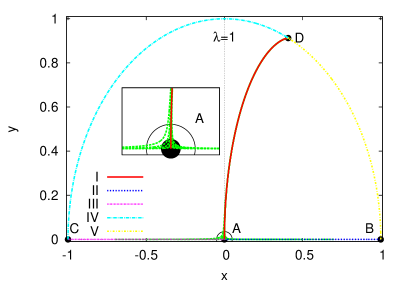
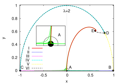
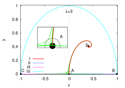
Figure 1: Structure of the phase space according to the dynamical system (4) in the case of $\lambda=\mathrm{const.}$ We show the critical points of Table 1 and the heteroclinic trajectories described in Sec. II that join them in each case, see text for details. Notice that the phase space is split in different disjoint regions for which the heteroclinic lines act as separatrices. Also shown are different trajectories in phase space obtained as numerical solutions of the dynamical system  (4), that depart from different points with $y_{i}=10^{-4}$. It can be seen that all trajectories are focused around the heteroclinic line I that connects the saddle point A (see the insets) with the corresponding stable point D or E in each case. The semicircle around the origin of coordinates corresponds to $\Omega_{\phi}=x^{2}+y^{2}=(0.05)^{2}$.

II.3 General dynamics for the exponential case

The general dynamics of a scalar field endowed with an exponential potential is completely described by the properties of the critical points and the heteroclinic lines of its phase space. Examples of different trajectories were given in Ref.Copeland et al. (1998). Here we will focus our attention only in trajectories that are consistent with an early perfect-fluid dominated Universe.

In Fig. 1 we also show examples of different trajectories departing closely from the perfect fluid domination point A. The general behavior of these particular trajectories can be quoted quite simply: each trajectory lies close to the heteroclinic line that joins the saddle perfect fluid-dominated point A and the stable critical point at hand in each case (see the heteroclinic lines I in all plots in Fig. 1). We can turn this quote into a stronger statement: the general dynamics of a cosmological scalar field endowed with an exponential potential, is well described by the heteroclinic trajectory that joins the perfect fluid dominated point with the late time attractor present in the phase space.

By studying this single trajectory, one can in principle determine the agreement of a given model, in the exponential case, with the expected evolution of the Universe. From the numerical point of view, the drawing of the heteroclinic trajectory needs of very especial initial conditions. It is not possible to find a full analytical solution for the heteroclinic trajectory we are interested in, but at least the behavior of the trajectory close to the origin of coordinates can be easily determined as follows.

We first write the linear equations of motion that are used to study the stability of critical points in autonomous systems. For the case of the perfect fluid-dominated point A, the linearization of the system (4) has the explicit solution

$$\left(\begin{array}[]{c}x\\ y\end{array}\right)=x_{i}\left(\begin{array}[]{c}1\\ 0\end{array}\right)e^{-3(2-\gamma)N/2}+y_{i}\left(\begin{array}[]{c}0\\ 1\end{array}\right)e^{3\gamma N/2}\,,$$ (11)

where we used the original phase space variables $(x,y)$ for the perturbations $(u,v)$, which is very convenient as the perturbation procedure is made around the origin of coordinates. Here, $x_{i}$ and $y_{i}$ refer to the initial values of the phase space variables.

For both cases of a relativistic and a pressureless fluid, the first eigenvalue is negative definite, $m_{1}=-3(2-\gamma)/2<0$, and then the kinetic energy of the scalar field must decrease for trajectories nearby the critical point A. On the other hand, the second eigenvalue is positive definite, $m_{2}=3\gamma/2>0$, and then the potential energy must increase. In terms of the dynamical system jargon, one says that the critical point A is a saddle point and its normal directions, represented by the eigenvectors of the stability matrix $\mathcal{M}$, see Eq. (9), coincide with those of the phase space axes, see Eq. (11).

We have learned then that the kinetic energy of the scalar field decreases if the latter is subdominant with respect to the perfect fluid, which is the expected situation in the early Universe. This also means that the kinetic variable $x$ must be smaller than the potential one $y$. If we now make a second order expansion of Eq. (4a), but still a first order expansion of Eq. (4b), around the same critical point A, we find

$$x^{\prime} = -\frac{3(2-\gamma)}{2}x+\lambda\sqrt{\frac{3}{2}}\,y^{2}\,,$$ (12a)

$$y^{\prime} = \frac{3\gamma}{2}y\,,$$ (12b)

whose general solutions, under the assumption that $\lambda$ is constant, are

$$x(N) = x_{i}e^{-3(2-\gamma)N/2}+\sqrt{\frac{2}{3}}\frac{\lambda}{(2+\gamma)}y^{2}\,,$$ (13a)

$$y(N) = y_{i}e^{3\gamma N/2}\,.$$ (13b)

It can be seen that, if we neglect the decaying solution, the kinetic energy evolves proportionally to the square of the potential energy, namely

$$x(y)=\frac{2}{(2+\gamma)}\frac{\lambda}{\sqrt{6}}y^{2}\,.$$ (14)

This is in good agreement with our assumption that the kinetic perturbation $x$ is one order of magnitude smaller than potential perturbation $y$. For future reference, we shall call Eq. (14) the thawing constraint. Notice that Eq. (14) has the same form as the famous slow-roll condition

$$3H\dot{\phi}\simeq-\partial_{\phi}V\quad\Rightarrow\quad x(y)=\frac{\lambda}{\sqrt{6}}y^{2}\,,$$ (15)

except for the correction induced by the presence of the perfect fluid through its EOS $\gamma$.

We have found the early behavior of the heteroclinic line that departs from the perfect fluid-dominated point, in the phase space the trajectory corresponds to the loci of a rotated parabola. Such a behavior can be easily seen in all lines I in Fig. 1; actually, the heteroclinic trajectories in Fig. 1 were found from the numerical solution of Eqs. (4) with initial conditions subjected to Eq. (14).

Eq. (14) can be written in the more recognizable terms of the flow parameter $F\equiv\gamma_{\phi}/(\Omega_{\phi}\lambda^{2})$, defined by Cahn, de Putter, and Linder in Ref.Cahn et al. (2008). If we take the thawing constraint (14) and the definitions in Eq. (7), we find that

$$F\simeq\frac{4}{3(2+\gamma)^{2}}\,,$$ (16)

and then we recover the known value $F=4/27$ if the dominant perfect fluid is pressureless matter $(\gamma=1)$, whereas $F=3/25$ if it is a relativistic fluid $(\gamma=4/3)$. In passing by, we note that the value of the flow parameter under the terms of the slow-roll condition (15) is $F=1/3$. The asymptotic values of some other quantities around the point $(0,0)$ can also be found, as for instanceLinder (2006); Cahn et al. (2008):

$$\frac{3H\dot{\phi}}{-\partial_{\phi}V}\simeq\frac{2}{2+\gamma}\,,\quad\frac{\ddot{\phi}}{\partial_{\phi}V}\simeq-\frac{\gamma}{2+\gamma}\,.$$ (17)

As we have said before, critical points in the exponential case are also fixed points, and then they seem to have more relevance that the trajectories themselves on phase space. This is true in the case of early and late time attractors, but particular trajectories are important if in addition one is interested in solutions which are in agreement with the stringent constraints arising from the radiation and matter dominated eras of the early Universe.

In Fig. 1 we show that trajectories with initial values close to the perfect fluid-dominated point A follow a quite similar path to that of the heteroclinic trajectory that connects point A with any of the stable fixed points at hand. The seemingly attractor character, or focusing property, of this heteroclinic line comes from a combination of the saddle properties of point A and the attractor character of the ending stable point. In the following sections, we will argue that this nice property is preserved in the case of general scalar field potentials.

III Dynamics of general scalar field models

In the case of an exponential potential, critical points are truly equilibrium fixed points. For the case $\lambda$ is also a variable, those points are not fixed, but they still represent, for a given value of $\lambda$, the points at which the 2-dim phase space velocity $(x^{\prime},y^{\prime})$ vanishes. In other words, the velocity field on the 2-dim phase space $(x,y)$ has the same structure than that in the exponential case, but now the location of the critical points can change as $\lambda$ evolves.

If $\lambda$ changes slowly, the critical points can be treated as if they were approximately fixed points; this feature is particularly useful in the case of quintessence fields, as one expects slow variations in the roll parameter $\lambda$ to have a solution with an accelerating expansion of the Universe at late times when the scalar field is the dominant component. However, the same can happen at early times, when the scalar field is subdominant with respect to the radiation and matter components. Hence, we expect the early and late time evolution of general scalar field models to proceed as in the case of the exponential potential, even though the intermediate-time dynamics of the scalar field may be more involved due to the evolution of the roll parameter $\lambda$.

III.1 Early dynamics of thawing and freezing scalar field solutions

From the dynamical system perspective, $\lambda$ plays an important role in determining the existence and stability properties of two important critical points: the scalar field dominated solution D and the scaling solution E, see Table 1. As we shall show, some aspects of the early and late time evolution of scalar fields can be understood if those two critical points are taken into account.

For simplicity, let us start with the assumption that $\lambda\ll 3\gamma$, and that $\lambda$ is a monotonic growing function of $N$ (this condition is not crucial for the argument, but it helps to visualize the description below). Thus, the scaling solution does not exist, and the only critical solution on the 2-dim phase space is that of scalar field domination, point D. If $\lambda$ changes slowly and keeps a value below $3\gamma$, the 2-dim velocity flow will focus the trajectories to that point, and then we shall recover a scalar field-dominated and accelerating Universe as long as $\lambda<\sqrt{2}$ at the present time.

Notice that we have just described the evolution expected for thawing solutions, in which the EOS starts very close to the cosmological constant value, $\gamma_{\phi}\simeq 0$, the flow parameter is $F=4/27$, and the field gains kinetic energy as its evolution proceeds in the form suggested by Eqs. (14). As the value of $\lambda$ grows, the scalar field-dominated point D moves clockwise and so does the phase space trajectory (see, for instance, Fig. 6 below).

Another extreme case is that in which $\lambda^{2}\gg 3\gamma$, and $\lambda$ is a monotonic decreasing function of $N$ (as before, this condition is not crucial for the argument, but it also helps to visualize the description below). For this case, the scalar field-dominated solution D does not exist, but the scaling solution E comes into play. For large values of $\lambda$, this latter critical point is located very close to the perfect fluid domination one, point A, see Table 1. Again, if the variation of $\lambda$ is slow enough, the field follows the heteroclinic trajectory that departs from the perfect fluid-dominated solution, hooks up with the scaling solution and follows it as the value of $\lambda$ changes. It should be stressed out here that we are referring to the same heteroclinic line described above for thawing fields and which is partially described by Eq. (14).

The scaling point E moves outwards from the origin in phase space if $\lambda$ decreases, and then $\gamma_{\phi}\simeq\gamma$ throughout this period; if at some point $\lambda^{2}<3\gamma$, then the scaling solution disappears and the scalar field then looks for the scalar field-dominated solution D. Contrary to the previous case, the trajectory of the scalar field moves counterclockwise in the phase space (see, for instance, Fig. 3 below). While the scalar field sits down on the scaling solution, we easily infer that the flow parameter is $F=1/3$, and then we have just described the evolution of freezing tracker fields.

We have seen that for a tracker solution we need the value of $\lambda$ to allow the appearance of the scaling solution close to the perfect fluid dominating solution, which is assured by asking $\lambda^{2}\gg 3\gamma$. For intermediate values $\lambda\sim 3\gamma$, the scaling solution may not exist or, if it exists, it is located far away from the origin of the phase space. Thus, the behavior in the proximity of the origin must be that of the thawing solution. However, notice that a purely thawing potential, for which $\lambda$ grows, will never be able to accelerate the expansion of the Universe at late times if initially $\lambda\sim 3\gamma$.

If the same is assumed for a purely freezing potential, for which $\lambda$ decreases, then the scalar field will anyway show a thawing behavior, because the scaling solution is never at hand for it to catch it up. The freezing potential has the chance to accelerate the expansion of the Universe, if $\lambda$ decreases fast enough as to fulfill the condition $\lambda<\sqrt{2}$ before the present time.

III.2 Geometric interpretation of the Flow parameter

There is a simple geometrical interpretation of the flow parameter $F$ in Eq. (16) in terms of trajectories in phase space. As we have said before, what we have called the thawing solution (14) indeed corresponds to the initial part of the heteroclinic trajectory that joins the (saddle) perfect fluid-dominated solution A to any of the stable solutions at hand. Most trajectories seem then to be focused towards the heteroclinic trajectory, and then the adjective flow is well deserved for the parameter $F$.

In the case of freezing behavior, we have shown that trajectories first engage with the thawing solution and then hook up with the scaling solution; in consequence, the flow parameter takes on the freezing value $F=1/3$. The flow now refers to the fact that solutions are following the scaling solution as it evolves outwards from the phase space origin. The focusing of the trajectories is achieved via the stability properties of the scaling solution.

III.3 The tracker theorem

The nice attractor features of freezing fields at early times come basically from its tracker nature, a term first applied to scalar fields in Ref.Zlatev et al. (1999). In this paper, the authors established a theorem for the necessary conditions for a scalar field to show tracking behavior; in simple terms, one needs at early times the tracker parameter to be nearly constant and to satisfy the condition $(\Gamma-1)>0$. One can though understand the tracker conditions in more simple terms by using the dynamical system equations (4).

We have seen that the attractor property of freezing fields arises because one sets up large initial values of the roll parameter $\lambda$, so that the scaling solution E is a critical point of the 2-dim phase space velocity $(x^{\prime},y^{\prime})$. The larger the value of $\lambda$, the easier is for the scalar field to catch up the scaling solution. From this point of view, the tracker condition just refers to large initial values of the roll parameter that allow the appearance of the scaling solution E. (As a curiosity, one can see that the attractor character of the tracker solution discussed in Ref.Zlatev et al. (1999) actually coincides with the analysis made in Ref.Copeland et al. (1998) for the scaling solution.)

However, one can go back to the usual tracker conditions if we take a look at the evolution equation of the roll parameter, Eq. (8). It can be seen that large initial values of the roll parameter are only allowed for scalar field models for which $\lambda$ is a growing function if we go backwards in time; that is, we need $(\Gamma-1)>0$. What we do not need is the slow variation of the tracker parameter, because, as we shall show in the numerical experiments of Sec. IV, the very condition $\lambda\gg 1$ leads to $x\to 0$. Hence, it is not the tracker parameter but the vanishing of the kinetic energy the responsible for the slow-variation of the roll parameter at early times, see Eq. (8). This enhances the possibilities of the scalar field to catch up the scaling solution, as the corresponding critical point on the 2-dim phase space $(x,y)$ moves adiabatically.

Therefore, the tracker theorem can be restated in simpler terms as follows. The tracker property appears for any scalar field model in which the roll parameter $\lambda$ is capable of taking on large initial values in the early Universe. It is easier to look at the expected evolution of $\lambda$, than to explore the more involved tracker parameter $\Gamma$, to determine the tracker properties of a given scalar field model.

III.4 Late time dynamics

The late time dynamics of the quintessence fields will depend upon its thawing or freezing behavior. In the case of thawing fields, we expect that they slowly deviate from the cosmological constant values, and that $\lambda$ moves from small to large values. If a thawing field is currently accelerating the expansion of the Universe, then $\lambda<\sqrt{2}$ today. It may be the case that $\lambda$ takes even larger values in the future, so that the quintessence field is not able to accelerate the cosmic expansion and can even provoke the appearance again of the scaling solution E on the phase space if at some point $\lambda^{2}>3\gamma$.

As for freezing fields, they start with large values of $\lambda$, but the latter has to migrate to smaller values $\lambda<\sqrt{2}$ so that the inflationary scalar field-dominated solution D appears on time. If this were also the trend for the future, we can only expect that a freezing field will only come closer to the cosmological constant behavior, i.e. $x\to 0$ and $y\to 1$, as $\lambda\to 0$.

Whether the field is thawing or freezing, its capability for providing an accelerating solution nowadays can be characterized in terms of $\lambda$, as it is only necessary that the (inflationary) scalar field dominated solution D becomes alive. Hence, nowadays $\lambda$ should be of the order of $\lambda^{2}\simeq 3(1+w_{\phi,0})$.

Even if the early dynamics of a scalar field resembles very much that of an exponential potential, the late-time dynamics can be more involved and strongly depends upon the explicit form of the scalar field potentialde la Macorra and Piccinelli (2000); Fang et al. (2009). Nonetheless, an easy description can be given for those cases in which Eqs. (4) and (8) together form a closed and autonomous system of equationsFang et al. (2009). For these cases, the phase space is truly 3-dimensional, $(x,y,\lambda)$, and we will refer to it hereafter as the augmented phase space. Notice that the heteroclinic lines I, II, and III described in Sec. II.2 retain its character for any value of $\lambda$; in geometric terms, we can see that the augmented phase space occupies, in general, the interior region of a unitary cylinder whose axis lies along the $\lambda$-direction.

If there is a value $\lambda_{\ast}$ such that $[\Gamma(\lambda_{\ast})-1]=0$, then there exist generalized scalar field-dominated and scaling solutions in the augmented phase space $(x,y,\lambda)$. The properties of these critical fixed points are quite similar to their exponential counterparts in Table 1 in that one only needs to make the replacement $\lambda\to\lambda_{\ast}$. Moreover, there also exists the generalized perfect fluid-dominated solution, which exists for any value $\lambda$ and is always a saddle point.

Whenever the generalized scalar field dominated D and scaling E solutions exist, there can be a unified description of the dynamics in terms again of the heteroclinic line that joins the perfect fluid dominated point A to the stable point available in the augmented phase space. As in the case of the exponential potential, the general solution for a given model is then characterized by such heteroclinic line. Even more, in our numerical experiments with different potentials in Sec. IV, we will find that the early description of the heteroclinic points is also given by the thawing behavior in Eq. (14). This was to be expected, as the evolution of $\lambda$ depends upon the second order perturbations of $x$, see Eq. (8), and then most of the motion around the perfect fluid-dominated solution must proceed at $\lambda\simeq\mathrm{const.}$

There is though a non-trivial difference with respect to the exponential case: the de Sitter point $(0,1)$ exists as a late time attractor if $\lambda\to 0$ and $[\Gamma(0)-1]>0$. That is, for any scalar field model in which the roll parameter vanishes at late times the final fate is the cosmological constant casede la Macorra and Piccinelli (2000); Fang et al. (2009).

IV Numerical examples

We now present some numerical solutions of the EKG equations in cases in which Eqs. (4) and (8) form a closed and autonomous system of equations. This is done for numerical purposes, as in other more general cases we may need to write a full hierarchy of equations for higher derivatives of the scalar field potential. As we have discussed before, it will be only necessary to look at the properties of the 2-dim phase space $(x,y)$ to have an ample picture about the dynamics of scalar fields.

IV.1 Monotonic freezing case

As a typical example for a freezing model we take the tracker models $V(\phi)=M^{4+n}\phi^{-n}$, with $n>0$, for which the roll parameter and the tracker parameter are, respectively, $\lambda=n/(\kappa\phi)$ and $\Gamma-1=1/n>0$; notice that this is a monotonic freezing case, as the latter condition on the tracker parameter means that the roll parameter is an always decreasing function. In fact, the equation of motion of the roll parameter is

$$\lambda^{\prime}=-\frac{\sqrt{6}}{n}x\lambda^{2}\,,$$ (18)

and then it is one of those fortunate cases in which the equations of motion (4) and (18) together form an autonomous system of equations, which is able to represent the full dynamics of the original EKG system.

According to the phase space analysis in previous sections, this type of models have the following fixed points in the augmented phase space on the plane $\lambda=0$: perfect fluid-dominated point A, kinetic dominated points B and C, and the de Sitter point $(0,1)$. In addition, points D and E are also critical, but not fixed, points at different slices with $\lambda=\mathrm{const.}$ Even though we cannot apply here the stability analysis of Ref.Fang et al. (2009), we expect the de Sitter point to be a stable point: once the field is rolling down its potential we have $x>0$, and then $\lambda$ should be an ever decreasing function according to Eq. (18). In this form, the system must approach the de Sitter point asymptotically.

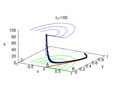
Figure 2: Numerical solutions of Eqs. (4) and (18), for numerical convenience we chose $n=50$. Shown are the trajectories (black-solid and blue-dotted lines) in the 3D phase space $(x,y,\lambda)$ for different initial conditions of the system (4) and (18). The corresponding projections onto the $(x,y)$ plane are also shown (red-solid and green-dashed lines); see the text and Fig. 3 for a comprehensive description of the dynamics on the $xy$-plane.

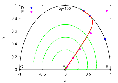
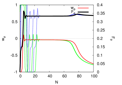
Figure 3: Numerical solutions of Eqs. (4) and (18), which together form an autonomous dynamical system; for numerical convenience we chose $n=50$. (Top) Trajectories of the numerical solutions on the 2-dim $(x,y)$ plane. The dots denote the positions of the critical points D and E, see Table 1, as $\lambda$ evolves. All the solutions initially have $\lambda_{i}=100$. In particular, the (red solid) line is the heteroclinic line that joins the perfect fluid-dominated point A with the de Sitter point $(0,1)$. (Bottom) The evolution of the scalar field EOS $w_{\phi}$ (red-solid and green-dashed lines) and the flow parameter $F$ (black-solid and blue-dotted lines) for the same numerical solutions as in the top figure. Both parameters show a tracker intermediate behavior for which $w_{\phi}\simeq\mathrm{const.}$ and $F=1/3$. At late time, the EOS takes on negative values as the solution evolves towards the de Sitter point and enters a pure slow-roll regime with $F\to 1/3$ again, see Eq. (15).

Numerical solutions of the set of Eqs. (4) and (18) are given in Figs. 2 for the 3-dim phase space $(x,y,\lambda)$, and in Fig. 3 for the 2-dim phase space $(x,y)$, for $n=50$. A detailed description of the behavior of the different curves is as follows. The attractor trajectory is the heteroclinic line that joins the saddle point A $(0,0)$ with the stable de Sitter point $(0,1)$; the behavior of this heteroclinic line in the neighborhood of point A is given by the thawing solution (14). Because of the large initial value of the roll parameter, $\lambda_{i}=100$, the scaling solution, point E, is present. The heteroclinic trajectory hooks up with the scaling point, and the latter moves outwards as the value of $\lambda$ decreases. Once $\lambda<\sqrt{6}$, there also appears the scalar field dominated solution, point D, which starts to move counterclockwise on the unitary circumference as $\lambda$ continues decreasing. Both critical points merge once $\lambda=3\gamma$ and the scaling point formally disappears, and the motion of the heteroclinic line is now guided by the still moving point D until they reach together the de Sitter point.

The description we have given for the heteroclinic line suffices to understand the general behavior of inverse power-law potentials. To show the attractor feature of the heteroclinic line, we have also solved the equations of motion for diverse initial conditions $(x_{i},y_{i})$ but keeping the same $\lambda_{i}=100$. It is clear that the curves follow the heteroclinic line at late times, as expected. But for this type of potentials we notice a peculiar early behavior denoted by the clockwise semi-circumferences. This behavior is easily explained if we write the equations of motion (4) in the limit $\lambda\gg 1$, and then

$$x^{\prime}\simeq\lambda\sqrt{\frac{3}{2}}y^{2}\,,\quad y^{\prime}\simeq-\lambda\sqrt{\frac{3}{2}}xy\,.$$ (19)

It can be shown that, under these equations, the scalar field density parameter (7) is a conserved quantity, i.e. $\Omega_{\phi}=x^{2}+y^{2}=\mathrm{const.}$, and then the phase space variables should move clockwise on circumferences until they lose enough potential energy ($y\to 0$) and the scalar field energy is dominated by its kinetic component (there is no other option, anyway, as the variable $y$ cannot become negative because of the heteroclinic separatrix $(x,y=0)$). The clockwise motion is explained by the fact that the field prefers to move downhill its potential, $x>0$, rather than otherwise. We finally note that the circular motion occurs quite rapidly, an estimation can be made from Eqs. (19), and then the $e$-fold interval for the circular motion is $\Delta N\sim 1/\lambda$.

In Fig. 3 we also make a translation of the scalar field dynamics in terms of the scalar field EOS $w_{\phi}=\gamma_{\phi}-1$ (see Eq. (7)) and the flow parameter $F$ (see Eq. (16)). The scalar field EOS reaches a tracker regime that almost perfectly traces the background EOS, which is $\gamma=1$ for the numerical examples; this is actually the tracker behavior described in detail in Ref.Zlatev et al. (1999). The small difference between the two EOS means that the scalar field redshifts a bit slower than the background field. This difference, even if small, is important for the later overtaking of the background dynamics by the scalar field. The value of $w_{\phi}$ asymptotically approaches the de Sitter value, $w_{\phi}\to-1$.

As for the flow parameter, its value in the tracker regime is the expected one, $F=1/3$, which is a constant value for almost the whole evolution. There is small ’bump’ at the transition point at which the solution leaves the tracker regime, but $F_{\phi}\to 1/3$ asymptotically again, signaling that the scalar field is entering into a pure slow-roll regime at late times, see Eq. (15).

As the heteroclinic trajectory is a strong attractor, it suffices to scan the form of heteroclinic trajectories in phase space for different initial values of $\lambda$ in order to find physically acceptable accelerating solutions, as is made in Fig. 4. We can see that the initial value of $\lambda$ should be small enough so that the heteroclinic line can provide of physical parameters in agreement with cosmological observations. According to Fig. 4, it is necessary to have $\lambda_{i}<0.5$ if we want heteroclinic trajectories to be inside the arc of radius $\Omega_{\phi}=0.7$ and angles corresponding to $-1<w_{\phi}<-0.94$.

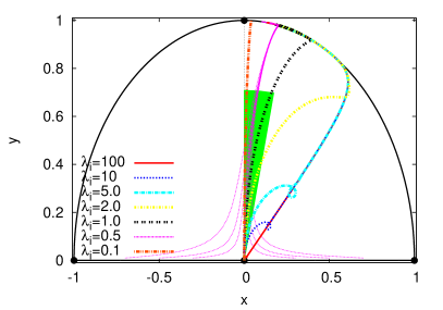
Figure 4: Heteroclinic lines departing from the perfect fluid-dominated point A, that were obtained from the numerical solutions of Eqs. (4) and (18). For each case, the initial conditions for $x$ and $y$ were chosen according to the thawing constraint (13). The shaded region is a circular arc of radius $\Omega_{\phi}=0.7$ and angles corresponding to $-1<w_{\phi}<-0.94$. It can be seen that only heteroclinic lines with $\lambda_{i}\leq 0.5$ may be able to provide of a physically viable accelerating Universe.

IV.2 Monotonic thawing case

To study the general behavior of thawing models, we may use the example of a PNGB potential of the form $V(\phi)=M^{4}\cos^{2}(\alpha\kappa\phi)$, where $\alpha$ is a free parameter of the modelDutta and Scherrer (2008). The roll and tracker parameters for this kind of potentials are

$$\lambda=2\alpha\tan(\alpha\kappa\phi)\,,\quad\Gamma(\lambda)=-\frac{1}{2}\left(1+\frac{2\alpha^{2}}{\lambda^{2}}\right)\,.$$ (20)

The PNGB potential is a representative case of a monotonic thawing case, for which the roll parameter is always an increasing function. However, we should remember that the PNGB potential has a zero minimum at $\alpha\kappa\phi=\pi/2$, and it is at this point that the roll parameter diverges, $\lambda\to\infty$; hence, the autonomous dynamical system cannot describe the dynamics of the scalar field model beyond this point. This is a caveat of the dynamical system approach that appears for any model with a zero minimum, see for instanceUrena-Lopez and Reyes-Ibarra (2009); Matos et al. (2009).

Some other models without a minimum in the potential can be chosen from the examples in the specialized literature. We shall use a generic example in which the representative features of monotonic thawing potentials appear acutely. We write Eq. (8) in the form

$$\lambda^{\prime}=\frac{\sqrt{6}}{n}x\lambda^{2}\,,$$ (21)

which also arises in the case of power law potentials $V\sim\phi^{n}$. We have verified that other monotonic thawing potentials display qualitatively the same generic behavior of this example (seede la Macorra and Piccinelli (2000) for some other instances).

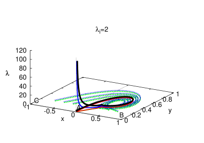
Figure 5: Numerical solutions of Eqs. (4) and (18), for numerical convenience we chose $n=20$. Shown are the trajectories (black-solid and blue-dotted lines) in the 3-dim phase space $(x,y,\lambda)$ for different initial conditions of the system (4) and (21). The corresponding projections onto the $(x,y)$ plane are also shown (red-solid and green-dashed lines); see the text and Fig. 6 for a comprehensive description of the dynamics on the $xy$-plane.

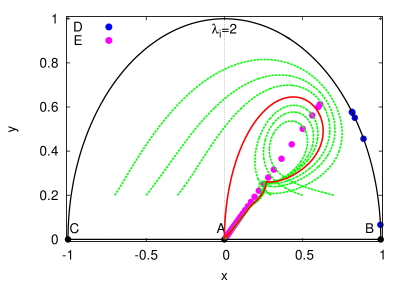
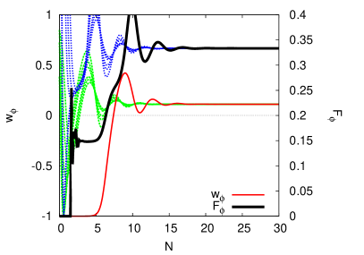
Figure 6: Numerical solutions of Eqs. (4) and (21), which together form an autonomous dynamical system; for numerical convenience we chose $n=20$. (Top) Trajectories of the numerical solutions on the 2-dim $(x,y)$ plane. The dots denote the positions of the critical points D and E, see Table 1, as $\lambda$ evolves. All the solutions initially have $\lambda_{i}=2$. In particular, the (red solid) line is the homoclinic line that joins the perfect fluid-dominated point A with itself. (Bottom) The evolution of the scalar field EOS $w_{\phi}$ (red-solid and green-dashed lines) and the flow parameter $F$ (black-solid and blue-dotted lines) for the same numerical solutions as in the top figure. Both parameters show an early thawing behavior for which $w_{\phi}\simeq-1$ and $F=4/27$. At late times, the EOS takes on positive values as the solution evolves back to the point $(0,0)$ and $F\to 1/3$.

As in the case of freezing models, thawing potentials has the following fixed points in the augmented phase space on the plane $\lambda=0$: perfect fluid-dominated point A, kinetic dominated points B and C, and the de Sitter point $(0,1)$. In addition, points D and E are also critical, but not fixed, points at different slices with $\lambda=\mathrm{const.}$ Contrary to the freezing case, we expect the de Sitter point to be an unstable point: once the field is rolling down its potential we have $x>0$, and then $\lambda$ should be an ever increasing function according to Eq. (21). This latter fact has another undesirable consequence for thawing models: there is not a fixed critical point that can act as a late-time attractor. Thus, the thawing solution we have found before in the neighborhood of the perfect fluid-dominated solution, see Eq. (13), is no longer part of a heteroclinic line, but now we have the presence of a homoclinic line only, that eventually connects a critical point with itself.

Numerical solutions of the set of Eqs. (4) and (21) are given in Fig. 5 for the 3-dim phase space $(x,y,\lambda)$, and in Fig. 6 for the 2-dim phase space $(x,y)$; in all cases $\lambda_{i}=2$. The same features appear in both Figs. 3, and 6, so that a quick comparison can be made of the thawing case with the freezing case.

First of all, we cannot notice any kind of strong attractor trajectory on the phase space at early times as it is the case in freezing models. This was anticipated above because there is only a homoclinic trajectory departing from and eventually arriving at the (saddle) perfect fluid-dominated point; in practice, the homoclinic line is a closed loop. The departing behavior of the loop is given by the thawing condition (13), but the late time behavior is dictated by the scaling solution E as $\lambda\to\infty$. The homoclinic trajectory, however, do split the $(x,y)$ in two parts, as trajectories departing at $x<0$ ($x>0$) surround the loop in the clockwise direction by its outside (inside) part as they approach the scaling solution E at late times.

In terms of physical variables, we notice that the scalar field EOS for the homoclinic line departs from $w_{\phi}\simeq-1$, and ends up with a constant value at late times which is a bit stiffer than the background EOS (in this example $\gamma=1$). As for the flow parameter, we notice the expected thawing behavior at early times, $F=4/27$, but also the freezing one at late times, $F=1/3$.

Even though the homoclinic trajectory is not a strong attractor, it anyway determines the way other arbitrary trajectories wander about on the phase space. Thus, in order to search for valid accelerating solutions, it suffices to scan the form of homoclinic trajectories in phase space for different initial values $\lambda_{i}$. This is actually shown in Fig. 7. For small enough values of $\lambda$, the homoclinic trajectory reaches the unitary circle because of the presence of the scalar field-dominated point D. Remember that this critical point exists for $\lambda^{2}<6$ and is stable for $\lambda^{2}<2$. We also show in Fig. 7 the homoclinic trajectories that remain within the arc of radius $\Omega_{\phi}=0.7$ and angles corresponding to $-1<w_{\phi}<0.94$; these trajectories could provide a valid accelerating Universe at the present time.

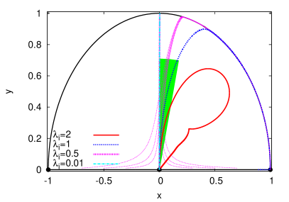
Figure 7: Homoclinic lines departing from the perfect fluid-dominated point A, that were obtained from the numerical solutions of Eqs. (4) and (21). For each case, the initial conditions for $x$ and $y$ were chosen according to the thawing constraint (13). The shaded region is a circular arc of radius $\Omega_{\phi}=0.7$ and angles corresponding to $-1<w_{\phi}<-0.94$. It can be seen that only homoclinic lines with $\lambda_{i}\leq 0.5$ may be able to provide of a physically viable accelerating Universe.

V Conclusions

We have given evidence for the existence of an unified description for the dynamics of general scalar field models, in terms of the heteroclinic trajectory that connects the perfect fluid-dominated stage of the Universe with any of the late-time attractors at hand in the phase space of the scalar field variables.

The numerical results shown in Figs. 4 and 7 strongly suggest that, in the case of single field models with a monotonic evolution of the roll parameter $\lambda$, the field should start in a thawing regime far away from the tracker one if it is to be consistent with an accelerating Universe at late times. Actually, the tracker regime seems to spoil in all cases the viability of quintessence models even if its early-time attractor properties are very appealingZlatev et al. (1999); Wang et al. (2011).

However, the early thawing behavior is a problematic one, as it requires special initial conditions, in particular, small initial values of the roll parameter $\lambda$. Moreover, as in the case of an exponential potentialCopeland et al. (1998), the initial value of the quintessence parameter $\Omega_{\phi}$ must be extremely small in order to be consistent with cosmological constraints and to prevent quintessence domination well before the present time. As for the late time dynamics, the approach presented here suggests that the roll parameter $\lambda$ is small at late times, and that its value should be related to the present value of the dark energy EOS by $\lambda^{2}\simeq 3(1+w_{0})$; in other words, the derivative of the quintessence potential must be related to the actual value of the dark energy EOS.

It is interesting to note that the aforementioned difficulties for thawing and freezing scalar fields are actually well known from the case of an exponential potentialCopeland et al. (1998). They are actually present in more general cases because the phase space equations of motion preserve its form in the general case, and then quintessence fields inherit the difficulties of the exponential case.

There is still the possibility of having single field models with a non-monotonic evolution of the roll parameter, in which the strong attractor properties of freezing fields can be combined with the appropriate late-time dynamics of thawing fields. This can in principle be achieved with the use of very contrived potentials (see an early example inZlatev et al. (1999)), in the case in which the roll parameter changes stochastically, or even in the case in which phase space dynamics needs a full hierarchy of equations of motionChongchitnan and Efstathiou (2007).

In any case, our general suggestion in the study of scalar field models is still the same. One should look for the heteroclinic line departing from the perfect fluid-domination point; this single trajectory encloses in itself enough information to determine the capabilities of the given quintessence field to act as a realistic dark energy model.