CDF/PUB/SEC_VTX/PUBLIC/10631
FERMILAB-TM-2515-E-PPD
An artificial neural network based $b$ jet identification algorithm at the CDF Experiment

Abstract

We present the development and validation of a new multivariate $b$ jet identification algorithm (“$b$ tagger”) used at the CDF experiment at the Fermilab Tevatron. At collider experiments, $b$ taggers allow one to distinguish particle jets containing $B$ hadrons from other jets. Employing feed-forward neural network architectures, this tagger is unique in its emphasis on using information from individual tracks. This tagger not only contains the usual advantages of a multivariate technique such as maximal use of information in a jet and tunable purity/efficiency operating points, but is also capable of evaluating jets with only a single track. To demonstrate the effectiveness of the tagger, we employ a novel method wherein we calculate the false tag rate and tag efficiency as a function of the placement of a lower threshold on a jet’s neural network output value in $Z+1$ jet and $t\bar{t}$ candidate samples, rich in light flavor and $b$ jets, respectively.

1 Introduction

The identification of jets originating from $b$ quarks is an important part of many analyses at high-energy physics colliders. Searches for the Higgs boson and measurements of top-quark properties depend on the ability to identify $b$ jets properly. Furthermore, in many new physics models, the third generation holds a special role, and therefore final states with $b$-quark jets are common. The high momentum of $B$ hadrons coupled with their long lifetimes result in a large distance between the interaction point and the decay vertex of the $B$ hadron (decay length). Additionally, a significant fraction ($\approx$20%) of $B$ hadrons decay with a soft lepton, i.e., a charged lepton with a few GeV of momentum. These qualities are key to distinguishing $b$-quark jets from other types of jets.

Almost all information as to whether or not a given jet originates from a $B$-hadron decay is carried in the tracks its charged particles leave in the detector. There are a few salient features of $B$-hadron decays which can be searched for via the tracks in a jet. The lifetime of a $B^{0}$ ($B^{\pm}$, $\Lambda_{b}$) hadron is 1.52 ps (1.64 ps, 1.42 ps). The distances these particles travel during their lifetimes can be resolved by the CDF tracking system, and it is therefore possible to identify the delayed decay of a $B$ hadron through the displacement of individual tracks with respect to the primary interaction point (the primary vertex) and also through the combining of tracks in the form of a fitted secondary decay vertex. Due to the large mass of the $b$ quark, the decay products of $B$ hadrons will form a larger invariant mass than those of hadrons not containing $b$ quarks. Furthermore, the large relativistic boost typical of a $B$ hadron will result in decay products which tend to be more energetic and collimated within a jet cone than other particles. Finally, particle multiplicities tend to be different for jets containing $B$-hadron decays compared to other jets; in particular, muons and electrons appear in approximately 20% of jets containing a $B$ hadron, typically either directly via semileptonic decay of the $B$ or indirectly through the semileptonic decay of a $D$ or $\Lambda_{c}$ resulting from a $B$ decay.

Many algorithms used at CDF were instrumental in the 1995 discovery of the top quark [1]. Here we review the standard $b$-tagging algorithms used at CDF. Similar techniques as those described in this paper have been developed at the D0 experiment [2] and at the CMS and ATLAS experiments at the LHC [3, 4].

SecVtx [5] is a secondary vertex tagger. It is the most commonly used $b$ tagger at CDF. Using only significantly displaced tracks that pass certain quality requirements within each jet’s cone, an iterative method is used to fit a secondary vertex within the jet. Given the relatively long lifetime of the $B$ hadron, the significance of the two-dimensional decay length $L_{\text{xy}}$ in the $r$-$\phi$ plane is used to select $b$-jet candidates. The algorithm can be performed with different sets of track requirements and threshold values. In practice, three operating points are used, referred to as “loose”, “tight”, and “ultra tight”.

The jet probability [6] tagger on the other hand does not look for a secondary vertex, but instead uses the distribution of the impact parameter significance of tracks in a jet, where impact parameter significance is defined as the impact parameter divided by its measured uncertainty ($d_{0}/\sigma_{d_{0}}$). By comparing these values to the expected distribution of values from light jets, it is possible to determine the fraction of light jets whose tracks would be more significantly displaced from the primary vertex than those of the jet under study. While light-flavor jets should yield a fraction uniformly distributed from 0 to 1, due to the long $B$ lifetime, $b$ jets often produce significantly displaced tracks and hence tend toward a fraction of 0. Although this algorithm produces a continuous variable for discriminating $b$ jets, in practice only three operating points are supported (jet probability $<$ 0.5%, 1%, and 5%).

Soft-lepton taggers [7] take a different approach to $b$ tagging. Rather than focusing on tracks within a jet, they identify semi-leptonic decays by looking for a lepton matched to a jet. The branching ratio of approximately 10% per lepton makes this method useful; however, if used alone, this class of tagger is not competitive with the previously mentioned taggers. Because a soft-lepton tagger does not rely on the presence of displaced tracks or vertices, it has a chance to identify $b$ jets that the other methods cannot. In practice in CDF only the soft muon tagger is used since high-purity electron or tau identification within jets is very difficult.

Neural networks (NNs) can use as many flavor discriminating observables as is computationally feasible; hence the efficiency of NN taggers is often equal to or greater than that of conventional taggers for a given purity. One such NN-based algorithm at CDF, called the “KIT flavor separator” [8], analyzes SecVtx-tagged jets and identifies secondary vertices that are likely from long-lived $B$ hadrons, separating them from jets with secondary vertices that originate from charm hadrons or that are falsely reconstructed. This flavor separator has been used in many CDF analyses, notably in the CDF observation of single top quark production [9]. Another NN-based algorithm, the “Roma tagger” [10, 11], has been used at CDF in light Higgs searches. While the SecVtx tagger attempts to find exactly one displaced vertex in a jet, the Roma tagger uses a vertexing algorithm that can find multiple vertices, as may be the case when multiple hadrons decay within the same jet cone (for example, in a $B\rightarrow D$ decay). Three types of NNs are used: one to distinguish heavy from light vertices, another to distinguish heavy-candidate from light-candidate unvertexed tracks, and a third that takes as inputs the first two NN outputs along with other flavor discriminating information, including SecVtx and jet probability tag statuses, number of identified muons, and vertex displacement and mass information. The performance of the Roma tagger is roughly equivalent to SecVtx at its operating points but allows for an “ultra loose” operating point yielding greater efficiency, useful in certain analyses.

In this paper we describe a new tagger that builds on the development of these taggers using feed-forward NN architectures. The NNs provide the ability to exploit correlations in many variables. The tagger is unique in its emphasis on individual tracks, and in its ability to evaluate jets with only a single track. Each track’s potential for having come from a $B$-hadron decay is evaluated by a NN, and the outputs of this NN are fed into a jet-wide NN along with other jet observables such as the significance of the displacement of the secondary vertex. The output of this NN, which we call the jet $b$ness, is designed to identify jets containing a $B$-hadron decay. The continuity of the NN output value allows for a tunable operating point corresponding to the desired purity and efficiency.

To characterize the tagger’s performance, the efficiency and mistag rate are obtained as a function of the jet $b$ness cut in $Z+1$ jet (rich in light flavor jets) and $t\bar{t}$ (rich in $b$ jets) candidate samples. This choice of data samples differs from many previous evaluations of performance using generic di-jet samples. The large data sample accumulated at the Tevatron allow us to use the more pure top quark samples for $b$ tagging efficiency studies. The ultimate use of this tagger is aimed at searches for standard model dibosons and Higgs bosons. The momentum spectrum of $b$ quarks in top pair production is better matched to these searches than the relatively soft quark momentum spectrum found in generic di-jet samples. Finally, since our tagger will incorporate information from many different tagging methods, techniques that, for instance, use soft lepton-tagged jets as an input to an efficiency measurement for displaced-vertex taggers cannot be used.

2 The CDF Detector

The CDF II detector is described in detail elsewhere [12]. The detector is cylindrically symmetric around the proton beam line with tracking systems that sit within a superconducting solenoid which produces a $1.4$ T magnetic field aligned coaxially with the $p\overline{p}$ beams. The Central Outer Tracker (COT) is a $3.1$ m long open cell drift chamber which performs 96 track measurements in the region between $0.40$ and $1.37$ m from the beam axis, providing coverage in the pseudorapdity region $|\eta|\leq 1.0$ [13]. Sense wires are arranged in eight alternating axial and $\pm 2^{\circ}$ stereo “superlayers” with 12 wires each. The position resolution of a single drift time measurement is about $140~{}\mu$m.

Charged-particle trajectories are found first as a series of approximate line segments in the individual axial superlayers. Two complementary algorithms associate segments lying on a common circle, and the results are merged to form a final set of axial tracks. Track segments in stereo superlayers are associated with the axial track segments to reconstruct tracks in three dimensions.

The efficiency for finding isolated high-momentum tracks is measured using electrons from $W^{\pm}\rightarrow e^{\pm}\nu$ decays identified in the central region $|\eta|\leq 1.1$ using only calorimetric information from the electron shower and the missing transverse energy. In these events, the efficiency for finding the electron track is $99.93^{+0.07}_{-0.35}\%$, and this is typical for isolated high-momentum tracks from either electronic or muonic $W$ decays contained in the COT. The transverse momentum resolution of high-momentum tracks is $\delta p_{T}/p_{T}^{2}\approx 0.1\%\,({\rm GeV}/c)^{-1}$. Their track position resolution in the direction along the beam line at the origin is $\delta z\approx 0.5$ cm, and the resolution on the track impact parameter, the distance from the beam line to the track’s closest approach in the transverse plane, is $\delta d_{0}\approx 350~{}\mu$m.

A five layer double-sided silicon microstrip detector (SVX) covers the region between $2.5$ to $11$ cm from the beam axis. Three separate SVX barrel modules along the beam line cover a length of 96 cm, approximately 90% of the luminous beam interaction region. Three of the five layers combine an $r$-$\phi$ measurement on one side and a $90^{\circ}$ stereo measurement on the other, and the remaining two layers combine an $r$-$\phi$ measurement with small angle stereo at $\pm 1.2^{\circ}$. The typical silicon hit resolution is 11 $\mu$m. Additional Intermediate Silicon Layers (ISL) at radii between 19 and 30 cm from the beam line in the central region link tracks in the COT to hits in the SVX.

Silicon hit information is added to COT tracks using a progressive “outside-in” tracking algorithm in which COT tracks are extrapolated into the silicon detector, associated silicon hits are found, and the track is refit with the added information of the silicon measurements. The initial track parameters provide a width for a search road in a given layer. Then, for each candidate hit in that layer, the track is refit and used to define the search road into the next layer. This stepwise addition of precision SVX information at each layer progressively reduces the size of the search road, while also accounting for the additional uncertainty due to multiple scattering in each layer. The search uses the two best candidate hits in each layer to generate a small tree of final track candidates, from which the tracks with the best $\chi^{2}$ are selected. The efficiency for associating at least three silicon hits with an isolated COT track is $91\pm 1\%$. The extrapolated impact parameter resolution for high-momentum outside-in tracks is much smaller than for COT-only tracks: $30~{}\mu$m, including the uncertainty in the beam position.

Outside the tracking systems and the solenoid, segmented calorimeters with projective geometry are used to reconstruct electromagnetic (EM) showers and jets. The EM and hadronic calorimeters are lead-scintillator and iron-scintillator sampling devices, respectively. The central and plug calorimeters are segmented into towers, each covering a small range of pseudorapidity and azimuth, and in full cover the entire $2\pi$ in azimuth and the pseudorapidity regions of $|\mathrm{\eta}|$$<$1.1 and 1.1$<$$|\mathrm{\eta}|$$<$3.6 respectively. The transverse energy $E_{T}$, where the polar angle is calculated using the measured $z$ position of the event vertex, is measured in each calorimeter tower. Proportional and scintillating strip detectors measure the transverse profile of EM showers at a depth corresponding to the shower maximum.

High-momentum jets, photons, and electrons leave isolated energy deposits in contiguous groups of calorimeter towers which can be summed together into an energy cluster. Electrons are identified in the central EM calorimeter as isolated, mostly electromagnetic clusters that also match with a track in the pseudorapidity range $|\eta|<1.1$. The electron transverse energy is reconstructed from the electromagnetic cluster with precision $\sigma(E_{T})/E_{T}=13.5\%/\sqrt{E_{T}({\rm GeV})}\oplus 2\%$, where the $\oplus$ symbol denotes addition in quadrature. Jets are identified as a group of electromagnetic and hadronic calorimeter clusters using the jetclu algorithm [14] with a cone size of 0.4. Jet energies are corrected for the calorimeter non-linearity, losses in the gaps betwen towers, multiple primary interactions, the underlying event, and out-of-cone losses [15]. The jet energy resolution is approximately $\sigma_{E_{T}}=1.0~{}{\rm GeV}+0.1\times E_{T}$

Directly outside of the calorimeter, four-layer stacks of planar drift chambers detect muons with $p_{T}>1.4~{}$GeV$/c$ that traverse the five absorption lengths of the calorimeter. Farther out, behind an additional 60 cm of steel, four layers of drift chambers detect muons with $p_{T}>2.0~{}$GeV$/c$. The two systems both cover a region of $|\eta|\leq 0.6$, though they have different structure and their geometrical coverages do not overlap exactly. Muons in the region between $0.6\leq|\eta|\leq 1.0$ pass through at least four drift layers lying in a conic section outside of the central calorimeter. Muons are identified as isolated tracks in the COT that extrapolate to track segments in one of the four-layer stacks.

3 Description of the neural network

All neural networks are trained using simulated data samples. The geometric and kinematic acceptances are obtained using a geant-based simulation of the CDF II detector [16]. For the comparison to data, all sample cross sections are normalized to the results of NLO calculations performed with the mcfm v5.4 program [17] and using the cteq6m parton distribution functions [18].

3.1 Basic track selection

A great deal of information as to whether a jet contains a $B$-hadron decay is contained within the jet’s individual tracks. Indeed, as described earlier, the jet probability algorithm [6] uses information solely based on the significance of the impact parameters of tracks. Furthermore, an important choice to make when seeking displaced vertices is which tracks to use as candidates for a fit. In light of this, our tagger takes a ground-up approach where the first step in the evaluation of how $b$-like a jet is involves using a neural network to discriminate $B$-hadron decay tracks from other tracks in a jet. We use relatively loose criteria when selecting which tracks to evaluate with our track-by-track NN, thereby improving the $b$-tagging efficiency. We reject tracks that use hits only in the COT, as the COT alone has insufficient resolution to distinguish the effects of the displacement of a $B$-hadron decay from the primary vertex. Additionally, a track must have a $p_{T}>0.4~{}\mathrm{GeV}/c$, a requirement CDF maintains for all tracks, and be found within a cone of $\Delta R<$ 0.4 about the jet axis, where $\Delta R=\sqrt{(\Delta\phi)^{2}+(\Delta\eta)^{2}}$. Finally, for tracks within a jet, track pairs are removed if they are oppositely charged, form an invariant mass within 10 MeV of that of a $K_{S}$ (0.497 GeV$/c^{2}$) or $\Lambda$ (1.115 GeV$/c^{2}$), and can be fit into a two-track vertex. This requirement is included to reject non-$b$ jets that contain these long-lived particles, as they can mimic $b$ jets, compromising our purity.

3.2 The track neural network

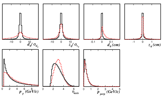
Figure 1: Inputs used in the neural network for calculating the per-track $b$ness. The red dashed line is signal and the black solid line is background. The $y$-axis is in arbitrary units.

The two primary categories of input variables to the track-by-track NN are observables related to the displacement of the track from the primary vertex and observables related to the kinematics of the track. The former category includes the track’s signed impact parameter ($d_{0}$), its $z$ displacement ($z_{0}$) from the primary vertex, and the significances of these two quantities, given their uncertainties ($d_{0}/\sigma_{d_{0}}$ and $z_{0}/\sigma_{z_{0}}$). The latter category takes advantage of the fact that tracks from $B$-hadron decays have a somewhat harder $p_{T}$ spectrum than other tracks, and are more collimated within a jet. This category includes the track’s $p_{T}$, its pseudorapidity ($\eta_{\text{axis}}$) with respect to the jet axis, and its momentum ($p_{\text{perp}}$) perpendicular to the jet axis.

A final input variable to the track-by-track $b$ness NN is the $E_{T}$ of the jet, since distributions of the track observables are correlated with their parent jet $E_{T}$. To ensure that the distributions of track observables used to train the track-by-track NN are not kinematically biased, $B$ hadron and non-$B$ hadron tracks are weighted in training to have the same parent jet $E_{T}$ distribution.

Figure 1 shows distributions of the track variables in pythia [19] $ZZ\rightarrow jjjj$ Monte Carlo simulations (MC) for tracks matched by $\Delta R<0.141$ to particles that come from $B$-hadron decays compared to tracks in jets which are not matched to $B$ hadrons. These figures indicate that the displacement variables tend to give more discrimination power than the kinematic variables; in particular, the impact parameter variables are the most important inputs to the NN.

The NN is a feed-forward multilayer perceptron with a single output and two hidden layers of 15 and 14 nodes implemented using the MLP algorithm from the TMVA package [20]. The same number of signal and background events was used in the training. The performance of the NN was similar with larger numbers of hidden layer nodes.

3.3 The jet neural network

To determine how $b$-like a jet is, we train a NN to distinguish jets containg $B$-hadron decays from those not containing $B$-hadron decays. Many of the input variables come directly from the track-by-track NN described in the previous section: the NN values of the five most $b$-like tracks ($b_{i}$, $i=0..4$), as well as the number ($n_{\text{trk}}$) of tracks with a NN output greater than 0.

We use tracks with track-by-track NN values greater than -0.5 in the fitting of a secondary vertex. An initial fit is performed with all such tracks; if the largest contribution to the total fit $\chi^{2}$ from any of them exceeds a value of 50, it is removed, and the remaining tracks are re-fit. This process continues until either the largest $\chi^{2}$ contribution from any track is less than 50, or there are fewer than two tracks to be fit. If a secondary vertex is successfully fit, then the significance of its displacement from the primary vertex ($L_{xy}/\sigma_{L_{xy}}$) and the invariant mass ($m_{\text{vtx}}$) of the tracks used to fit it both serve as inputs into the NN.

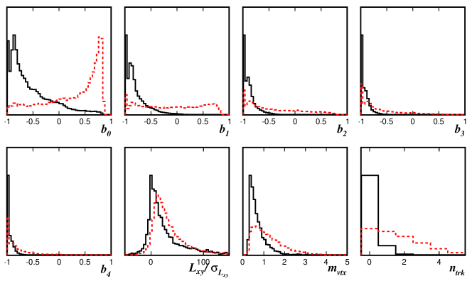
Figure 2: The most relevant inputs used in the neural network for calculating the per-jet $b$ness. The red dashed line is signal and the black solid line is background. $b_{i}$ refers to the $b$ness of the $i$^th track, ordered in $b$ness. The $y$-axis is in arbitrary units.

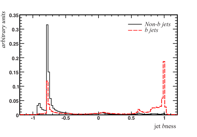
Figure 3: Output of the final neural network, for signal (red dashed line) and background (black solid line). Good separation is seen with the exception of signal (and background) peaking near a jet $b$ness of -0.8. This region is dominated by jets with zero tracks having positive track $b$ness, zero $K_{S}$ candidates found, and no secondary vertex. Indeed, some $b$ jets are indistinguishable from non-$b$ jets. The sharp features of this distribution are a result of the discrete inputs to the NN.

Additionally, because a much higher fraction of $b$ jets than non-$b$ jets contain $K_{S}$ particles, the number of $K_{S}$ candidates found is used as an input to the jet-by-jet NN. Finally, if there is a muon candidate in the jet cone, its likelihood to be a true muon is used as an input. This value is calculated using the soft muon tagger [7] described above. The architecture of the jet-by-jet NN is similar to that of the track-by-track NN, with two hidden layers of 15 and 16 nodes. As in the track NN, to avoid a kinematic bias, the parent jet $E_{T}$ distributions are weighted to be equal and also input into the NN. Distributions of the most important jet-by-jet NN input variables are shown in Figure 2. Distributions of the NN output are shown in Figure 3.

The training for the track NN as well as the jet NN is performed using jets, from a pythia $ZZ$ MC sample, matched to $b$ quarks from $Z\rightarrow b\bar{b}$ events for signal and jets not matched to $b$ quarks for background.

4 Selection for Mistag Rate and Efficiency Determination

$Z+1$ jet Selection
$N_{\text{leptons}}=2$, both electrons or both muons
Leptons have opposite charge
$\Delta z_{0}$ between leptons $<$ 5 cm
Lepton $p_{T}>$ 20 GeV/$c$
75 GeV/$c^{2}<M_{ll}<$ 105 GeV/$c^{2}$
$\mbox{$\not\!\!E_{T}$}<25$ GeV
Reconstructed $p_{T}(Z)>10$ GeV$/c$
$N_{\text{jets}}$($E_{T}>10$ GeV) $=1$
Jet $E_{T}>20$ GeV, $|\eta|<2.0$

$t\bar{t}$ Selection

$N_{\text{leptons}}=1$

Lepton $p_{T}>$ 20 GeV/$c$

$\mbox{$\not\!\!E_{T}$}>20$ GeV

$\not\!\!E_{T}$-significance $>1(3)$ for $\mu(e)$ events

Reconstructed $M_{T}(W)>$ 28 GeV/$c^{2}$

Highest two $b$ness jets’ $E_{T}>$ 20 GeV

$N_{\text{jets}}(E_{T}>15$ GeV) $\geq 4$

Total sum $E_{T}>300$ GeV

Table 1: Summary of event selection requirements for the $Z+1$ jet and $t\bar{t}$ samples. The total sum $E_{T}$ is defined as the sum of the lepton $p_{T}$, $\not\!\!E_{T}$, and $E_{T}$ of all jets with $E_{T}>$ 15 GeV.

In order to use this new $b$ tagger in analyses, we determine the efficiency and false tag (“mistag”) rate as a function of a minimal $b$ness requirement, $e(b)$ and $m(b)$ respectively. We use comparisons between data and Monte Carlo simulation to evaluate these quantities and their uncertainties. Also, we evaluate the efficiency and mistag rate in Monte Carlo ($e_{\text{MC}}(b)$ and $m_{\text{MC}}(b)$, respectively), and determine the necessary scale factor, $s_{e}(b)=e(b)/e_{\text{MC}}(b)$ (with a similar definition for the mistag rate), to correct the simulation.

	Electrons		Muons
$Z+1$ jet selection
Data Events	9512		5575
MC Events	9640$\,\pm\,$	880	5540$\,\pm\,$	490
$t\bar{t}$ Selection
Data Events	507		835
MC Events	542$\,\pm\,$	56	862$\,\pm\,$	85

Table 2: Number of events in data and MC in the $Z+1$ jet selection region, after proper scale factors have been applied. The uncertainties on the MC reflect only the two dominant systematic uncertainties: the uncertainty on the jet energy scale and the uncertainty on the luminosity. Overall, the agreement in number of events is good.

Following the procedure described in A and B, we must choose two independent regions in which to determine the mistag rate and efficiency of the $b$ tagger. To reduce uncertainties, it is best to choose a well-modelled region dominated by falsely tagged jets (where we expect few $b$ jets) and a well-modelled region rich in $b$ jets. For the former, we choose events containing two oppositely charged electrons or muons likely from the decay of a $Z$ boson, plus one jet. For the latter, we choose events containing the decay of a pair of top quarks, where we require exactly one lepton, at least four jets, and a large imbalance in transverse momentum in the event, indicating the likely presence of a neutrino. We expect that the two jets with the highest $b$ness values in this sample will very likely be $b$ jets. The cuts applied for these two selection regions are described in Table 1. We use the $\not\!\!E_{T}$ significance, as defined in [21, 22], to reduce any contribution from multi-jet production where a jet is mis-identified as an electron or muon.

These events are selected by high-$p_{T}$ electron and muon triggers. We use data corresponding to an integrated luminosity of 4.8 fb^-1. We use alpgen [23], interfaced with pythia for parton showering, to model $W$ and $Z$ plus jets samples and pythia to model $t\bar{t}$ and other processes with small contributions. We check the trigger efficiency against a sample of $Z\to e^{+}e^{-}$ or $\mu^{+}\mu^{-}$ events without jets. Table 2 contains a summary of the total number of events.

5 Mistag Rate Determination

Figure 4 shows the jet $b$ness distribution for jets in the $Z$ + 1 jet sample. The sample is dominated by light-flavor jets, but there is a significant contribution of real $b$ jets at higher $b$ness values, coming from $Z+b\bar{b}$ production. This is seen more clearly in Figure 5, where we separate the MC jets based on whether there are generator-level $b$ quarks located within each jet’s cone ($\Delta R=0.4$). Also shown is the $b$-jet purity ($N_{\text{b-jets}}/N_{\text{jets}}$) as a function of lower threshold on jet $b$ness. We see the $b$-jet incidence rate reaches above 60% for the highest $b$ness cuts, and thus we will expect the uncertainties in the mistag rate to be substantially higher there, due to both the small sample of available jets and the high contamination rate combined with the uncertainty on the number of $b$ jets in that smaller sample.

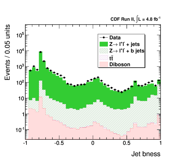
Figure 4: A comparison of the jet $b$ness in data and MC in the $Z+1$ jet selection region. The MC is able to reproduce the main features of the $b$ness distribution in data. We use this distribution to determine the mistag rate for placing a cut on jet $b$ness in data, and use the differences between data and MC to determine corrections to the mistag rate in MC.

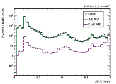
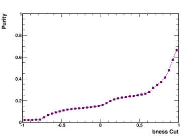
Figure 5: Left: A comparison of the jet $b$ness in data (black points) and MC (green solid line) in the $Z+1$ jet selection region, with the portion of the MC jets matched to $b$ quarks (purple dashed line) shown independently. Right: The $b$-jet purity for a given $b$ness cut, as determined from matched jets in the MC. As we wish to use the $Z+1$ jet sample as a model for mistags, it is necessary to subtract the significant $b$-jet contribution at high $b$ness values.

The mistag rate for jets above a given $b$ness threshold is simply the fraction of non-$b$ jets above that threshold. To obtain this quantity, we use the fraction of jets in data above that threshold ($m_{\text{raw}}(b)$), but must correct this quantity for the expected number of $b$ jets in our $Z+1$ jet sample. We obtain an estimate of this $b$ jet contamination from MC simulation, and obtain the corrected mistag rate, $m(b)$. We show the values of $m(b)$ as well as the relative difference between the mistag rate in data and MC ($s_{m}(b)-1$) in Figure 6.

We can also calculate the uncertainty on the mistag rate given the error on the $b$-tagging efficiency and the uncertainty on the fraction of $b$ jets in our $Z+1$ jet sample. The former is determined through iterative calculations incorporating the $t\bar{t}$ selection, while the latter we take to be 20% [24]. The resulting uncertainties are also shown in Figure 6.

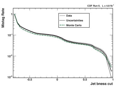
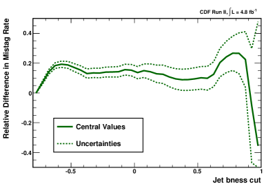
Figure 6: Left: The mistag rate in data (solid black line, dashed lines represent uncertainty) and Monte Carlo (dot-dashed green line) as a function the jet $b$ness. We see our simulation typically under-predicts the mistag rate measured in data, requiring us to consider a correction to apply to the MC. Right: The calculated MC scale factor on the mistag rate (solid line) and its uncertainty (dashed lines) relative to the mistag rate in the Monte Carlo. The value of the scale factors and their uncertainties at the relevant $b$ness cuts in this analysis are summarized in Table 3. We see very large uncertainties on the mistag rate scale factor around the high jet $b$ness cut of 0.85, due to the small number of events and significant heavy-flavor removal that must be done in this region.

6 Tagging Efficiency Determination

We use our $t\bar{t}$ selection, described in Section 4 and Table 1, to calculate the efficiency from a sample of jets with high $b$ purity. As these events have many jets, we order the jets by decreasing $b$ness value. This mirrors the procedure in a related analysis using this $b$ tagger [25] and provides values for the $b$-tagging efficiency while accounting for this sorting procedure. Figure 7 shows the jet $b$ness distributions in data and MC for the two jets with highest $b$ness in each event. The agreement here is very good, and regions of high $b$ness are almost exclusively populated by $t\bar{t}$ events, indicating that our $b$ tagger is properly identifying $b$ jets. We check that the purity of $b$ jets as a function of the cut on the jet $b$ness in these distributions is also high by splitting jets into matched and non-matched categories (Figure 8), as done for the $Z+1$ jet selection described in Section 5. We see that the $b$-jet purity of the $t\bar{t}$ sample is rather high, even for low $b$ness thresholds.

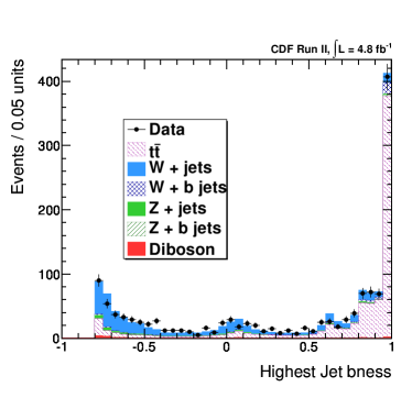
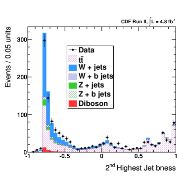
Figure 7: Jet $b$ness of the first (left) and second (right) jet, as ordered by $b$ness, in the $t\bar{t}$ lepton + jets selection region. The simulation reproduces most of the features of the data, and we see much of the $b$-enriched samples clustered towards high $b$ness.

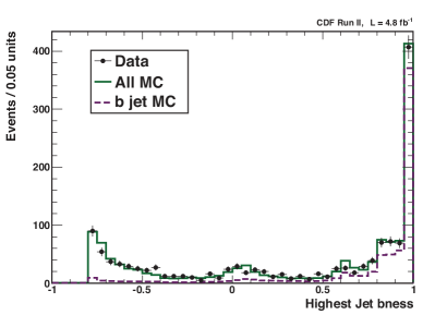
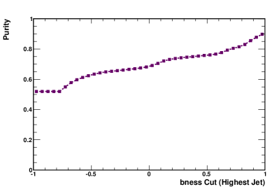
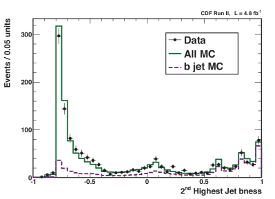
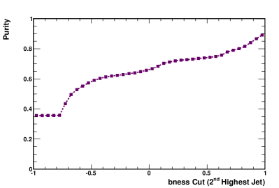
Figure 8: Top Left: A comparison of the highest jet $b$ness in data (black points) and MC (green solid line) in the $t\bar{t}$ lepton + jets sample, with the portion of the MC jets matched to $b$ quarks (purple dashed line) shown independently. Top Right: The $b$-jet purity for a given $b$ness cut on the highest jet $b$ness, as determined from matched jets in the MC. Bottom Left: A comparison of the second highest jet $b$ness in data (black points) and MC (green solid line) in the $t\bar{t}$ lepton + jets selection region, with the portion of the MC jets matched to $b$ quarks (purple dashed line) shown independently. Bottom Right: The $b$-jet purity for a given $b$ness cut on the second highest jet $b$ness, as determined from matched jets in the MC. In these plots, we see a high purity in our chosen sample, which is approximately 55% $t\bar{t}$ events.

We calculate the efficiency of a given $b$ness threshold and its uncertainty in an analogous way to the calculation of the mistag rate, described in detail in B. We show the calculated efficiencies and uncertainties for the highest and 2^nd highest $b$ness jets in Figure 9, and we show the relative difference between the efficiency in data and MC (the quantity $s_{e}(b)-1$) and its uncertainty in Figure 10. The relative differences and uncertainties on the efficiency are on the order of 10% or less, comparable to the SecVtx $b$ tagger scale factors and their uncertainties. Table 3 lists the efficiency and mistag rates in data and MC for a chosen operating point—the highest jet $b$ness $>0.85$, and the 2^nd highest jet $b$ness $>0.0$—along with the relative difference between data and MC, and the error on that difference. This choice of operating points is motivated by the optimization of a cross section measurement that uses the tagger [25]. Figure 11 shows the relationship between the calculated efficiency of identifying $b$ jets with a cut on the jet $b$ness and the rejection power of that cut for non-$b$ jets for the highest and 2^nd highest $b$ness jets in an event.

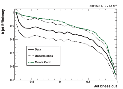
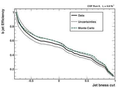
Figure 9: The efficiency of a $b$ness cut in data (solid black line, dashed lines represent uncertainty) and Monte Carlo (dot-dashed green line) as a function of a cut on jet $b$ness for the highest (left) and 2^nd highest (right) $b$ness jets in an event. We see our simulation typically over-predicts the efficiency measured in data, and thus needs to be corrected.

Quantity	$b$ness Cut	Data	MC	% Difference	% Error
Mistag Rate	$0.0$	$0.0819$	$0.0720$	$14\%$	$4.1\%$
	$0.85$	$0.00997$	$0.00869$	$15\%$	$21\%$
Tag Efficiency	$0.0$	$0.622$	$0.684$	$-9.0\%$	$8.7\%$
	$0.85$	$0.652$	$0.687$	$-5.2\%$	$6.2\%$

Table 3: Mistag rates and efficiencies on jet $b$ness cuts determined from comparisons of data and MC in our $Z+1$ jet and $t\bar{t}$ control regions. For the $b$ness cut at 0.85, we consider the highest $b$ness jet, and for the $b$ness cut at 0.0, we consider the 2^nd highest $b$ness jet in our $t\bar{t}$ sample.

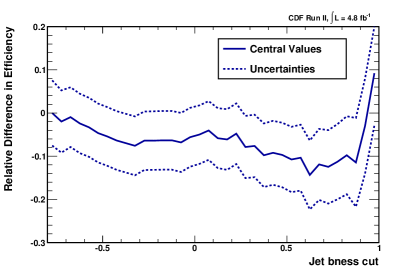
Figure 10: The difference in efficiency between data and Monte Carlo (center solid line) and its uncertainty (dashed lines) relative to the efficiency in the Monte Carlo as a function of the cut on jet $b$ness for the highest (left) and 2^nd highest (right) $b$ness jets in an event. The value of the scale factors and their uncertainties at the relevant $b$ness cuts in this analysis are summarized in Table 3.

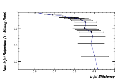
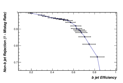
Figure 11: Plots of the non-$b$-jet rejection versus the $b$-jet efficiency for a range of a cuts on jet $b$ness for the highest (left) and 2^nd highest (right) $b$ness jets in an event.

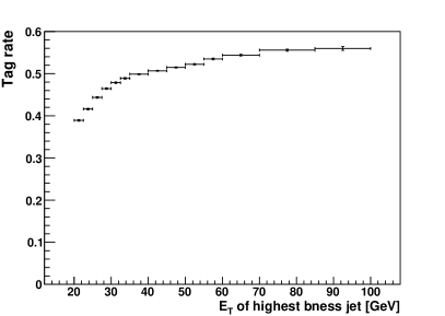
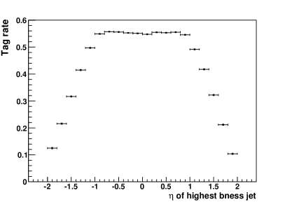
Figure 12: Tag performance for the jet with the highest $b$ness score as a function of transverse momentum (left) and $\eta$ (right) for a $b$ness requirement $b>0.85$, derived from simulated data. The tagging efficiency ranges from 38% at low transverse momentum to more than 50% at higher momentum. The efficiency is flat in the central region ($|\eta|<1.0$) and drops outside the acceptance of the central part of the tracking system.

We estimate the performance of the tagger as a function of the jets’ transverse momenta and pseudorapidity in simulated data of di-jet events, where the jets are $b$ jets. We select the jet with the highest $b$ness score and calculate the efficiency for $b$ness $>0.85$. These efficiencies are shown in Figure 12. The tagging efficiency ranges from 38% at low transverse momentum to more than 50% at higher momentum. The efficiency is flat in the central region ($|\eta|<1.0$) and drops outside the acceptance of the central part of the tracking system.

While generic comparisons between taggers are difficult, we compare our tagger to the most commonly used $b$ tagger in CDF, the SecVtx tagger. The efficiency and mistag rates of our tagger compare favorably to the SecVtx tagger. We compare the two taggers using simulated events, looking at the two highest $b$ness jets in the MC of our $t\bar{t}$ selection, and look at require $b>0.85$ for our tagger. The “tight” SecVtx tagger operating point on this sample of jets has an efficiency of $0.59$ and a mistag rate of $0.052$, while the “loose” operating point has an efficiency of $0.68$ with a mistag rate of $0.088$. For the highest $b$ness jet cut at $>0.85$, we have a efficiency near the loose-tag efficiency ($0.69$), but a lower mistag rate ($0.009$) than the tight SecVtx tag; for the 2^nd highest $b$ness jet cut at $>0.0$, we have a similarly high efficiency ($0.68$) while allowing a mistag rate similar to the loose SecVtx tag ($0.082$).

7 Conclusion

We have described a neural network based $b$ tagger in current use at the Fermilab Tevatron’s CDF experiment. By examining all the tracks associated with jets, this tagger has a larger acceptance than previous neural network based taggers at CDF. Furthermore, the tagger is calibrated using data from $Z$ boson decays and events containing top quark pair production—a novel method which yields small systematic uncertainties on the tagging efficiency and mistag rate. Finally, the utility of this tagger has been demonstrated in a measurement of the $ZZ$ and $WZ$ production cross sections [25].

Appendix A Evaluation of Mistag Rate and Efficiency

For any given selection of data, we can calculate the mistag rate (where all non-$b$ jets are considered mistags) if we know the number $N_{B}$ of $b$ jets, the number $N_{B}(b)$ of $b$ jets above the threshold $b$ness, the total number $N$ of jets, and the total number $N(b)$ of jets above the $b$ness cut threshold:

$$m(b)=\frac{N(b)-N_{B}(b)}{N-N_{B}}.$$ (1)

We may use MC to determine the fraction $f_{B}$ of jets that are $b$ jets, and the efficiency $e_{\text{MC}}(b)$ for these jets to pass the $b$ness cut. This efficiency may need to be modified by a scale factor $s_{e}(b)=e(b)/e_{\text{MC}}(b)$ if it is different from the true efficiency evaluated in data. Thus,

$$N_{B}=f_{B}N\text{~{}~{}and~{}~{}}N_{B}(b)=s_{e}(b)e_{\text{MC}}(b)f_{B}N.$$ (2)

Also, if we define a mistag rate that has not been corrected for the possible presence of $b$ jets in the same sample, $m_{\text{raw}}(b)=N(b)/N$, then we may write equation 1 in the following way:

$$m(b) =\frac{m_{\text{raw}}(b)N-s_{e}(b)e_{\text{MC}}(b)f_{B}N}{N-f_{B}N}$$

$$=\frac{m_{\text{raw}}(b)-s_{e}(b)e_{\text{MC}}(b)f_{B}}{1-f_{B}}.$$ (3)

We can write an analogous expression for the efficiency of $b$ jets passing a given $b$ness cut:

$$e(b)=\frac{e_{\text{raw}}(b)-s_{m}(b)m_{\text{MC}}(b)f_{L}}{1-f_{L}}$$ (4)

where $e_{\text{raw}}(b)$ is a “raw” efficiency uncorrected for the presence of non-$b$ jets in a sample, $m_{\text{MC}}(b)$ is the mistag rate as measured in MC, corrected to match data by a scale factor $s_{m}(b)$, and $f_{L}$ is the fraction of light-flavor (here defined as non-$b$) jets in the chosen sample.

Note that the determination of the mistag rate depends on the calculated value of the efficiency (through the scale factor term $s_{e}(b)$), and that in turn the determination of the efficiency depends on the mistag rate (again through the scale factor $s_{m}(b)$). Similarly, the uncertainties on these quantities (see below) depend on each other in a non-linear fashion. Thus, we use an iterative procedure to solve for the mistag rate, efficiency, and their uncertainties. We calculate the mistag rate first using a value of $s_{e}(b)=1$, and find that the values of $e(b)$ and $m(b)$ converge (and their uncertainties) very quickly.

The uncertainties on these quantities may also be calculated from the expressions above. For the mistag rate,

$$\sigma_{m}^{2}(b) =\frac{m_{\text{raw}}(b)(1-m_{\text{raw}}(b))}{N(1-f_{B})^{2}}$$

$$+\left(\frac{\sigma_{e}(b)f_{B}}{1-f_{B}}\right)^{2}$$

$$+\left(\frac{\sigma_{f_{B}}[s_{e}(b)e(b)-m(b)]}{1-f_{B}}\right)^{2}.$$ (5)

The first term is a binomial uncertainty on the raw mistag rate of the sample, and is the term related to the statistical uncertainty of the sample used to determine the mistag rate. The second term comes from the uncertainty on the measured value of $e(b)$, which can be calculated using a similar expression, and is done so iteratively, as $\sigma_{m}(b)$ and $\sigma_{e}(b)$ depend on each other. The final term is due to the uncertainty on $f_{B}$, which will depend on the choice of MC and the region in which MC and data are compared. A similar expression determines $\sigma_{e}(b)$.

Appendix B Tagging Efficiency Determination

Similar to our calculation of the mistag rate, we calculate the efficiency observed in data using equation 4. Both $e_{\text{raw}}(b)$ and $s_{m}(b)m_{\text{MC}}(b)=m(b)$ can be calculated easily by counting events above a given $b$ness threshold in the data and MC respectively. Because of the different competing processes in our $t\bar{t}$ sample (there is a significant contribution from $W$ + light flavor jets and $W$ + $b\bar{b}$ processes), it is best to break $f_{L}$ into these most significant subsamples:

$$f_{L}=\frac{f_{L}^{Wjj}N_{Wjj}+f_{L}^{Wb\bar{b}}N_{Wb\bar{b}}+f_{L}^{t\bar{t}}N_{t\bar{t}}}{N_{Wjj}+N_{Wb\bar{b}}+N_{t\bar{t}}}$$ (6)

where $N_{X}$ is the number of events predicted by MC in subsample $X$, and $f_{L}^{X}$ is the fraction of non-$b$ jets in subsample $X$. We assume that the MC correctly reproduces the values of $f_{L}^{X}$. To determine $s_{e}(b)=e(b)/e_{\text{MC}}(b)$, we write down a similar expression for the efficiency in MC using the efficiency of each subsample in MC:

$$e_{\text{MC}}(b)=\frac{1}{N_{Wjj}+N_{Wb\bar{b}}+N_{t\bar{t}}}\sum_{X}e_{X}(b)f_{B}^{X}N_{X}$$ (7)

where, as before, $N_{X}$ is the number of events predicted by Monte Carlo in subsample $X$, $f_{B}^{X}$ is the total fraction of $b$ jets in subsample $X$, and $e_{X}$ is the efficiency of $b$ jets passing a particular $b$ness cut in subsample $X$. We assume, again, that the Monte Carlo correctly reproduces the values of $f_{B}^{X}$.

Given Equations 6 and 7, we modify our equation for determining the uncertainty in the calculated efficiency. We obtain the uncertainty by calculating the uncertainty of the quantity $(e(b)-e_{\text{MC}}(b))$, and find

$$\sigma_{e}^{2}(b) =\frac{1}{(1-f_{L})^{2}}\left(\frac{e_{\text{raw}}(1-e_{\text{raw}})}{N_{D}}+(\sigma_{m}f_{L})^{2}\right)$$

$$+\sum_{X}\frac{\sigma_{X}^{2}}{\left[N_{\text{MC}}(1-f_{L})\right]^{2}}\times$$

$$\left[(e+s_{m}m)(f_{L}-f_{L}^{X})\right.\left.+f_{B}^{X}(e_{\text{MC}}-e_{X})\right]^{2}$$ (8)

where the latter term represents a sum over each of the MC subsamples. $N_{\text{MC}}$ and $N_{B}$ are the total number of events and events with $b$ jets in the MC, and $\sigma_{X}$ is the uncertainty assigned to the number of events in each MC subsample. Because we compare only the normalizations of data and MC in our determination of efficiency (and mistag rate) scale factors, the uncertainty on the number of events in each MC subsample need only reflect the relative uncertainty on the fraction of events each subsample contributes to the whole. We assign $\sigma_{Wb\bar{b}}=20\%$, and $\sigma_{Wjj}=8.72\%$ and $\sigma_{t\bar{t}}=6.78\%$ based on a fit to the distribution of the sum of the highest two $b$ness jets in $t\bar{t}$ events.

References

- Abe et al. [1994] F. Abe, et al., Phys. Rev. D 50 (1994) 2966.
- Abazov et al. [2010] V. M. Abazov, et al., Nucl. Instrum. Methods A 620 (2010) 490.
- CMS Collaboration [2011] CMS Collaboration, CMS Physics Analysis Summary CMS-PAS-BTV-11-001 (2011).
- ATLAS Collaboration [2011] ATLAS Collaboration, ATLAS CONF Note ATLAS-CONF-2011-102 (2011).
- Acosta et al. [2005] D. Acosta, et al., Phys. Rev. D 71 (2005) 052003.
- Abulencia et al. [2006] A. Abulencia, et al., Phys. Rev. D 74 (2006) 072006.
- Acosta et al. [2005] D. Acosta, et al., Phys. Rev. D 72 (2005) 032002.
- Richter [2007] S. Richter, FERMILAB-THESIS-2007-35 (2007).
- Aaltonen et al. [2010] T. Aaltonen, et al., Phys. Rev. D 82 (2010) 112005.
- Ferrazza [2006] C. Ferrazza, Identificazione di quark pesanti in getti adronici in interazioni con il rivelatore CDF al Tevatron, Master’s thesis, Università “La Sapienza” Roma, 2006.
- Mastrandrea [2008] P. Mastrandrea, FERMILAB-THESIS-2008-63 (2008).
- Abulencia et al. [2007] A. Abulencia, et al., J. Phys. G 34 (2007) 2457.
- Affolder et al. [2004] T. Affolder, et al., Nucl. Instrum. Methods A 526 (2004) 249.
- Abe et al. [1992] F. Abe, et al., Phys. Rev. D 45 (1992) 1448.
- Bhatti et al. [2006] A. Bhatti, et al., Nucl. Instrum. Methods A 566 (2006) 375.
- Brun et al. [1978] R. Brun, et al., geant3 manual, 1978. CERN Report CERN-DD-78-2-REV (unpublished).
- Campbell and Ellis [1999] J. M. Campbell, R. K. Ellis, Phys. Rev. D 60 (1999) 113006.
- Pumplin et al. [2002] J. Pumplin, et al., J. High Energy Phys. 0207 (2002) 012.
- Sjöstrand et al. [2006] T. Sjöstrand, et al., J. High Energy Phys. 05 (2006) 026.
- Hoecker et al. [2007] A. Hoecker, P. Speckmayer, J. Stelzer, J. Therhaag, E. von Toerne, H. Voss, PoS ACAT (2007) 040.
- Aaltonen et al. [2009] T. Aaltonen, et al., Phys. Rev. Lett. 103 (2009) 091803.
- Goncharov et al. [2006] M. Goncharov, et al., Nucl. Instrum. Methods A 565 (2006) 543.
- Mangano et al. [2003] M. L. Mangano, et al., J. High Energy Phys. 07 (2003) 001.
- Aaltonen et al. [2009] T. Aaltonen, et al., Phys. Rev. D 79 (2009) 052008.
- Aaltonen et al. [2011] T. Aaltonen, et al., arXiv:1108.2060 (2011).