Chiral Symmetry Breaking and Confinement Beyond Rainbow-Ladder Truncation

Abstract

A non-perturbative construction of the 3-point fermion-boson vertex which obeys its Ward-Takahashi or Slavnov-Taylor identity, ensures the massless fermion and boson propagators transform according to their local gauge covariance relations, reproduces perturbation theory in the weak coupling regime and provides a gauge independent description for dynamical chiral symmetry breaking (DCSB) and confinement has been a long-standing goal in physically relevant gauge theories such as quantum electrodynamics (QED) and quantum chromodynamics (QCD). In this paper, we demonstrate that the same simple and practical form of the vertex can achieve these objectives not only in 4-dimensional quenched QED (qQED4) but also in its 3-dimensional counterpart (qQED3). Employing this convenient form of the vertex ansatz into the Schwinger-Dyson equation (SDE) for the fermion propagator, we observe that it renders the critical coupling in qQED4 markedly gauge independent in contrast with the bare vertex and improves on the well-known Curtis-Pennington construction. Furthermore, our proposal yields gauge independent order parameters for confinement and DCSB in qQED3.

I Introduction

Schwinger-Dyson equations (SDEs) are the fundamental field equations of any quantum field theory. As their derivation requires no recourse to the value of the interaction strength, they are ideally suited for perturbative as well as non-perturbative realms of basic interactions. In particular, they provide an excellent framework for a unified description of those field theories for which the evolution of the beta function encodes diametrically opposed dynamics simultaneously: asymptotic freedom in the ultraviolet and dynamical chiral symmetry breaking (DCSB) and confinement in the infrared. Consequently, continuum studies of the long-range behavior of quantum chromodynamics (QCD), where effective degrees of freedom are mesons and baryons, have been vastly carried out through SDEs. It also allows to extract predictions for the transition region where perturabtive and non perturbative facets of QCD coexist as well as for the short distance physics where the fundamental degrees of freedom are quarks and gluons.

Some original works on DCSB in QCD through SDEs can be dated back to Higa:1984 ; Miransky:1985 . The most natural and practical truncation of the infinite set of these equations is carried out at the level of the fermion-boson vertex, see for example Roberts-review:1994 ; Fischer:2006 ; Bashir-Raya-Review:2006 ; Fischer:1994 for detailed discussions on the subject. The rainbow-ladder truncation is sufficient to reproduce a large body of existing experimental data on pseudoscalar and vector mesons such as their masses, charge radii, decay constants and scattering lengths as well as their form factors and the valence quark distribution functions Roberts-Maris:1997 ; Tandy-Maris:2000 ; Tandy-Maris:2002 ; Ji-Maris:2001 ; Tandy-Maris:1999 ; Tandy-Maris:2003 ; Maris:2002 ; Cotanch-Maris:2002 ; Bashir-Guerrero-1:2010 ; Bashir-Guerrero-2:2010 ; Tandy-Nguyen:2011 .

However, a fully dressed 3-point fermion-boson vertex is required to extend the domain of success provided by the SDEs within their unified description of hadronic physics. For example, although the $\pi$- and $\rho$-mesons are described rightfully by the rainbow-ladder truncation, their parity partners, namely, the $\sigma$- and the $a_{1}$-mesons are not. The underlying reason has been recently discovered to be linked with the fact that DCSB generates a large dressed-quark anomalous chromomagnetic moment. As a result, spin-orbit splitting between ground-state mesons is dramatically enhanced. This is the mechanism responsible for a magnified splitting between parity partners. The essentially nonperturbative corrections to the rainbow-ladder truncation largely cancel in the pseudoscalar and vector channels but add constructively in the scalar and axial-vector channels, providing a clear signal to go beyond the rainbow-ladder for these mesons, Roberts-Chang:2009 ; Roberts-Chang:2011 .

On the theoretical side, research efforts spanning a couple of decades on various gauge field theories such as scalar QED Bashir-Concha:2007 ; Bashir-Concha:2009 ; Bashir-Concha:2010 , spinor QED Ball:80 ; Curtis:90 ; Bashir:94 ; Bashir:96 ; Kizilersu:95 ; Kizilersu:09 ; Bashir-Guerrero:2011 , field theories in different space-time dimensions Burden:93 ; Dong:1994 ; Bashir:98 ; Bashir:01 ; Bashir:04 and QCD Skullerud:2003 ; Skullerud:2007 ; Aguilar:2010 have revealed that gauge invariance Burden:93 ; Bashir:94 ; Bashir:96 ; Bashir:thesis ; Bashir:02 , gauge covariance (which is a statement of multiplicative renormalizability of the 2-point function in 4 dimensions) Curtis:90 ; Bashir-Kizilersu:1998 and perturbation theory Ball:80 ; Kizilersu:95 ; Bashir:99 ; Davydychev:2000 ; Bashir:01 ; Bashir-Concha:2007 impose severe constraints on the fermion-boson interaction. The gauge technique of Delbourgo and Salam Salam:1964 ; Delbourgo-1:1977 ; Delbourgo-2:1977 ; Delbourgo:1979 , introduced decades earlier, was in fact developed to address some of these constraints, namely the ones which stem from gauge invariance. This technique culminated in formal results for the fermion-boson vertex expressed in terms of spectral functions Delbourgo:1981 ; Delbourgo:1987 . However, this approach is cumbersome in practical calculations of the fermion propagator Parker:1984 ; Delbourgo:1984 .

All the studies to-date imply that the 3-point vertex projected onto the propagator equations is largely determined by the behavior of the fermion propagator itself and not by the knowledge of the higher-point functions. There exist numerous ans$\ddot{a}$tze for the transverse part of the vertex (which remains unfixed by the constraints of gauge invariance) involving different forms of the functional dependence on the 2-point functions, depending upon the case at hand. In this article, we provide first steps towards a unified approach for this truncation, applicable to different problems. We employ a simple and practical form for the full fermion-boson vertex which respects its Ward-Takahashi identity, yields a fermion propagator which respects its gauge covariance properties, has the correct charge conjugation properties and also reproduces its asymptotic perturbative limit both in QED3 and QED4. Moreover, it not only renders the critical coupling in qQED4 markedly gauge independent Bashir:thesis in contrast with the bare vertex and improves on the Curtis-Pennington vertex Curtis:90 but also yields gauge independent order parameters for confinement and DCSB in qQED3.

This paper is organized as follows: In Sect. II we decompose the full fermion-boson vertex into its longitudinal and transverse parts, invoking Ward-Takahashi identity (WTI) for QED. Employing a simple ansatz for the transverse vertex based upon the key features of qQED4 reduces the gauge dependence of the critical coupling Bashir:thesis in comparison with even one of the most sophisticated vertices constructed to date, namely, Curtis-Pennington vertex Curtis:90 . In Sect. III, we use the same functional form of the ansatz to study DCSB and confinement in qQED3. The corresponding order parameters are again found to be gauge independent. We provide a convincing comparison with the results obtained by employing the Curtis-Pennington vertex Curtis:90 as well as the Burden-Roberts vertex Burden:1991 . Conclusions and plans for further work are presented in Sect. IV.

II Transverse Vertex: DCSB in QED4

The SDE for the fermion propagator in QED is expressed as

$$S_{F}^{-1}(p) = S_{F}^{(0)\,-1}(p)$$ (1)

$$- 4\pi i\alpha\int\frac{d^{d}k}{(2\pi)^{d}}\ \gamma^{\mu}S_{F}(k)\Gamma^{\nu}(k,p)\Delta_{\mu\nu}(q)\;,$$

in arbitrary space-time dimensions $d$. Here $\alpha$ is the electromagnetic coupling (dimensional for $d\neq 4$), $S_{F}(p)$ is the fermion propagator, $S_{F}^{(0)}(p)$ is its bare counterpart, $\Delta_{\mu\nu}(q)$ (with $q=k-p$) is the gauge boson propagator and $\Gamma^{\nu}(k,p)$ is the fermion-boson vertex. We can write the fermion propagator in the following equivalent forms :

$$S_{F}(p) = \sigma_{V}(p^{2}){\not\!p}+\sigma_{S}(p^{2})$$ (2)

$$= \frac{F(p)}{{\not\!p}-M(p)}\ =\ \frac{F(p)({\not\!p}+M(p))}{p^{2}-M^{2}(p)}\;,$$

$F(p)$ being the fermion wavefunction renormalization and $M(p)$, the mass function. Correspondingly, we can write $S_{F}^{(0)}(p)=1/({\not\!p}-m)$, where $m$ denotes the bare fermion mass. In this article, we work in the chiral limit by setting $m=0$. In quenched QED, the full gauge boson propagator receives no radiative corrections, i.e.,

$$\Delta_{\mu\nu}(q)=\Delta_{\mu\nu}^{(0)}(q)=-\frac{1}{q^{2}}\left[g_{\mu\nu}+(\xi-1)\frac{q_{\mu}q_{\nu}}{q^{2}}\right]\;,$$

where $\xi$ is the usual covariant gauge parameter such that $\xi=0$ corresponding to the Landau gauge. To be able to solve the gap equation (1), we must know the explicit form of the fermion-boson interaction $\Gamma^{\mu}(k,p)$. It is related to the fermion propagator through the WTI :

$$q_{\mu}\Gamma^{\mu}(k,p)=S_{F}^{-1}(k)-S_{F}^{-1}(p)\;.$$ (3)

This identity motivates a natural decomposition of the vertex into its longitudinal and transverse parts,

$$\Gamma^{\mu}(k,p)=\Gamma^{\mu}_{L}(k,p)+\Gamma^{\mu}_{T}(k,p)\;,$$ (4)

where the transverse vertex is defined to be such that $q_{\mu}\Gamma^{\mu}_{T}(k,p)=0$ and $\Gamma^{\mu}(p,p)=0$. Following Ball and Chiu, we choose the longitudinal part of the vertex to be Ball:80 ,

$$\Gamma^{\mu}_{L}(k,p) = \frac{\gamma^{\mu}}{2}\left[\frac{1}{F(k)}+\frac{1}{F(p)}\right]$$ (5)

$$+ \frac{1}{2}\,\frac{({\not\!k}+{\not\!p})(k+p)^{\mu}}{(k^{2}-p^{2})}\left[\frac{1}{F(k)}-\frac{1}{F(p)}\right]$$

$$- \frac{(k+p)^{\mu}}{(k^{2}-p^{2})}\left[\frac{M(k)}{F(k)}-\frac{M(p)}{F(p)}\right]\;,$$

$$\equiv a(k^{2},p^{2})\gamma^{\mu}+b(k^{2},p^{2})({\not\!k}+{\not\!p})(k+p)^{\mu}$$

$$+ c(k^{2},p^{2}){(k+p)^{\mu}}\;.$$

The transverse part is conveniently expressed as Ball:80

$$\Gamma^{\mu}_{T}(k,p)=\sum_{i=1}^{8}\tau_{i}(k^{2},p^{2},q^{2})T^{\mu}_{i}(k,p)\;,$$ (6)

where the basis vectors are defined to be :

$$T^{\mu}_{1} = p^{\mu}(k\cdot q)-k^{\mu}(p\cdot q)$$

$$T^{\mu}_{2} = \left[p^{\mu}(k\cdot q)-k^{\mu}(p\cdot q)\right]({\not\!k}+{\not\!p})$$

$$T^{\mu}_{3} = q^{2}\gamma^{\mu}-q^{\mu}{\not\!q}$$

$$T^{\mu}_{4} = \left[p^{\mu}(k\cdot q)-k^{\mu}(p\cdot q)\right]k^{\lambda}p^{\nu}{\sigma_{\lambda\nu}}$$

$$T^{\mu}_{5} = q_{\nu}{\sigma^{\nu\mu}}$$

$$T^{\mu}_{6} = \gamma^{\mu}(p^{2}-k^{2})+(p+k)^{\mu}{\not\!q}$$

$$T^{\mu}_{7} = \frac{1}{2}(p^{2}-k^{2})\left[\gamma^{\mu}({\not\!p}+{\not\!k})-p^{\mu}-k^{\mu}\right]$$

$$+\left(k+p\right)^{\mu}k^{\lambda}p^{\nu}\sigma_{\lambda\nu}$$

$$T^{\mu}_{8} = -\gamma^{\mu}k^{\nu}p^{\lambda}{\sigma_{\nu\lambda}}+k^{\mu}{\not\!p}-p^{\mu}{\not\!k}$$ (7)

with $\sigma_{\mu\nu}=[\gamma_{\mu},\gamma_{\nu}]/2.$ This special choice of the transverse vertex was put forward by Ball and Chiu Ball:80 . They carried out a one loop calculation of the fermion-boson vertex in the Feynman gauge. They found the transverse vertex to be independent of any kinematic singularities when $k^{2}\rightarrow p^{2}$. The above choice of the transverse basis guarantees that the coefficient of every individual basis vector in the Feynman gauge is also free of these singularities . It was later pointed out in Kizilersu:95 that this attractive feature of the basis no longer prevails beyond the Feynman gauge even at the one loop level. However, one can re-arrange the basis vectors to restore this quality.

In articles Bashir:94 ; Bashir:96 , Bashir and Pennington proposed a family of transverse vertices, which, by construction, render the critical value of electromagnetic coupling, above which chiral symmetry is restored, completely gauge independent. However, the form of the resulting vertex involves intricate dependence on the elements which define the fermion propagator. Hence its implementation away from the critical coupling is not computationally economical. The same is true for the more recent and complete construction provided in Kizilersu:09 which involves the photon momentum $q$ in its construction. However, it is clear from the perturbative calculation in Davydychev:2000 that an explicit $q^{2}$ dependence occurs in every term of each of the $\tau_{i}$. Therefore, we should keep in mind that whenever we neglect the $q^{2}$ dependence, we are only referring to an effective vertex. However, there exists an exact relation between the real $\tau_{i}(k^{2},p^{2},q^{2})$ and the effective $\tau_{i}^{\rm eff}(k^{2},p^{2})$ as spelled out in Bashir:98 , and utilized in Kizilersu:09 . Before we outline this relation, we also demand that a chirally-symmetric solution should be possible when the bare mass is zero, just as in perturbation theory. This is most easily accomplished if only those transverse vectors with odd numbers of gamma matrices contribute to the transverse vertex. Then the sum in Eq. (6) involves just $i=2,3,6$ and $8$. In the chirally symmetric limit, Eq. (1) yields :

$$\frac{1}{F(p^{2})} = 1-\frac{e^{2}}{p^{2}}\int\frac{d^{d}k}{(2\pi)^{d}}\frac{F(k^{2})}{k^{2}q^{2}}$$ (8)

$$\Big{\{}a(k^{2},p^{2})\frac{1}{q^{2}}[(1-d)q^{2}(k\cdot p)-2\Delta^{2}]$$

$$+ b(k^{2},p^{2})\frac{1}{q^{2}}[-2\Delta^{2}(k^{2}+p^{2})]$$

$$- \frac{\xi}{F(p^{2})}\frac{p^{2}}{q^{2}}(k^{2}-k\cdot p)$$

$$+ \tau_{2}(k^{2},p^{2},q^{2})[-\Delta^{2}(k^{2}+p^{2})]$$

$$+ \tau_{3}(k^{2},p^{2},q^{2})[(d-1)q^{2}(k\cdot p)+2\Delta^{2}]$$

$$- \tau_{6}(k^{2},p^{2},q^{2})[(d-1)(k^{2}-p^{2})k\cdot p]$$

$$- \tau_{8}(k^{2},p^{2},q^{2})[\Delta^{2}(d-2)]\Big{\}}\;,$$

where $\Delta^{2}=(k\cdot p)^{2}-k^{2}p^{2}$. At this stage, it appears impossible to proceed any further without demanding that the $\tau_{i}$ be independent of the angle between the fermion momentum vectors $k$ and $p$, i.e., independent of $q^{2}$. This assumption allows us to carry out the angular integration. In order to distinguish the transverse components which are assumed to be independent of $q^{2}$ from the real ones which explicitly depend on $q^{2}$, we can denote the former by $\tau_{i}^{eff}$. The equation which then emerges after the angular integration can be compared to Eq. (8), giving rise to the following exact relation in arbitrary dimensions :

$$\tau_{2}^{eff} = \int d\psi\frac{{\rm sin}^{d-2}\psi}{q^{2}}\tau_{2}[-\Delta^{2}]$$

$$\tau_{3}^{eff} = \int d\psi\frac{{\rm sin}^{d-2}\psi}{q^{2}}\tau_{3}[2\Delta^{2}+(d-1)(k\cdot p)q^{2}]$$

$$\tau_{6}^{eff} = \int d\psi\frac{{\rm sin}^{d-2}\psi}{q^{2}}\tau_{6}[k\cdot p]$$

$$\tau_{8}^{eff} = \int d\psi\frac{{\rm sin}^{d-2}\psi}{q^{2}}\tau_{8}[\Delta^{2}]\;.$$ (9)

For the desired convenience, we have used the compact notation $\tau_{i}^{eff}(k^{2},p^{2})=\tau_{i}^{eff}$ and $\tau_{i}(k^{2},p^{2},q^{2})=\tau_{i}$. This relationship, of course, depends upon the space-time dimension $d$. It allows us to propose an ansatz for an effective but simple $q^{2}-$independent vertex which fulfills the general requirements that any transverse vertex must satisfy :

$$\Gamma^{\mu}_{T}(k,p) = \sum_{i=2,3,6,8}\tau_{i}^{\rm eff}(k^{2},p^{2})T^{\mu}_{i}(k,p)\;,$$ (10)

where

$$\tau_{2}^{\rm eff}(k^{2},p^{2}) = \frac{{\mathbf{a}}_{2}^{d}}{(k^{4}-p^{4})}\;\left[\frac{1}{F(k)}-\frac{1}{F(p)}\right]\;,$$ (11)

$$\tau_{3}^{\rm eff}(k^{2},p^{2}) = \frac{{\mathbf{a}}_{3}^{d}}{(k^{2}-p^{2})}\;\left[\frac{1}{F(k)}-\frac{1}{F(p)}\right]\;,$$ (12)

$$\tau_{6}^{\rm eff}(k^{2},p^{2}) = \frac{{\mathbf{a}}_{6}^{d}(k^{2}+p^{2})}{(k^{2}-p^{2})^{2}}\;\left[\frac{1}{F(k)}-\frac{1}{F(p)}\right]\;,$$ (13)

$$\tau_{8}^{\rm eff}(k^{2},p^{2}) = \frac{{\mathbf{a}}_{8}^{d}}{(k^{2}-p^{2})}\;\left[\frac{1}{F(k)}-\frac{1}{F(p)}\right]\;.$$ (14)

This construction draws on a direct comparison with the structural dependence of the longitudinal vertex on the elements which make up the fermion propagator. Special care has been taken such that the perturbative limit of the transverse vertex conforms with its one loop expansion in the asymptotic limit of $k^{2}>>p^{2}$. Moreover, it is required to transform correctly under the charge conjugation and parity operations.

Due to the dimension-dependence of the exact connection of these effective $\tau_{i}(k^{2},p^{2})$ with the real $\tau_{i}(k^{2},p^{2},q^{2})$, the least we expect is that the coefficients ${\mathbf{a}}_{i}^{d}$ would depend on the space-time dimensions, justifying the use of the symbol. In 4 space-time dimensions, parameters ${\mathbf{a}}_{i}$ are constrained by the requirement of multiplicative renormalizability of the massless fermion propagator in the following manner :

$$1+{\mathbf{a}}_{2}^{4}+2{\mathbf{a}}_{3}^{4}+2{\mathbf{a}}_{8}^{4}-2{\mathbf{a}}_{6}^{4} = 0\;.$$ (15)

Additionally, one loop perturbative calculation of the transverse fermion-boson vertex in an arbitrary covariant gauge reveals that

$$\Gamma^{\mu}_{T}(k,p) \stackrel{{\scriptstyle k^{2}>>p^{2}}}{{=}} -\frac{\alpha\xi}{8\pi}\;{\rm ln}\frac{k^{2}}{p^{2}}\;\left[\gamma^{\mu}-\frac{k^{\mu}{\not\!k}}{k^{2}}\right]$$ (16)

This perturbative condition imposes the following constraint on the ${\mathbf{a}}_{i}$ :

$${\mathbf{a}}_{3}^{4}+{\mathbf{a}}_{6}^{4} = \frac{1}{2}\;.$$ (17)

It is worth noting that the choice ${\mathbf{a}}_{6}^{4}=1/2$, ${\mathbf{a}}_{3}^{4}=0$ corresponds to the Curtis-Pennington vertex Curtis:90 . Enjoying a broader choice of available parameters, which also includes ${\mathbf{a}}_{2}^{4}$ and ${\mathbf{a}}_{8}^{4}$ (taken to be zero in Curtis:90 ), we expect to construct an improved truncation of the SDEs. It is easy to verify that with the choice of the transverse vertex defined by

$${\mathbf{a}}_{6}^{4}=-\frac{1}{2}\qquad\mbox{and}\qquad{\mathbf{a}}_{2}^{4}=\frac{11}{4}\;$$ (18)

and then inserted into the gap equation (1), that the critical value of the coupling for masses to be dynamically generated, i.e., $\alpha_{c}$, turns out to be considerably more gauge independent for a broad range of values of the covariant gauge parameter $\xi$ not only as compared to the bare vertex but also to the Curtis-Pennington vertex by a fair amount of margin Curtis:90 ; Bashir:thesis . This has been depicted in Fig. (1). We now turn our attention to QED3.

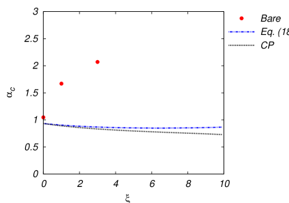
Figure 1: Critical coupling in QED4 as a function of the gauge parameter. The choice of the vertex suggested in Eq. (18) renders the critical coupling in qQED4 markedly gauge independent in contrast with the bare vertex and also improves on the Curtis-Pennington (CP) vertex.

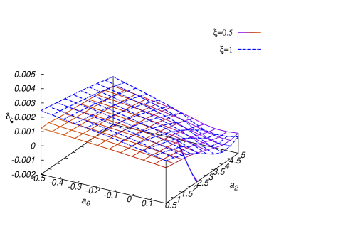
Figure 2: Gauge difference of the condensate as compared to the Landau gauge, Eq. (21), over the ${\mathbf{a}}_{2}/{\mathbf{a}}_{6}$-plane. Solid surface corresponds to $\xi=0.05$, dot-dashed surface to $\xi=1$ and the dotted surface to $\xi=1.5$. Contour of gauge independence of the condensate is along the straight line given by Eq. (22). The scale of the height of the surfaces is set by the value $e^{2}=1$.

III Gauge Independence in QED3

Quantum electrodynamics in (2+1)-dimensions, i.e. QED3, is an interesting theory. It exhibits confinement and DCSB. Therefore, for the last three decades, it has served as a toy model for QCD to deepen our understanding of these fascinating yet complicated phenomena through the efficient tools of SDEs as well as lattice Pisarski:1984 ; Appelquist:1985 ; Pennington:1991 ; Pennington:1992 ; Strouthos:2002 ; Strouthos:2004 ; Bashir-Roberts:2008 ; Zong:2008 ; Fischer:2009 ; Zong:2010 ; Strouthos:2010 ; Swanson:2011 ; Fischer:2011 . It is also of interest in condensed matter physics as an effective field theory for high-temperature superconductors Franz:01 ; Franz:02 ; Tesanovic:02 ; Herbut:02 ; Thomas:07 and graphene Novoselov:05 ; Gusynin:07 ; Riazuddin:2011 .

In all gauge theories including QED3, among the covariant gauges, Landau gauge occupies a special place for a number of theoretical reasons: wavefunction renormalization receives no contribution at the one loop level in any space-time dimensions Bashir:04 , it is a fixed-point of the renormalization group and it is the gauge in which the infrared behavior of the fermion propagator is neither enhanced nor suppressed by a non-dynamical gauge-dependent exponential factor arising from a gauge transformation, as dictated by the Landau-Khalatnikov-Fradkin transformations (LKFT) Landau:55 ; Fradkin:55 ; Johnson:59 ; Zumino:60 . Therefore, one stands the best chance to provide a reliable ansatz of the fermion-boson vertex in this gauge than in any other. Results can then be simply translated to other gauges by means of the LKFT. Such a strategy is a bit involved to implement for $d=4$. However, it has successfully been applied in QED3 in Refs. Burden:92 ; Bashir:07 ; Bashir:00b ; Bashir:02b ; Bashir:05 ; Bashir:09 ; Madrigal:2008 .

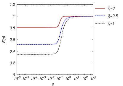
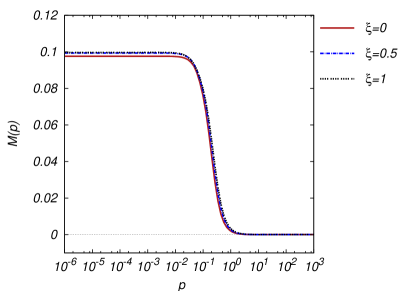
Figure 3: Fermion propagator in different covariant gauges. Solid line corresponds to $\xi=0$, dot-dashed line to $\xi=0.5$ and dotted line to $\xi=1$. Upper panel: Wavefunction renormalization $F(p)$. Lower panel: Mass function $M(p)$. The scale of the curves is set by the value $e^{2}=1$.

However, the fact remains that an LKFT for the fermion propagator as well as the 3-point vertex itself must conspire in such a manner as to yield a full 3-point vertex which would render physical observables independent of the gauge parameter, no matter what gauge we choose to work with. Precisely with this idea in mind, we presented the construction of the vertex in QED₄ in the previous section. We now ask ourselves whether the same form of the vertex would be sufficient to implement gauge invariance in three space-time dimensions. This implies finding ${\mathbf{a}}_{i}$ in $d=3$ dimensions. For $d=3$, one loop perturbative calculation of the transverse fermion-boson vertex in an arbitrary covariant gauge comes out to be

$$\Gamma^{\mu}_{T}(k,p) \stackrel{{\scriptstyle k^{2}>>p^{2}}}{{=}} -\frac{\alpha\xi\pi}{8p}\;\left[\gamma^{\mu}-\frac{k^{\mu}{\not\!k}}{k^{2}}\right]\;.$$ (19)

Interestingly, just as for $d=4$, we again have :

$${\mathbf{a}}_{3}^{3}+{\mathbf{a}}_{6}^{3} = \frac{1}{2}$$ (20)

in 3-dimensions. Similarly, the condition for the multiplicative renormalizability translates as the one of LKFT for the fermion propagator. Therefore, we now proceed to solve the gap equation in QED3 by employing the same form of the vertex as for QED4. Our starting point is to explore the configuration space of ${\mathbf{a}}_{2}$ and ${\mathbf{a}}_{6}$ in the Landau gauge. Then, we change the gauge parameter infinitesimally and repeat the same exercise. We look for the domain in the ${\mathbf{a}}_{2}/{\mathbf{a}}_{6}$-plane for which the difference of the condensate,

$$\delta_{\xi}=\langle\bar{\psi}\psi\rangle_{\xi}-\langle\bar{\psi}\psi\rangle_{\xi=0}\;,$$ (21)

is minimal. This is illustrated in Fig. 2. Within our numerical accuracy, different surfaces for fixed $\xi$ intersect along a line parameterized by

$${\mathbf{a}}_{2}^{3} = 3.81-7.6\ {\mathbf{a}}_{6}^{3}\;.$$ (22)

Thus, there is a family of vertex ansätze which yield a gauge invariant value of the condensate! Below we carry out a study of DCSB and confinement by selecting one member of this family of vertices. A priori, there is no guarantee that gauge independent DCSB should imply gauge independent confinement or vice versa.

III.1 DCSB

In order to make contact with our studies in QED4, we select the value of ${\mathbf{a}}_{2}^{3}=2.75$ and define our vertex by fixing ${\mathbf{a}}_{6}$ according to Eq. (22). With the choice of this vertex, we solve the gap equation in different gauges. Results are shown in Fig 3.

The mass functions change only slightly, whereas the variation in $F(p)$ is more noticeable. These changes conspire with each other to render the chiral fermion condensate gauge independent. We carry out a comparison with the same quantity obtained from the Curtis-Pennington Curtis:90 vertex as well as the Burden-Roberts vertex Burden:1991 . The results have been plotted in Fig .4, which clearly demonstrate the superiority of our proposal over the previous similar efforts for the de-construction of this Green function.

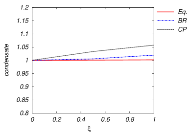
Figure 4: Gauge dependence of the chiral quark condensate for QED3. We compare our proposal against the ones by Burden-Roberts as well as Curtis-Pennington.

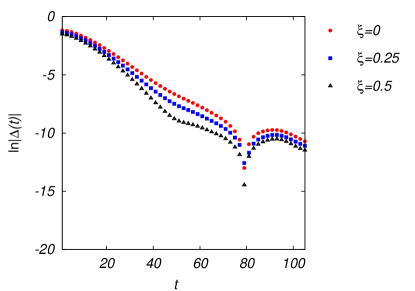
Figure 5: Spatially averaged Schwinger function in different gauges. Solid pentagons correspond to $\xi=0$, solid diamonds to $\xi=0.25$ and solid squares to $\xi=0.5$. Oscillations are inferred from the periodic peaks, which signal confinement. Position of the first dip is an order parameter for confinement. It is gauge invariant for our construction of the interaction.

III.2 Confinement

Confinement can be realized through the violation of the axiom of reflection positivity. For the fermion propagator, breach of the said axiom entails that the elementary excitation described by $S_{F}(p)$ cannot appear in the Hilbert space of observables. Confinement in QED3 can be explored through the positivity of the spatially averaged Schwinger function

$$\Delta(t)=\int d^{2}x\int\frac{d^{3}p}{(2\pi)^{3}}e^{ip\cdot x}\sigma_{s}(p^{2})\;,$$ (23)

which we construct from the solutions shown in Fig. 3. In Fig. 5 we display the logarithm of the absolute value of $\Delta(t)$ in different gauges. An oscillatory behavior of this function is revealed by the pronounced periodic peaks. This implies that $\Delta(t)$ is not positive definite and thus confinement is realized. The corresponding propagator possesses a pair of complex conjugated mass poles Krein:92 . Denoting $t_{c}$ the position of the first oscillation, $\nu=1/t_{c}$ serves as an order parameter for confinement Hawes:94 ; Bashir:05 ; Bashir:09 . Noticeably, $\nu$ is the same in all gauges, within our numerical accuracy. Thus confinement too has come out to be gauge independent with our choice of the fermion-boson vertex.

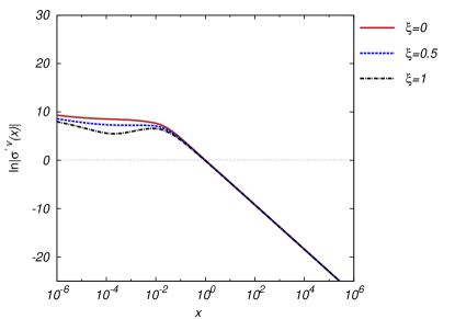
Figure 6: The first derivative of $\sigma_{v}(x)$ in various gauges. The maximum developed by all these functions is the order parameter, which is the same in all gauges within our numerical accuracy.

An alternative view of confinement stems from the fact that any function with an inflection point must violate the axiom of reflection positivity Bashir:09 ; Hofmann:10 ; Hofmann:11 . Let $x=p^{2}$. The above statement then implies that if there exists a point $x_{c}>0$ such that

$$\left.\frac{d^{2}}{dx^{2}}\sigma_{v}(x)\right|_{x=x_{c}}=0\;,$$ (24)

then the propagator describes a confined excitation, and $x_{c}$ plays the role of an order parameter for confinement. In Fig. 6, we plot the logarithm of the first derivative of $\sigma_{v}(x)$ in different gauges. We observe that all these curves develop a maximum at the same point $x_{c}$, which again means that there is confinement, and the corresponding order parameter is independent of choice of the covariant gauge $\xi$.

IV Concluding Remarks

In this article, building upon the proposal put forward in Bashir:thesis , we employ a simple form (e.g., it is independent of the photon momentum $q$) for the fermion-boson vertex in arbitrary dimensions. In 4-dimensions, it ensures WTI is satisfied, massless fermion propagator is multiplicatively renormalizable, one loop perturbation theory is recovered in the asymptotic limit $k^{2}>>p^{2}$, charge conjugation and parity properties of the vertex are respected and gauge independent value of critical electromagnetic coupling is achieved below which chiral symmetry is restored. This construction involves two free parameters which are momentum and gauge independent. However, the price we pay for ignoring the photon momentum dependence in this vertex ansatz is that these parameters naturally depend upon the dimension of space-time we choose to work with. We demonstrate that the same simple form of the vertex is able to render the order parameters for DCSB and confinement gauge invariant also in qQED3. We provide explicit comparisons with earlier proposals such as the Curtis-Pennington vertex (designed for $d=4$) as well as the Burden-Roberts vertex (constructed for $d=3$) to bring out the fact that our construction offers a marked improvement.

This is a first step in our intent to provide a unified truncation scheme for different gauge theories and a large body of associated physical observables. A natural next step is to extend our ideas to the SDE study of QCD. As mentioned before, an improved understanding of hadronic masses invokes additional structures in the fermion-boson vertex involving anomalous electromagnetic and chromomagnetic moments for dynamically massive quarks in the infrared. However, as a word of caution, one should remember that QCD is markedly more involved than QED3 as well as QED4. In covariant gauge QCD, ghosts play a vital role for its infrared dynamics, at least in the Landau gauge. Naturally, the ghost-gluon interaction also enters into the picture and one has to take into account the resulting complications with appropriate care. This work is in progress.

- (1) K. Higashijima, Phys. Rev. D 29, 1228 (1984).
- (2) V.A. Miransky, Phys. Lett. B 165, 401 (1985).
- (3) C.D. Roberts and A.G. Williams Prog. Part. Nucl. Phys. 33, 477 (1994).
- (4) C.S. Fischer, J. Phys. G 32, R253 (2006).
- (5) A. Bashir and A. Raya, ”Gauge symmetry and its implications for the Schwinger-Dyson equations”, published in the Trends in Boson Research, edited by A.V. Ling (Nova Science Publishers, New York, 2006).
- (6) R. Alkofer, C.S. Fischer, Annals Phys. 324, 106 (2009).
- (7) P. Maris and C.D. Roberts, Phys. Rev. C 56, 3369 (1997).
- (8) P. Maris and P.C. Tandy, Phys. Rev. C 62, 055204 (2000).
- (9) P. Maris and P.C. Tandy, Phys. Rev. C 65, 045211 (2002).
- (10) C-R. Ji and P. Maris, Phys. Rev. D 64, 014032 (2001).
- (11) P. Maris and P.C. Tandy, Phys. Rev. C 60, 055214 (1999).
- (12) D. Jarecke, P. Maris and P.C. Tandy Phys. Rev. C 67, 035202 (2003).
- (13) P. Maris, PiN Newslett. 16, 213 (2002).
- (14) S.R. Cotanch and P. Maris, Phys. Rev. D 66 116010 (2002).
- (15) L.X. Gutiérrez-Guerrero, A. Bashir, I.C. Clöet and C.D. Roberts, Phys. Rev. C 81, 065202 (2010).
- (16) H.L.L. Roberts, C.D. Roberts, A. Bashir, L.X. Gutiérrez-Guerrero, P.C. Tandy, Phys. Rev. C 82, 065202 (2010).
- (17) T. Nguyen, A. Bashir, C.D. Roberts, P.C. Tandy, Phys. Rev. C 83, 062201 (2011).
- (18) L. Chang, C.D. Roberts, Phys. Rev. Lett. 103, 081601 (2009).
- (19) L. Chang, Y-X. Liu, C.D. Roberts, Phys. Rev. Lett. 106, 072001 (2011).
- (20) A. Bashir, Y. Concha-Sánchez and R. Delbourgo, Phys. Rev. D 76 065009 (2007).
- (21) A. Bashir, Y. Concha-Sánchez, R. Delbourgo and M.E. Tejeda-Yeomans, Phys. Rev. D 80, 045007 (2009).
- (22) A. Bashir, Y. Concha-Sánchez, M.E. Tejeda-Yeomans, J.J. Toscano, Mod. Phys. Lett. A 25, 3145 (2010).
- (23) J.S. Ball and T. W. Chiu, Phys. Rev. D 22, 2542 (1980).
- (24) D.C. Curtis and M.R. Pennington, Phys. Rev. D 42, 4165 (1990).
- (25) A. Bashir and M.R. Pennington, Phys. Rev. D 50, 7679 (1994).
- (26) A. Bashir and M.R. Pennington, Phys. Rev. D 53, 4694 (1996).
- (27) A. Kizilersu, M. Reenders and M.R. Pennington, Phys. Rev. D 52, 1242 (1995).
- (28) A. Kizilersu and M.R. Pennington, Phys. Rev. D 79, 125020, (2009).
- (29) A. Bashir, C. Calcáneo-Roldan, L.X. Gutiérrez-Guerrero, and M.E. Tejeda-Yeomans, Phys. Rev. D 83, 033003 (2011).
- (30) C.J. Burden and C.D. Roberts, Phys. Rev. D 47, 5581 (1993).
- (31) Z. Dong, H.J. Munczek and C.D. Roberts, Phys. Lett. B 333, 536 (1994).
- (32) A. Bashir, A. Kizilersu and M.R. Pennington, Phys. Rev. D 57, 1242 (1998).
- (33) A. Bashir and A. Raya, Phys. Rev. D 64, 105001 (2001).
- (34) A. Bashir and R. Delbourgo, J. Phys. A 37, 6587 (2004).
- (35) J-I. Skullerud, P.O. Bowman, A. Kizilersu, D.B. Leinweber and A.G. Williams JHEP 04, 047 (2003).
- (36) A. Kizilersu, D.B. Leinweber, J-I. Skullerud and A.G. Williams, Eur. Phys. J. C 50, 871 (2007).
- (37) A.C. Aguilar and J. Papavassiliou, Phys. Rev. D 83, 014013 (2011).
- (38) A. Bashir, Constructing Vertices in QED, Ph.D. Thesis, Durham University, (1995).
- (39) A. Bashir, A. Huet and A. Raya, Phys. Rev. D66, 025029 (2002).
- (40) A. Bashir, A. Kizilersu, M.R. Pennington, Phys. Rev. D 57, 1242 (1998).
- (41) A. Bashir, A. Kizilersu and M.R. Pennington, Analytic form of the One-Loop Vertex and of the Two-Loop Fermion Propagator in 3-Dimensional massless QED, ADP-99-8/T353, DTP-99/76, Preprint: arXiv:hep-ph/9907418.
- (42) A.I. Davydychev, P. Osland and L. Saks Phys. Rev. D 63, 014022 (2000).
- (43) R. Delbourgo and A. Salam, Phys. Rev. 135, 1398 (1964).
- (44) R. Delbourgo and P. West, J. Phys. A 10, 1049 (1977).
- (45) R. Delbourgo and P. West, Phys. Lett. B 72, 96 (1977).
- (46) R. Delbourgo, Nuovo Cim. A 49, 484 (1979).
- (47) R. Delbourgo, B.W. Keck and C.N. Parker, J. Phys. A 14, 921 (1981).
- (48) G. Thompson and R. Zhang, Phys. Rev. D 35, 631 (1987).
- (49) C.N. Parker, J. Phys. A 17, 2873 (1984).
- (50) R. Delbourgo and R. Zhang, J. Phys. A 17, 3593 (1984).
- (51) C.J. Burden and C.D. Roberts, Phys. Rev. D 44, 540 (1991).
- (52) R. Pisarski, Phys. Rev. D 29, 2423 (1984).
- (53) T. Appelquist, M.J. Bowick, E. Cohler and L.C.R. Wijewardhana, Phys. Rev. Lett. 55, 1715 (1985).
- (54) M.R. Pennington and D. Walsh, Phys. Lett. B 253, 246 (1991).
- (55) D.C. Curtis, M.R. Pennington and D. Walsh, Phys. Lett. B 295, 313-319 (1992).
- (56) S.J. Hands, J.B. Kogut, C.G. Strouthos, Nucl. Phys. B 645, 321 (2002).
- (57) S.J. Hands, J.B. Kogut, L. Scorzato, C.G. Strouthos, Phys. Rev. B 70, 104501 (2004).
- (58) A. Bashir, A. Raya, I.C. Clöet and C.D. Roberts, Phys. Rev. C 78, 055201 (2008).
- (59) H. Feng, W. Sun, D. He and H. Zong, Phys. Lett. B 661, 57 (2008).
- (60) T. Goecke, C.S. Fischer and R. Williams, Phys. Rev. B 79, 064513 (2009).
- (61) H. Feng, M. He, W. Sun, H. Zong, Phys. Lett. B 688, 178 (2010).
- (62) W. Armour, John B. Kogut, C. Strouthos Phys. Rev. D 82, 014503 (2010).
- (63) P.M. Lo and E.S. Swanson, Phys. Rev. D 83, 065006 (2011).
- (64) J.A. Bonnet, C.S. Fischer and R. Williams, Effects of Anisotropy in from Dyson-Schwinger equations in a box e-Print: arXiv:1103.1578 [hep-ph].
- (65) M. Franz and Z. Tesanovic, Phys. Rev. Lett. 87, 257003 (2001).
- (66) M. Franz, Z. Tesanovic and O. Vafek, Phys. Rev. B 66, 054535 (2002).
- (67) Z. Tesanovic, O. Vafek and M. Franz, Phys. Rev. B 65, 180511 (2002).
- (68) I.F. Herbut, Phys. Rev. B 66, 094504 (2002).
- (69) I.O. Thomas and S. Hands, Phys. Rev. B 75, 134516 (2007).
- (70) K.S. Novoselov, A. K. Geim, S.V. Morozov, D. Jiang, M.I. Katsnelson, I.V. Grigorieva, S.V. Dubonos and A.A. Firsov, Nature 438, 197 (2005).
- (71) V.P. Gusynin, S.G. Sharapov and J.P. Carbotte, Int. J. Mod. Phys. B 21, 4611 (2007).
- (72) Riazuddin, Dirac equation for quasi-particles in graphene in an external electromagnetic field and chiral anomaly. e-Print: arXiv:1105.5956 [cond-mat.mes-hall].
- (73) L.D. Landau and I.M. Khalatnikov, Sov. Phys. JETP 2, 69 (1956), Zh. Eksp. Teor. Fiz. 29, 89 (1955).
- (74) E.S. Fradkin, Zh. Eksp. Teor. Fiz. 29, 258 (1955).
- (75) K. Johnson and B. Zumino, Phys. Rev. Lett. 3, 351 (1959).
- (76) B. Zumino, J. Math. Phys. 1, 1 (1960).
- (77) C. J. Burden, J. Praschifka, and C. D. Roberts, Phys. Rev. D46, 2695 (1992).
- (78) A. Bashir and A. Raya, Few-Body Syst. 41, 185 (2007).
- (79) A. Bashir, Phys. Lett. B491, 280 (2000).
- (80) A. Bashir and A. Raya, Phys. Rev. D66, 105005 (2002).
- (81) A. Bashir and A. Raya, Nucl. Phys. B709, 307 (2005).
- (82) A. Bashir, A. Raya, S. Sánchez-Madrigal, and C.D. Roberts, Few-Body Syst. 46, 229 (2009).
- (83) A. Bashir, A. Raya, and S. Sánchez-Madrigal, J. Phys. A41, 505401 (2008)
- (84) C.P. Hofmann, A. Raya, and Saúl Sánchez-Madrigal, Phys. Rev. D 82, 096011 (2010).
- (85) C.P. Hofmann, A. Raya, and Saúl Sánchez-Madrigal, J. Phys. Conf. Ser. 287, 012028 (2011).
- (86) G. Krein, C.D. Roberts and A.G. Williams, Int. J. Mod. Phys. A7, 5607 (1992).
- (87) F.T. Hawes, C.D. Roberts and A.G. Williams, Phys. Rev. D 49, 4683 (1994).