Department of Optics

Faculty of Natural Sciences

Palacký University

Olomouc, Czech Republic

Quantum properties of

superposition states,

squeezed states, and of some

parametric processes

Author: Faisal Aly Aly El-Orany

Doctoral Thesis

Branch: Optics and Optoelectronics

Supervisor: Prof. RNDr. Jan Peřina, DrSc.

Olomouc, 2001

Acknowledgments

First of all, I would like to start this thesis by passing my thanks to my supervisor, Professor Jan Peřina, under his supervision I worked more than three years; I thank him for collaboration in the most important and beautiful period of my life, I will never forget how much he was kind to me. I am very gratitude to him for long discussions and suggestions of interesting problems in nonlinear optics. This work could not be done in the present form without the support of all the members of the Department of Optics of Palacký University.

My warm thanks come next to Professor Mohamed Sebawe Abdalla from the Mathematics Department, College of Science, King Saud University, Riyadh, Saudi Arabia, for his suggestions of several problems and helping in some cases in the calculations. I wish to thank him for everything he did for me from the earlier days when I started to be engaged with quantum optics.

I would like to thank sincerely Professor Vlasta Peřinová for many discussions, support, advise as well as supply with some articles. My acknowledge extends to Dr. Jaromír Křepelka for many numerical advises.

I am obliged much to my mother, brothers and sister, I missed them too much, although they are always with me, and to my wife and son who give beautiful meaning to my life, and support me and are patient with me.

Chapter 1 Introduction

The failure of classical mechanics to account for many experimental results such as the stability of atoms and matter, blackbody radiation, etc. led physicists to the realization of new tool to deal with these problems and thus quantum mechanics came to the vicinity of life at the beginning of the last century. Indeed, quantum mechanics is the one of the crowning achievements of modern physics where the quantized electromagnetic field is supported by the experimental observations of nonclassical states of the radiation field, e.g. squeezed states, sub-Poissonian photon statistics and photon antibunching. Nowadays, quantum optics, the union of quantum field theory and physical optics, is undergoing a time of revolutionary change. The subject has evolved from early studies on the coherence properties of radiation to the laser in the modern areas of study involving, e.g., the role of squeezed states of the radiation field and atomic coherence in quenching quantum noise in interferometry and optical amplifiers. Furthermore, quantum optics provides a powerful new probe for addressing fundamental issues of quantum mechanics such as complementarity, hidden variables, and other aspects central to the foundations of quantum physics and philosophy.

For the description of a quantum system, the concept of state is used, which is the same, a wave function, a state vector or a density matrix containing the information about the possible results of measurement on the system. Quantum optics has statistical origin and therefore the state of a quantum system contains all information necessary to completely determine its statistics (the probabilistic nature of a quantum system). Among the wide variety of possible radiation-field states, there are some fundamental types that play a special role in quantum optics. Strictly speaking, there are three types of these states which are widely used, namely, coherent, number and squeezed states. Following the development of the quantum theory of radiation and with the advent of the laser, the coherent states of the field, that mostly describe a classical electromagnetic field, were widely studied. Indeed, these states are more appropriate basis for many optical fields. However, number states are purely nonclassical states and they are a useful representation of high-energy photons. However, there are experimental difficulties which have prevented the generation of photon number states with more than a small number of photons. Despite this the number states of the electromagnetic field have been used as a basis for several problems in quantum optics including some laser theories. The squeezed states (i.e. the states of light with reduced fluctuations in one quadrature below the level associated with the vacuum state) are very important owing to their potential applications, e.g. in the optical communication systems, interferometric techniques, and in an optical waveguide tap. Furthermore, squeezed states have been seen in several laboratories. In addition to these states, several quantum states in the literature have appeared, in particular those which are connected with the superposition principle. Using such principle, in the first part of this thesis, we will develop new class of states which are superposition of squeezed and displaced number states. In fact, this class of states generalizes some considerable results given in the literature. We close this part by giving an example of multidimensional squeeze operator which is more general than usually used.

On the other hand, nonlinear optics (NLO) has become a very important subfield of optics since its inception over 40 years ago. The origin of this branch is the study of the phenomena that occur as a consequence of the modification of the optical properties of a material system by the presence of light. The impact of NLO on science and technology has been twofold. First, it has enhanced our understanding of fundamental light-matter interactions. Second, it has been a deriving force in the rejuvenation of optical technology for several areas of science and engineering. For example, NLO provides the key to many developments, e.g. the advent of telecommunications using optical fibers, carrying information on a laser beam in the process of communication, storage, retrieval, printing or sensing, and there are increasing efforts to achieve ever greater data-processing capabilities. One of the most promising devices in NLO is the nonlinear directional coupler that consists of two or more parallel optical waveguides fabricated from some nonlinear material. Both waveguides are placed close enough to permit flux-dependent transfer of energy between them. This flux transfer can be controlled by the device design and the input flux as well. This device is experimentally implemented. Several models of this device will be investigated in the second part of this thesis.

As is well-known the quantum statistical properties of radiation present an important branch of modern physics with rapidly increasing applications in spectroscopy, quantum generators of radiation, optical communication, etc. Using these methods, quantum optics was able to predict many nonclassical phenomena, such as squeezing of vacuum fluctuations in field quadratures, antibunching of photons, sub-Poisson photon statistics exhibiting reduced photon-number fluctuations below the Poisson level of ideal laser light, quantum oscillations in photocount distributions, violation of various classical statistical inequalities, collapse and revival of atomic inversion, etc.

This doctoral thesis deals with investigating various quantum statistical aspects for new quantum states and for nonlinear directional couplers. The first part will be devoted to the static regime where we introduce the superposition of squeezed and displaced number states and discuss their quantum properties, phase properties and the influence of thermal noise on their behaviour. We conclude this part by giving an example of new type of multidimensional squeeze operator model which is more general than usually used and which includes two different squeezing mechanisms. The dynamical regime will be considered in the second part where we study the evolution of quantum states like coherent, number and thermal states in some nonlinear medium, such as nonlinear couplers. To achieve this goal in a systematic way we give first a survey of previous works in the literature related to our topic in chapter 2 and in chapter 3 we write down all mathematical relations controlling the quantum statistical properties of the models under discussion.

Chapter 2 Contemporary state of the problem

In this chapter, we display the most important relevant results in quantum optics which are used in our work. This will be done by throwing the light on the results of both squeezed light and the propagation of light in the nonlinear media.

2.1 Squeezed light

2.1.1 Squeezed states and squeezed superposition states

Squeezed states of the electromagnetic field are purely quantum states. They are defined through the relation

$$|\xi_{1},\alpha\rangle=\hat{D}(\alpha)\hat{S}(\xi_{1})|0\rangle,$$ (2.1.1)

where $|0\rangle$ is the vacuum state, $\hat{D}(\alpha)$  [1] and $\hat{S}(\xi_{1})$  [2] are displacement and squeeze operators which are given, respectively, by

$$\hat{D}(\alpha)=\exp(\hat{a}^{\dagger}\alpha-\hat{a}\alpha^{*}),$$ (2.1.2)

$$\hat{S}(\xi_{1})=\exp(\xi^{*}_{1}\hat{a}^{2}-\xi_{1}\hat{a}^{\dagger 2}),$$ (2.1.3)

where $\hat{a}$ and $\hat{a}^{\dagger}$ are annihilation and creation operators, respectively, and $\xi_{1}$ and $\alpha$ are complex parameters.

The significant feature for these states is that they can have less uncertainty in one quadrature than a coherent state. These states can exhibit a number of distinctly quantum features, such as sub-Poissonian statistics  [3, 4, 5], as well as they have no nonsingular representation in terms of the Glauber-Sudarshan $P$ distribution  [6]. It is important to refer that the concept of squeezed coherent states (SCS) have been applied to other quantum mechanical systems. For instance, they may play a role in increasing the sensitivity of a gravitational wave detector  [6]. SCS have appeared at the first time  [2] as a simple generalization of the well known minimum-uncertainty wavepackets. Authors of  [6, 7] have demonstrated further details concerning the properties of such states, or the so-called two-photon coherent states  [7].

A lot of efforts have been directed towards the methods of generating SCS. For example, we can mention, authors of  [8, 9, 10] have shown that squeezing may be generated in an optical four-wave mixing. Further progress has been done in papers  [11, 12], where the first experimental observations of squeezing were given in four-wave mixing in an atomic beam of Sodium vapor  [11] as well as in optical fibers  [12]. Particular attention was given to generate squeezed light in parametric amplifiers  [5, 13, 14, 15, 16], where the treatment of parametric oscillation and intracavity second harmonic generation provides the basis for subsequent calculations of squeezing in these systems. Furthermore, more activities have been focused on studying generation of SCS in: nondegenerate parametric oscillator  [17], optical bistability  [18, 19], and resonance fluorescence  [20, 21, 22]. For more complete information about SCS the reader can consult papers  [23, 24, 25].

The concept of superposition of quantum states has been extended by several authors to include SCS  [26, 27]. Authors of  [26] have introduced even and odd displaced squeezed states as a superposition of two vacuum squeezed displaced states. For such superposition the authors studied the higher-order squeezing with respect to the definition given by Hong and Mandel  [28]. Also it is interesting to refer to  [27] where extensive efforts have been done to introduce a superposition of set of SCS and the authors managed to calculate and discuss their quasiprobabality distribution functions as well as the generation scheme of such superposition states.

Squeezed and displaced number state (SDNS)  [29] is an energy eigenstate of a quantum harmonic oscillator which is displaced and then squeezed (it may also be called the generalized squeezed coherent state (GSCS)). For SDNS bunching and antibunching properties have been investigated  [30]. For more details about its properties, discussion as well as new methods for analytical investigation one can see paper  [31]. Further, for such a state, the most general form as well as the time-dependent expectation values, uncertainties of wave-functions and probability densities have been given in  [32] using the functional form for the squeeze and the time-displacement operators  [33]. Also we can mention that a special case of SDNS has been discussed in  [34] where these states have been treated from the point of view of non-diagonal $P$-representation. The authors have discussed the properties of the squeezed and displaced Fock states as generalized states and their discussion has been extended to the Glauber $R$-representation for the density operator as well as to the phase distribution. The physical interpretation of SDNS has been considered similarly to SCS  [29], in other words, SDNS is the coherent state formed due to two excitations on a particular number state. Also we can mention paper  [35] where squeezed (but not displaced) number state was produced.

We can also refer to several applications of SCS. For example, SCS have several potential applications, one, for instance, is in optical communication systems  [36]. Also the interferometric techniques may provide ways to detect very weak forces such as caused by gravitational radiation and may experience limitations on sensitivity due to quantum noise arising from photon counting and radiation pressure fluctuations  [37]. Another application is in an optical waveguide tap  [38] where it has been shown that a high signal-to-noise ratio may be obtained using SCS in an optical waveguide to tap a signal carrying waveguide.

2.1.2 Entangled squeezed states

Entangled states gain their feature from the quantum correlation between different quantum mechanical systems where the individual operator of the single system does not exhibit nonclassical effects, however, the compound system can exhibit such effects. To be more specific, if the measurement of an observable of the first system (say), for correlated system, is performed, this projects the other system into new states; otherwise the systems are uncorrelated. Squeezing property is the important phenomenon distinguishing well mechanism of correlation of systems, where squeezing can occur in combination of the quantum mechanical systems even if single systems are not themselves squeezed.

The most significant example for compound squeezing is related to the two-mode squeeze operator defined by an effective unitary operator as

$$\hat{S}(\xi_{2})=\exp(\xi^{*}_{2}\hat{a}^{\dagger}\hat{b}^{\dagger}-\xi_{2}\hat{a}\hat{b}),$$ (2.1.4)

where $\hat{a}$ and $\hat{b}$ are the annihilation operators of first and second modes respectively, and $\xi_{2}$ is a complex parameters. Expression (2.1.4) represent the evolution operator of the nondegenerate parametric amplifier with classical pumping and this operator can produce perfect squeezing only in the correlated states of two field modes. There are several models which have been given in the literature, e.g.  [39]– [43]. The aim of these articles is to examine the statistical properties for single- and compound-modes. Moreover, the ideas that quantum correlation can give rise to squeezing in the combination of system operators has been shown true for multimode squeezed states of light  [4, 5, 11, 39, 44, 45] and for dipole fluctuations in multimode squeezed states  [40].

2.1.3 Phase properties of squeezed states

In classical optics, the concepts of the intensity and phase of optical fields have a well-defined meaning. That is the electromagnetic field ($E$) associated with one mode, $E=A\exp(i\theta)$, has a well defined amplitude ($A$) and phase ($\theta$). This is not so simple in quantum optics where the mean photon number and the phase are represented by noncommuting operators and consequently they cannot be defined well simultaneously. In fact, the concept of phase is a controversional problem from the earlier days of quantum optics  [46, 47, 48]. In general there are three methods of treating this issue  [49]. The first one considers the phase as a physical quantity in analogy to position or momentum by representing it with a linear Hermitian phase operator. The second one involves c-number variables (real or complex) in phase spaces or their associated distribution functions, or ensembles of trajectories. The third one is the operational phase approach in which the phase information is inferred from the experimental data by analogy with the classical analysis of the experiment. Each approach has advantage and disadvantage points.

Squeezed states have phase sensitive noise properties and therefore several works have been devoted to follow such properties. We can mention that the authors of  [50] have investigated the fluctuation properties of squeezed states using a phase-operator formalism defined by Susskind and Glogower  [51]. They have shown that similarly as coherent states of high intensity approach a semiclassical number-phase uncertainty product, the squeezed states retain their quantum properties and their number-phase uncertainty relations are not minimized. However, the exact general results of the same technique have been obtained in  [52, 53] for single- and two-mode squeezed states. Indeed, these are mathematical treatment for the problem. Exact phase calculations for different definitions have been presented in  [54] showing that the measured-phase-operator formalism leads to contrasting behaviour compared with that based on the Susskind-Glogower or Hermitian-phase-operator formalisms. In the framework of Pegg-Barnett formalism  [55, 56, 57, 58] several works have been done treating not only single-mode squeezed states  [59, 60] but also two-mode squeezed states  [61]. The main results of these articles are: for single-mode squeezed states with non-zero displacement coherent amplitude, the phase distribution exhibits the bifurcation phenomenon or single peak-structure under certain conditions. However, it has been shown that the joint phase distribution for the two-mode squeezed vacuum depends only on the sum of the phases of the two modes, and that the sum of the two phases is locked to a certain value as the squeeze parameter increases  [62].

We refer to  [47, 48] where the investigation of phase properties of various quantum mechanical models in greater details have been given.

2.1.4 Squeezed states with thermal noise

It is worthwhile mentioning that squeezing of thermal radiation field has been already produced in a microwave Josephson-junction parametric amplifier  [63] where a thermal input field has been considered in a squeezing device and the generated field exhibits substantial noise reduction. The aim of such work is to generate nonclassical fields for interaction studies with Rydberg atoms in high-Q microwave cavities, where thermal noise in input fields is always large. Further, it has been suggested  [37] that interferometers for detection of gravitational waves could employ squeezing techniques in order to improve their resolution. Practically, these systems will inevitably experience thermal noise, so it is essential to be aware of the various representations of squeezed states and their physical interpretation  [64].

As a result of the fact that signal beams are usually accompanied by thermal noise, many authors concentrated on the studying of the influence of thermal noise on the behaviour of quantum states  [65]– [75]. Some of these studies give particular attention to the calculation of photon-counting distribution  [65]– [69]. This calculation basically depends on the Gaussian form of Wigner function. It has been shown that for large values of the squeeze parameter the photon-counting distribution is oscillating even for strong thermal noise. The quantum statistical properties of squeezed thermal light  [70]– [74], e.g. quadrature squeezing, second- and higher-order correlation functions, different representation for the density operator, and quasiprobability distribution functions, reveal that the degree of purity of the input thermal light is left unchanged by the subsequent squeezing and displacement processes. Moreover, an effective squeezing could be recognized under particular choice of the parameters and this fact is ensured by the behaviour of Glauber $P$-function which it no longer exists. For strong squeezing both squeezing properties and normalized correlation functions to all orders do not depend on the initial intensity of thermal field. The quantum phase distributions and variances of strong coherent and phase-squeezed states mixed with thermal light have been considered in  [75] showing that the effect of thermal noise on the coherent phase distribution becomes important only when the number of thermal photons is of the order of one-half ($(1/2)e^{-r}$, $r$ is the real squeeze parameter).

Here we may refer also to the squeezed thermal reservoir which has been studied in detail  [76]– [79]. One can see that the authors of ref.  [78] have shown for atom radiation in a squeezed thermal reservoir that the two quadratures of the atomic polarization are damped at different rates, which is consistent with the case of a squeezed vacuum reservoir. Furthermore, when the atom is driven by a coherent field, it has been found that the steady-state polarization depends on the relative phase of the squeezing and driving field. This phase dependence becomes less pronounced when the number of thermal photons increases. This behaviour suggests a number of novel applications, such as new schemes for optical bistability  [80]. Nevertheless, an objection against the reservoir technique can be given when an exact solution of the density matrix equation becomes unavailable even in the steady-state regime.

2.2 Light propagation

Classical optics describes quite successfully the propagation of laser light, both in free-space and inside a transparent medium. The reason is that in a coherent state of radiation, the electric and magnetic fields may be written in terms of their expectation values, and thus their propagation may be treated classically through the macroscopic Maxwell equations. The classical Maxwell equations permit the calculation of both the spatial progression and the temporal evolution of a propagating electromagnetic field, and treat the interaction of the field in a medium phenomenologically through the induced polarization. However, in quantum optics the simultaneous use of the Hamiltonian and the momentum operators yields operatorial spatial-temporal equations of motion for the electric and magnetic fields, having a form equivalent to that of the classical Maxwell equations and thus the quantum propagative phenomena can be rigorously described  [81, 82].

In this section we throw the light on two examples representing the propagation of light in media and which are frequently used in this thesis; namely, parametric processes and nonlinear directional coupler.

2.2.1 Parametric processes

There has been a great interest in the field of nonlinear optics for both the practical applications and the theoretical aspects of the nonlinear effects. Experiments in this field were made possible by the fact that the lasers with a sufficiently high output ($10^{5}$ to $10^{6}$ Watt/cm²) had become easily available  [83]. At this power level the nonlinear susceptibilities of certain media were producing observable effects  [84], e.g. such as the phenomena of parametric fluorescence and parametric oscillation  [85]. Indeed, linearity or nonlinearity is a property of the medium through which the light travels, rather than the property of the light itself. Light interacts with light via the medium. More precisely, the presence of an optical field modifies the properties of the medium which, in turn, modify another optical field or even the original field itself  [86]. For example, the study of the structure of crystals and molecules has long utilized the phenomena of light scattering from atoms or molecules having two energy levels. The frequency of the incident beam may then be shifted up or down, by an amount equal to the difference in the two energy levels of the scatterer. The resulting lower- and higher- frequency scattered waves are the Stokes and anti-Stokes components, respectively  [87]. However, in the coherent Raman effect the presence of a monochromatic light wave in a Raman active medium gives rise to parametric coupling between an optical vibrational mode and a mode of the radiation field which represents the scattered (Stokes) wave. In the case of Brillouin scattering a similar form of coupling holds, with the vibrational mode oscillating at an acoustic rather than an optical frequency  [5].

As was known the nonlinear processes in the quantum mechanical domain has led to the prediction and the observation of many quantum phenomena, e.g. squeezing of vacuum fluctuations and photon antibunching. In the heart of nonlinear optics there are two significant processes which have been attracted amount of study; namely, parametric frequency converter (PFC) and parametric amplifier (PA). PFC can be described by a process of exchanging photons between two optical fields of different frequencies: signal mode at frequency $\omega_{1}$ and idler mode at frequency $\omega_{2}$. This model can be applied to describe various optical phenomena, e.g. to find analogies between PFC and beam splitter  [88], two-level atom driven by a single mode of electromagnetic field  [89], and Raman scattering  [88, 90]. The quantum properties of PFC are discussed in  [91]. Further, some authors studied this model as the lossless linear coupler, e.g.  [92]- [95]. In this situation the model is considered to be represented by two electromagnetic waves which are guided inside the structure consisting of two adjacent and parallel waveguides; the linear exchange of energy between these two waveguides is established via the evanescent field  [96].

On the other hand, PA is designed in the most familiar form to amplify an oscillating signal by means of a particular coupling of the mode to a second mode of oscillation, the idler mode. The coupling parameter is made to oscillate with time in a way which gives rise to a steady increase of the energy in both the signal and idler modes  [5]. The importance of PA is related to the fact that it is the source for squeezed light  [7]. For example, degenerate and non-degenerate PA are sources for single-mode  [7] and two-mode  [39, 40, 41] squeezing of vacuum fluctuations, respectively.

The parametric process has been employed in experiments. For example, the fourth-order interference effects arise when pairs of photons produced in parametric down-conversion are injected into Michelson interferometers  [97]. However, the second-order interference is observed in the superposition of signal photons from two coherently pumped parametric down-conversions when the paths of the idler photons are aligned  [98]. Further, squeezed states of the electromagnetic field are generated by degenerate parametric down-conversion in optical cavity  [16] where noise reductions greater than $50\%$ relative to the vacuum noise level are observed in a balanced homodyne detector. Also, the observation of high-intensity sub-Poissonian light using the correlated "twin" beams generated by an optical parametric oscillator has been demonstrated  [99].

The optical processes involving the competition between PFC and PA are of interest from theoretical and experimental points of view, e.g. in three-mode interaction  [87, 100]. For these processes the quantum theory can be briefly reported as follows  [101]: The nonlinear interaction couples different photon modes and leads to energy transfer between modes. Photons in some modes may be annihilated, while those in the other modes created, and hence the photon distribution is disturbed. In every time the rate of energy transfer between the modes depends on the statistical properties of the light fields. Statistics is particularly important in this case for analyzing the results of experiments. As is expected the output field depends on the statistical nature of both the incident beams and the fluctuations in the medium. Moreover, the measurements of the statistical properties of the output field could yield information on the properties of the medium if those of the incident radiation are known.

2.2.2 Nonlinear directional coupler

In quantum optics many simple quantum systems have been examined from the point of view of completely quantum statistical description including not only amplitude and intensity (energy) development of such systems, but also higher-order moments and complete statistical behaviour. Such results have fundamental physical meaning for interpretation of quantum theory  [102] and they are useful for applications in optoelectronics and photonics as well. These results can be successfully transferred to more complicated and more practical systems, such as optical couplers composed of two or more waveguides connected linearly by means of evanescent waves. The waveguides can be linear or nonlinear employing various nonlinear optical processes, such as optical parametric processes, Kerr effect, Raman or Brillouin scattering, etc. Such devices play important role in optics, optoelectronics and photonics as switching and memory elements for all-optical devices (optical processors and computers). When one linear and the other nonlinear waveguides are employed, we have a nonlinear optical coupler producing nonclassical light in the nonlinear waveguide which can be controlled from the linear waveguide, i.e. one can control light by light. The generation and transmission of nonclassical light exhibiting squeezed vacuum fluctuations and/or sub-Poissonian photon statistics in nonlinear optical couplers can further be supported when all the waveguides are nonlinear. The possibility to generate and to transmit effectively nonclassical light in this way is interesting especially in optical communication and high-precision measurements where the reduction of quantum noise increases the precision.

Since the pioneering work on nonlinear couplers which has been done by Jensen  [103], a series of articles have been devoted to the study of this important optical device from both classical  [104]– [114] (using the coupled-mode theory) and quantal viewpoints  [115]– [135]. In the framework of quantum mechanics particular attention has been paid to quantum statistical properties in relation to quantum noise and generation and transmission of nonclassical light. Such generation and transmission of nonclassical light can be very effective as a consequence of using evanescent waves involved in the interaction. For a review of role of quantum statistical properties in nonlinear couplers, see  [136].

Chapter 3 Goals of the thesis

The main goal of the doctoral thesis is a study of quantum statistics for some static and dynamic regimes of nonlinear processes in quantum optics.

In the first part (static regime): 1- we want to develop a general class of quantum states as a superposition of displaced and squeezed number states. We study the quantum statistics for this class rigorously. We also investigate the effect of thermal noise on the properties of such class of states. Also we report the methods of generation for such superposition.
2- we want to give an example of new type of multidimensional squeeze operator model which is more general than usually used and which includes two different squeezing mechanisms. All basic properties related to this operator are discussed in greater details.

In the second part of this thesis we concentrate on studying the statistical properties of an optical field propagating within a nonlinear directional coupler. Our starting point is the Hamiltonian, which represents a nonlinear directional coupler. We assume one-passage propagation, so that losses in the beams have been neglected. In other cases they can be described in the standard quantum way in the form of interaction of light beams with reservoirs, as for instance described in  [137]. Moreover, we treat the problems of propagation in the Hamiltonian formalism assuming the energy of the system does not have directionality. However, in the case that all waves are propagating with the same velocity, time and space relate by the velocity of propagation $v$, $z=vt$. For all these models we investigate the effect of switching between the input modes and the outgoing fields from the coupler. We can consider three problems of light propagation in this device: 1- a symmetric directional coupler operating by nondegenerate parametric amplification.
2- nonlinear optical couplers composed of two nonlinear waveguides operating by the second subharmonic generation, which are coupled linearly through evanescent waves and nonlinearly through nondegenerate optical parametric interaction.
3- a nonlinear asymmetric directional coupler composed of a linear waveguide and a nonlinear waveguide operating by nondegenerate parametric amplification.

Chapter 4 Methods and tools of quantum theory used

In this chapter we review the quantum methods and tools for controlling the nonclassical phenomena, such as correlation function, quadratures squeezing, quasiprobability distribution function, photon-number distribution and phase distribution. Further, we do not describe a complete details for these methods and tools when they can be found in the standard text book. Moreover, we write down the formulae related to the dynamical regime where those of the static regime can be obtained by simply setting $t=0$ as a main tool the coherent-state technique is used.

4.1 Correlation functions

Antibunched and/or sub-Poissonian light is an example of nonclassical light and can be determined from a photocounting-correlation measurement. Starting with the experiment of Hanbury Brown and Twiss  [138], strong interest in the photon-counting statistics of optical fields began. Traditional diffraction and interference experiments and spectral measurements may be considered as being performed in the domain of one photon or linear optics. The theory of higher-order optical phenomena, described by higher-order correlation functions of the electromagnetic field, was founded by Glauber  [139], who introduced the measure of super-Poissonian statistics (classical phenomenon) and sub-Poissonian statistics (nonclassical phenomenon) of photons in any state. A state (of a single mode for convenience) which displays sub-Poisson statistics is characterized by the fact that the variance of the photon number $\langle(\triangle\hat{n}_{j}(t))^{2}\rangle$ is less than the average photon number $\langle\hat{n}_{j}(t)\rangle=\langle\hat{A}^{\dagger}_{j}(t)\hat{A}_{j}(t)\rangle$. This can be written by means of the normalized normal second-order correlation function as

$$g_{j}^{(2)}(t)=\frac{\langle\hat{a}_{j}^{\dagger 2}(t)\hat{a}_{j}^{2}(t)\rangle}{\langle\hat{a}_{j}^{\dagger}(t)\hat{a}_{j}(t)\rangle^{2}}\\ =1+\frac{\langle(\triangle\hat{n}_{j}(t))^{2}\rangle-\langle\hat{a}_{j}^{\dagger}(t)\hat{a}_{j}(t)\rangle}{\langle\hat{a}_{j}^{\dagger}(t)\hat{a}_{j}(t)\rangle^{2}},$$ (4.1.1)

where the subscript $j$ relates to the $j$th mode, and the photon number variances have the form

$$\langle(\triangle\hat{n}_{j}(t))^{2}\rangle=\langle(\hat{a}_{j}^{\dagger}(t)\hat{a}_{j}(t))^{2}\rangle-\langle\hat{a}_{j}^{\dagger}(t)\hat{a}_{j}(t)\rangle^{2}.$$ (4.1.2)

Then it holds that $g_{j}^{(2)}(t)<1$ for sub-Poissonian distribution of photons, $g_{j}^{(2)}(t)>1$ for super-Poissonian distribution of photons and when $g_{j}^{(2)}(t)=1$ Poissonian distribution occurs corresponding to a coherent state. Furthermore, for instance, the generation of sub-Poissonian light has been established in a semiconductor laser  [140] and in the microwave region using masers operating in the microscopic regime  [141]. An application of radiation exhibiting the sub-Poissonian statistics to optical communications has been considered in  [142].

On the other hand, it has been shown explicitly in  [143, 144] that sub-Poissonian photon statistics need not be associated with antibunching, but can be accompanied by bunching. However, within the framework of the classical theory, light cannot be antibunched, i.e. antibunched light is a manifestation of a quantum effect. The basic formula to study this phenomenon is the two-time normalized intensity correlation function  [144, 145]. For the $j$th mode, this function is defined by

$$g^{(2)}_{j}(t,t+\tau)=\frac{\langle\hat{a}^{\dagger}_{j}(t)\hat{a}^{\dagger}_{j}(t+\tau)\hat{a}_{j}(t+\tau)\hat{a}_{j}(t)\rangle}{\langle\hat{a}^{\dagger}_{j}(t)\hat{a}_{j}(t)\rangle\langle\hat{a}^{\dagger}_{j}(t+\tau)\hat{a}_{j}(t+\tau)\rangle}.$$ (4.1.3)

The importance of this function in the analysis of photon antibunching comes from the direct relation between this function and the joint detection probability of two photons, one at time $t$ and another at time $t+\tau$. It is clear that using (4.1.3) for $\tau\rightarrow 0$ as a definition of bunching properties, then the bunching/antibunching and super-/sub-Poissonian statistics are in one-to-one correspondence. More general definition of photon antibunching can be adopted  [144, 145] if $g^{(2)}_{j}(t,t+\tau)$ increases from its initial value at $\tau=0$. This can be represented in equivalent differential form, assuming that $g^{(2)}_{j}(t,t+\tau)$ is a well behaved function in $\tau$, as

$$K_{j}(t)=\frac{\partial g^{(2)}_{j}(t,t+\tau)}{\partial\tau}|_{\tau=0}>0;$$ (4.1.4)

photon bunching is given by the opposite condition ($K_{j}(t)<0$), otherwise the photons are unbunched. It is reasonable pointing out that antibunching and sub-Poissonian behaviour always accompany each other for the single-mode time-independent fields  [146].

Finally, we turn our attention to discuss the effect of intermodal correlation in terms of anticorrelations between different modes in the model. This can be done by two means. The first mean is given by introducing the photon-number operator $\hat{n}_{j,k}=\hat{A}^{\dagger}_{j}\hat{A}_{j}+\hat{A}^{\dagger}_{k}\hat{A}_{k}$ and calculating the quantity $\langle(\triangle W_{j,k})^{2}\rangle$=
$\langle:(\hat{n}_{j,k})^{2}:\rangle-\langle\hat{n}_{j,k}\rangle^{2}$, where : : denotes the normally ordered operator, i.e. creation operators $\hat{A}^{\dagger}_{j}$ are to the left of annihilation operators $\hat{A}_{j}$. The quantum anticorrelation effect is then characterized in terms of the variance of the photon number, which is less than the average of the photon number for nonclassical light, by negative values of $\langle(\triangle W_{j,k})^{2}\rangle$, i.e. negative cross-correlation taken two times is stronger than the sum of quantum noise in single modes  [147]. The second way is based on violation of Cauchy-Schwarz inequality. The violation of Cauchy-Schwarz inequality can be observed in a two-photon interference experiment  [148]. Classically, Cauchy-Schwarz inequality has the form  [149]

$$\langle I_{1}I_{2}\rangle^{2}\leq\langle I^{2}_{1}\rangle\langle I^{2}_{2}\rangle,$$ (4.1.5)

where $I_{j},j=1,2$ are classical intensities of light measured by different detectors in a double-beam experiment. In quantum theory, the deviation from this classical inequality can be represented by the factor  [150]

$$I_{j,k}=\frac{[\langle\hat{A}^{\dagger 2}_{j}\hat{A}^{2}_{j}\rangle\langle\hat{A}^{\dagger 2}_{k}\hat{A}^{2}_{k}\rangle]^{\frac{1}{2}}}{\langle\hat{A}^{\dagger}_{j}\hat{A}_{j}\hat{A}^{\dagger}_{k}\hat{A}_{k}\rangle}-1.$$ (4.1.6)

The negative values for the quantity $I_{j,k}$ mean that the intermodal correlation is larger than the correlation between the photons in the same mode  [43] and this indicates strong violation of the Cauchy-Schwarz inequality. Finally, anticorrelation between modes can be measured by detecting single modes separately by two photodetectors and correlating their outputs.

4.2 Quadrature squeezing

As we mentioned earlier, squeezed light possesses less noise than a coherent light in one of the field quadratures and can exhibit a number of features having no classical analogue. This light can be measured by homodyne detection where the signal is superimposed on a strong coherent beam of the local oscillator.

There are several definitions for squeezing, e.g. standard squeezing  [151], amplitude-squared squeezing  [152], two-mode squeezing  [153], higher-order squeezing  [154], principal squeezing  [155], etc. Of course, the quantum mechanical systems can exhibit different types of squeezing at the same time. It has been shown that when a beam of light propagates through a nonlinear crystal, in the process of generation of the second harmonic, the fundamental mode becomes squeezed in the sense of standard  [151] as well as amplitude-squared squeezing  [152]. Further, the parametric amplifier in a cavity can ideally produce squeezed light with characteristics akin to the single and two modes when operating in degenerate and non-degenerate regimes, respectively  [153].

In this thesis we investigate single-mode, two-mode and three-mode squeezing on the basis of the two quadratures $\hat{X}_{n}$ and $\hat{Y}_{n}$ (where the subscript $n$ takes on 1,2,3 associated with the single-, two- and three-mode squeezing) which are related to the conjugate electric and magnetic field operators $\hat{E}$ and $\hat{H}$. They are defined in the standard way. Assuming that these two quadrature operators satisfy the following commutation relation

$$\left[\hat{X}_{n},\hat{Y}_{n}\right]=C,$$ (4.2.1)

where $C$ is a c-number specified later, the following uncertainty relation holds

$$\langle(\triangle\hat{X}_{n})^{2}\rangle\langle(\triangle\hat{Y}_{n})^{2}\rangle\geq\frac{|C|^{2}}{4},$$ (4.2.2)

where $\langle(\triangle\hat{X}_{n})^{2}\rangle=\langle\hat{X}_{n}^{2}\rangle-\langle\hat{X}_{n}\rangle^{2}$ is the variance. Therefore, we can say that the model possesses $X_{n}$-quadrature squeezing if the $S_{n}$-factor  [156],

$$S_{n}=\langle(\triangle\hat{X}_{n}(t))^{2}\rangle-0.5|C|,$$

$$=\frac{\langle(\triangle\hat{X}_{n}(t))^{2}\rangle-0.5|C|}{0.5|C|},$$ (4.2.3)

satisfies the inequality $-1\leq S_{n}<0$. Similar expression for the $Y_{n}$-quadrature ($Q_{n}$-parameter) can be obtained.

For example, the two quadratures of three-mode squeezing are defined as

$$\hat{X}_{3}(t)=\frac{1}{2}[\hat{A}_{1}(t)+\hat{A}_{2}(t)+\hat{A}_{3}(t)+\hat{A}_{1}^{\dagger}(t)+\hat{A}_{2}^{\dagger}(t)+\hat{A}_{3}^{\dagger}(t)],$$ (4.2.4)

$$\hat{Y}_{3}(t)=\frac{1}{2i}[\hat{A}_{1}(t)+\hat{A}_{2}(t)+\hat{A}_{3}(t)-\hat{A}_{1}^{\dagger}(t)-\hat{A}_{2}^{\dagger}(t)-\hat{A}_{3}^{\dagger}(t)].$$ (4.2.5)

The expressions for the single-mode and two-mode squeezing can be obtained easily from (4.2.4) and (4.2.5) by dropping the operators of absent mode, e.g. for the 1st mode, single-mode squeezing can be obtained by setting the operators of 2nd and 3rd modes equal zero. It should be taken into account that $C=\frac{1}{2},1,\frac{3}{2}$ corresponding to the single-mode, two-mode and three-mode squeezing, respectively.

4.3 Quasiprobability functions

Evaluation of various time-dependent mode observables is most conveniently achieved with the aid of corresponding time-dependent characteristic functions, their normal, antinormal and symmetric forms, and the Fourier transforms of these characteristic functions (quasiprobability functions). All of these are related to the density matrix which provides a complete statistical description of the system. There are three types of quasiprobability functions: Wigner $W$-, Glauber $P$-, and Husimi $Q$-functions. These functions could be used also as crucial to describe the nonclassical effects of the system, e.g. one can employ the negative values of $W$-function, stretching of $Q$-function and high singularities in $P$-function. Furthermore, these functions are now accessible from measurements  [157].

Indeed, the detailed statistics of the coupled field modes can be obtained from several photon-counting experiments. Most often we are interested in the quantum statistics of either one mode which determine the ensemble averages of the observable of this mode, or the composite statistics of the compound modes which reflect their mutually correlated properties. That is why we consider in this thesis phase space distributions for the single- and compound-modes for different types of initial states.

The $s$-parametrized joint characteristic function for the compound system ($n$ modes) defined by

$$C^{(n)}(\underline{\zeta},t,s)={\rm Tr}\left\{\hat{\rho}(0)\exp\left[\sum_{j=1}^{n}(\zeta_{j}\hat{A}_{j}^{\dagger}(t)-\zeta_{j}^{*}\hat{A}_{j}(t)+\frac{s}{2}|\zeta_{j}|^{2})\right]\right\},$$ (4.3.1)

where $\hat{\rho}(0)$ is the initial density matrix for the system under consideration, $\underline{\zeta}=(\zeta_{1},\zeta_{2},...,\zeta_{n})$ is a set of parameters, and $s$ takes on values $1,0$ and $-1$ corresponding to normally, symmetrically and antinormally ordered characteristic functions, respectively.

Thus the $s$-parametrized joint quasiprobability functions are given by

$$W^{(n)}(\underline{\beta},t,s)=\frac{1}{\pi^{2n}}\underline{\int}C^{(n)}(\underline{\zeta},t,s)\prod_{j=1}^{n}\exp(\beta_{j}\zeta_{j}^{*}-\beta_{j}^{*}\zeta_{j})d^{2}\zeta_{j},$$ (4.3.2)

where $\underline{\beta}=(\beta_{1},\beta_{2},...,\beta_{n})$ are complex amplitudes and $\underline{\int}=\int...\int$ $n$-fold integral. When $s=1,0,-1$, equation (4.3.2) gives formally Glauber $P$-function, Wigner $W$-function and Husimi $Q$-function, respectively.

On the other hand, the $s$-parametrized quasiprobability functions for the single-mode can be attained by means of integrating $(n-1)$ times in the corresponding joint quasiprobability functions or by using the single-mode $s$-parametrized characteristic function. For instance, the characteristic function $C^{(1)}(\zeta_{1},t,s)$ for mode $\hat{A}_{1}$ (say) can be obtained from $C^{(n)}(\underline{\zeta},t,s)$ by simply setting $\zeta_{k}=0,\quad k=2,3,...,n$. Hence the $s$-parametrized single-mode quasiprobability can be derived by

$$W^{(1)}(\beta_{1},t,s)=\underline{\int}W^{(n)}(\underline{\beta},t,s)\prod_{j=2}^{n}d\beta_{j},$$ (4.3.3)

etc., or

$$W^{(1)}(\beta_{j},t,s)=\frac{1}{\pi^{2}}\int C^{(1)}(\zeta_{j},t,s)\exp(\beta_{j}\zeta_{j}^{*}-\beta_{j}^{*}\zeta_{j})d^{2}\zeta_{j}.$$ (4.3.4)

$C^{(1)}(\zeta_{j},t,s)$ in (4.3.4) is the $s$-parametrized characteristic function for single-mode. The superscripts (1) and (n) in the above equations stand for single-mode case and $n$-mode case, respectively.

The various moments of the bosonic operators for the system, using the characteristic functions and quasiprobability functions, in the normal form (N), antinormal form (A) and symmetrical form (S), corresponding to $s=1,-1,0$, respectively, can be obtained by

$$\langle\prod_{j=1}^{n}\hat{A}_{j}^{\dagger m_{j}}(t)\hat{A}_{j}^{n_{j}}(t)\rangle_{N,A,S}=\prod_{j=1}^{n}\frac{\partial^{m_{j}+n_{j}}}{\partial\zeta_{j}^{m_{j}}\partial(-\zeta_{j}^{*})^{n_{j}}}C^{(n)}(\underline{\zeta},s,t)_{s=1,-1,0}|_{\underline{\zeta}=\underline{\zeta}^{*}=0}$$

$$=\underline{\int}W^{(n)}(\underline{\beta},s,t)_{(s=1,-1,0)}\prod_{j=1}^{n}\beta_{j}^{*m_{j}}\beta_{j}^{n_{j}}d^{2}\beta_{j},$$ (4.3.5)

where $n_{j},m_{j}$ are positive integers. The formulae (4.3.5) are valid for the single mode and compound modes as well.

There are several applications of the quasiprobability function. We restrict ourselves to those of the single-mode case because the generalization to the multi-mode case is straightforward.

First, the degree of purity ${\rm Tr}\rho^{2}$ for any state can be evaluated with aid of the symmetrical characteristic function given by the relation

$${\rm Tr}(\rho^{2})=\frac{1}{\pi}\int|C(\zeta,s=0)|^{2}d^{2}\zeta.$$ (4.3.6)

One can find for a pure state ${\rm Tr}(\rho^{2})=1$ and for a mixed state ${\rm Tr}(\rho^{2})<1$. Also, the quasiprobability function can be used to calculate the matrix elements of $\hat{\rho}_{1}(t)$ in the $n$-quantum representation at time $t$ by means of the relation  [5]

$$\langle m|\hat{\rho}_{1}(t)|n_{1}\rangle=\int\frac{\beta^{m}_{1}\beta^{*n_{1}}_{1}}{\sqrt{n_{1}!m!}}W^{(1)}(\beta_{1},s=1,t)\exp(-|\beta_{1}|^{2})d^{2}\beta_{1}.$$ (4.3.7)

It is clear that this formula reduces to the photon-number distribution when $m=n_{1}$. Further, the photon-number distribution can be obtained also from the integral relation in terms of Wigner function of the specified mode and Laguerre polynomials as

$$P^{(1)}(n_{j},t)=\frac{2(-1)^{n_{j}}}{n_{j}!}\int W^{(1)}(\beta_{j},t)\exp(-2|\beta_{j}|^{2})L_{n_{j}}(4|\beta_{j}|^{2})d^{2}\beta_{j},$$ (4.3.8)

where $j$ denotes the mode under consideration and $W^{(1)}(\beta_{j},t)$ is the single mode Wigner function for the specified mode. Also quasiprobability functions can be used to investigate the phase distribution for the structure by integrating these functions over the radial variable  [46, 47, 48]

$$P(\theta,s,t)=\int_{0}^{\infty}W^{(1)}(\beta_{j},s,t)|\beta_{j}|d|\beta_{j}|,$$ (4.3.9)

where $\beta_{j}=|\beta_{j}|\exp(i\theta)$.

More details on the phase properties in terms of Pegg-Barnett formalism will be given in the following section.

4.4 Phase properties-Pegg-Barnett formalism

Here we give essential background for Pegg-Barnett  [55]– [58] phase formalism. This formalism is based on introducing a finite $(s+1)$-dimensional space $\Psi$ spanned by the number states $|0\rangle,|1\rangle,...,|s\rangle$. The physical variables (expectation values of Hermitian operators) are evaluated in the finite dimensional space $\Psi$ and at the final stage the limit $s\rightarrow\infty$ is taken. A complete orthonormal basis of $s+1$ states is defined on $\Psi$ as

$$|\Theta_{m}\rangle=\frac{1}{\sqrt{s+1}}\sum^{s}_{k=0}\exp(ik\Theta_{m})|k\rangle,$$ (4.4.1)

where

$$\Theta_{m}=\Theta_{0}+\frac{2\pi m}{s+1},\qquad m=0,1,...,s.$$ (4.4.2)

The value of $\Theta_{0}$ is arbitrary and defines a particular basis of $s+1$ mutually orthogonal states. The Hermitian phase operator is defined as

$$\hat{\Phi}_{\theta}=\sum^{s}_{m=0}\Theta_{m}|\Theta_{m}\rangle\langle\Theta_{m}|,$$ (4.4.3)

where the subscript shows the dependence on the choice of $\Theta_{0}$. The phase states (4.4.1) are eigenstates of the phase operator (4.4.3) with the eigenvalues $\Theta_{m}$ restricted to lie within a phase window between $\Theta_{0}$ and $2\pi+\Theta_{0}$. The expectation value of the phase operator (4.4.3) in a pure state $|\psi\rangle=\sum^{\infty}_{m=0}C_{m}|m\rangle$, where $C_{m}$ is the weighting coefficient including the normalization constant, is given by

$$\langle\psi|\hat{\Phi}_{\theta}|\psi\rangle=\sum^{s}_{m=0}\Theta_{m}|\langle\psi|\Theta_{m}\rangle|^{2}.$$ (4.4.4)

The density of phase states is $(s+1)/(2\pi)$, so the continuum phase distribution as $s$ tends to infinity is

$$\begin{array}[]{rl}P(\Theta)={\rm lim}_{s\rightarrow\infty}\frac{s+1}{2\pi}|\langle\Theta_{m}|\psi\rangle|^{2}\\ \\ =\frac{1}{2\pi}\sum_{m,m^{{}^{\prime}}=0}^{\infty}C_{m}C^{*}_{m^{{}^{\prime}}}\exp[i(m-m^{{}^{\prime}})\Theta],\end{array}$$ (4.4.8)

where $\Theta_{m}$ has been replaced by the continuous phase variable $\Theta$. As soon as the phase distribution $P(\Theta)$ is known, all the quantum-mechanical phase moments can be obtained as a classical integral over $\Theta$. One of the particular interesting quantities in the description of the phase is the phase variance determined by

$$\langle(\triangle\hat{\Phi})^{2}\rangle=\int\Theta^{2}P(\Theta)d\Theta-\left(\int\Theta P(\Theta)d\Theta\right)^{2}.$$ (4.4.9)

As is well known the mean photon number and the phase are conjugate quantities in this approach and consequently they obey the following uncertainty relation

$$\langle(\triangle\hat{\Phi})^{2}\rangle\langle(\triangle\hat{n})^{2}\rangle\geq\frac{1}{4}|\langle[\hat{n},\hat{\Phi}]\rangle|^{2}.$$ (4.4.10)

The number–phase commutator appearing on the right-hand side of (4.4.10) can be calculated for any physical state  [55]– [58] as

$$\langle[\hat{n},\hat{\Phi}]\rangle=i[1-2\pi P(\Theta_{0})].$$ (4.4.11)

In relation to (4.4.10), we can give the notion of the number and phase squeezing  [158, 159] through the relation

$$S_{n}=\frac{\langle(\triangle\hat{n})^{2}\rangle}{\frac{1}{2}|\langle[\hat{n},\hat{\Phi}]\rangle|}-1,$$ (4.4.12)

$$S_{\theta}=\frac{\langle(\triangle\hat{\Phi})^{2}\rangle}{\frac{1}{2}|\langle[\hat{n},\hat{\Phi}]\rangle|}-1.$$ (4.4.13)

The values of $-1$ in these equations means maximum squeezing of the photon number or the phase.

In this thesis we calculate the quantities given in this chapter for the models under discussion and then numerical simulations are performed using, e.g. Surfer or Matlab program.

Chapter 5 Scientific results and their analysis: part I (static regime)

In this part we investigate the quantum properties for a superposition of squeezed and displaced number states (SSDNS) without and with thermal noise. We suggest also a new type of multidimensional squeeze operator and discuss its properties in details.

5.1 Quantum statistical properties of superposition of squeezed and displaced number states

This section is devoted to study properties of superposition of squeezed and displaced number states (SSDNS) such as orthogonality property, wave function, photon-number distribution, quasiprobability functions and phase properties in terms of Pegg-Barnett formalism.

5.1.1 State formalism and some of its properties

Here we develop a general class of quantum states, as a result of a superposition between two quantum states, described as a single mode vibration of electromagnetic field which is on a sudden squeezed-plus-displaced by a collection of two displacements $180^{0}$ out of phase given as

$$|r,\alpha,n\rangle_{\epsilon}=\lambda_{\epsilon}[\hat{D}(\alpha)+\epsilon\hat{D}(-\alpha)]\hat{S}(r)|n\rangle,$$ (5.1.1)

where $\hat{D}(\alpha)$ and $\hat{S}(r)$ are the displacement and squeeze operators, given by (2.1.2) and (2.1.3), respectively, with $\xi_{1}=r$ and $\alpha$ are real; $\epsilon=|\epsilon|e^{{\rm i}\phi}$ is a parameter specified later on, $\phi$ is a phase; $|n\rangle$ is the number (Fock) state, and $\lambda_{\epsilon}$ is a normalization constant given as

$$|\lambda_{\epsilon}^{2}|^{-1}=1+|\epsilon|^{2}+2|\epsilon|\exp(-2t^{2}){\rm L}_{n}(4t^{2})\cos\phi,$$ (5.1.2)

where $t=\alpha e^{r}$, ${\rm L}_{n}(.)$ is the Laguerre polynomial. During the derivation of (5.1.2), we used the relations

$$\begin{array}[]{lr}\hat{D}^{\dagger}(\alpha)\hat{a}\hat{D}(\alpha)=\hat{a}+\alpha,\qquad\hat{S}^{\dagger}(r)\hat{a}\hat{S}(r)=\hat{a}C_{r}-\hat{a}^{\dagger}S_{r},\\ \hat{D}(\zeta)\hat{D}(\beta)=\hat{D}(\zeta+\beta)\exp[\frac{1}{2}(\zeta\beta^{*}-\zeta^{*}\beta)],\quad\hat{S}^{\dagger}(r)\hat{D}(\beta)\hat{S}(r)=\hat{D}(\beta C_{r}+\beta^{*}S_{r}),\end{array}$$ (5.1.5)

and the relation  [160]

$$\langle n|\hat{D}(t)|k\rangle=\left\{\begin{array}[]{rl}\sqrt{\frac{k!}{n!}}\exp(-\frac{t^{2}}{2})t^{n-k}{\rm L}^{n-k}_{k}(t^{2})&{\rm for}\;n\geq k,\\ \sqrt{\frac{n!}{k!}}\exp(-\frac{t^{2}}{2})(-t)^{k-n}{\rm L}^{k-n}_{n}(t^{2})&{\rm for}\;k\geq n,\end{array}\right.$$ (5.1.6)

where $C_{r}=\cosh r,S_{r}=\sinh r$; ${\rm L}^{\gamma}_{n}(.)$ is associated Laguerre polynomial. The same states (5.1.1) were investigated independently in [161].

The density matrix $\hat{\rho}$ of this state can be written as

$$\hat{\rho}=|\lambda_{\epsilon}|^{2}(\hat{\rho}_{M}+\hat{\rho}_{I}).$$ (5.1.7)

The part of the density matrix corresponding to the statistical mixture of two squeezed displaced number states is:

$$\hat{\rho}_{M}=\hat{D}(\alpha)\hat{S}(r)|n\rangle\langle n|\hat{S}^{\dagger}(r)\hat{D}^{\dagger}(\alpha)+|\epsilon|^{2}\hat{D}(-\alpha)\hat{S}(r)|n\rangle\langle n|\hat{S}^{\dagger}(r)\hat{D}^{\dagger}(-\alpha),$$ (5.1.8)

while the quantum interference part has the form

$$\hat{\rho}_{I}=\epsilon^{*}\hat{D}(\alpha)\hat{S}(r)|n\rangle\langle n|\hat{S}^{\dagger}(r)\hat{D}^{\dagger}(-\alpha)+\epsilon\hat{D}(-\alpha)\hat{S}(r)|n\rangle\langle n|\hat{S}^{\dagger}(r)\hat{D}^{\dagger}(\alpha).$$ (5.1.9)

This quantum interference part of the density matrix contains information about the quantum interference between component states $\hat{D}(\pm\alpha)\hat{S}(r)|n\rangle$ and this will be responsible for some interesting behaviour of the phase distribution, as we will see. For completeness, the physical interpretation of such states can be related to a superposition of coherent states formed due to two excitations on particularly excited harmonic oscillators  [29]. It is clear that these states enable us to obtain generalizations of some results given in the literature, e.g.  [70, 71, 73, 88, 162, 163, 164, 165, 166]. Firstly, the wavefunction of state (5.1.1) can be determined through  [31] as

$$\Psi^{(\epsilon)}_{n}(x,r,\alpha)=\langle x|r,\alpha,n\rangle_{\epsilon}=\lambda_{\epsilon}\frac{\partial^{n}}{\partial\mu^{n}}\int\langle x|\mu\rangle\langle\mu|[\hat{D}(\alpha)+\epsilon\hat{D}(-\alpha)]\hat{S}(r)\exp(\mu\hat{a}^{\dagger})|0\rangle\frac{d^{2}\mu}{2\pi},$$ (5.1.10)

where we have used the overcompleteness relation for coherent states; after substituting for the element $\langle x|\mu\rangle$ from [76] into (5.1.10) and using similar technique as in  [31], we arrive at (with $\alpha$ is real)

$$\begin{array}[]{rl}\Psi^{(\epsilon)}_{n}(x,r,\alpha)=\frac{\lambda_{\epsilon}e^{\frac{r}{2}}}{\sqrt{2^{n}n!}}(\frac{\omega}{\pi\hbar})^{\frac{1}{4}}\left\{\exp\left[-\frac{e^{2r}}{2}(x\sqrt{\frac{\omega}{\hbar}}-\sqrt{2}\alpha)^{2}\right]{\rm H}_{n}[e^{r}(x\sqrt{\frac{\omega}{\hbar}}-\sqrt{2}\alpha)]\right.\\ \\ +\epsilon\exp\left[-\frac{e^{2r}}{2}(x\sqrt{\frac{\omega}{\hbar}}+\sqrt{2}\alpha)^{2}\right]\left.{\rm H}_{n}[e^{r}(x\sqrt{\frac{\omega}{\hbar}}+\sqrt{2}\alpha)]\right\},\end{array}$$ (5.1.14)

where $\omega$ and $\hbar$ are frequency of the harmonic oscillator and Planck’s constant divided by $2\pi$; they appeared here as a result of using the wavefunction $\langle x|\beta\rangle$ when describing a coherent state of the harmonic oscillator in the coordinate representation in the derivation of (5.1.14).

The inner product of the ket $|r,\alpha,n\rangle_{\epsilon}$ with the bra ${}_{\epsilon^{\prime}}\langle r^{\prime},\alpha^{\prime},m|$ can be calculated using the wavefunction (5.1.14) through the relation

$${}_{\epsilon^{\prime}}\langle m,\alpha^{\prime},r^{\prime}|n,\alpha,r\rangle_{\epsilon}=\int_{-\infty}^{+\infty}dx\Psi^{(\epsilon^{\prime})*}_{m}(x,r^{\prime},\alpha^{\prime})\Psi^{(\epsilon)}_{n}(x,r,\alpha),$$ (5.1.15)

together with the identity  [167]

$$\begin{array}[]{rl}\sqrt{\frac{M}{\pi}}\int_{-\infty}^{+\infty}dx{\rm H}_{m}(x){\rm H}_{n}(\Lambda x+d)\exp(-Mx^{2}+cx)=\exp(\frac{c^{2}}{4M})\\ \\ \times(\sqrt{\frac{M-1}{M}})^{m}(\sqrt{\frac{M-\Lambda^{2}}{M}})^{n}\sum_{j=0}^{min(m,n)}\frac{n!m!}{j!(n-j)!(m-j)!}\\ \\ \times\left(\frac{2\Lambda}{\sqrt{(M-1)(M-\Lambda^{2})}}\right)^{j}{\rm H}_{m-j}\left(\frac{c}{2\sqrt{(M-1)M}}\right){\rm H}_{n-j}\left(\frac{c\Lambda+2dM}{2\sqrt{M(M-\Lambda)}}\right),\end{array}$$ (5.1.21)

as

$$\begin{array}[]{rl}_{\epsilon^{\prime}}\langle m,\alpha^{\prime},r^{\prime}|n,\alpha,r\rangle_{\epsilon}=\frac{\lambda_{\epsilon^{\prime}}\lambda_{\epsilon}(\frac{\tanh R}{2})^{\frac{m}{2}}}{\sqrt{n!m!\cosh R}}\sum_{j=0}^{min(m,n)}\frac{n!m![\frac{-\tanh R}{2}]^{\frac{(n-j)}{2}}}{j!(n-j)!(m-j)!}[\frac{2}{\sqrt{\sinh 2R}}]^{j}\\ \\ \times\left\{\exp[\frac{\tau^{2}_{1}}{2}(\tanh R-1)]{\rm H}_{n-j}(X_{1}){\rm H}_{m-j}(X_{2})[1+(-1)^{(n+m)}\epsilon^{\prime*}\epsilon]\right.\\ \\ \left.+\exp[\frac{\tau^{2}_{2}}{2}(\tanh R-1)]{\rm H}_{n-j}(Y_{1}){\rm H}_{m-j}(Y_{2})[\epsilon^{\prime*}+(-1)^{(n+m)}\epsilon]\right\}\end{array}$$ (5.1.27)

and

$$\begin{array}[]{rl}R=r-r^{\prime},\quad\tau_{1}=(\alpha-\alpha^{\prime})e^{r},\quad\tau_{2}=(\alpha+\alpha^{\prime})e^{r},\quad X_{1}=\frac{{\rm i}\tau_{1}e^{-R}}{\sqrt{\sinh 2R}},\\ X_{2}=\frac{\tau_{1}}{\sqrt{\sinh 2R}},\quad Y_{1}=\frac{{\rm i}\tau_{2}e^{-R}}{\sqrt{\sinh 2R}},\quad Y_{2}=\frac{\tau_{2}}{\sqrt{\sinh 2R}},\end{array}$$ (5.1.30)

where ${\rm H}_{m}(.)$ is the Hermite polynomial of order m. It is clear that for $\epsilon^{\prime}=-1,\epsilon=1$ and $n=m$ equation (5.1.27) vanishes, that is the inner product of two states, one from even subspace and the other from odd subspace, is zero. Here we assume that $\epsilon^{\prime}=\epsilon$. It is clear from (5.1.27) that SSDNS are not orthogonal similarly as coherent states, but under a certain constrains they can be approximately orthogonal, e.g. when $\tau_{1}$ and $\tau_{2}$ are very large such that $\tanh R<1$. It is easy to prove that for $r^{\prime}=r,\alpha=\alpha^{\prime}$ and $n=m$ equation (5.1.27) reduces to unity.

When $\epsilon^{{}^{\prime}}=0,\alpha^{{}^{\prime}}=0,r^{{}^{\prime}}=0$ and $r\rightarrow 0$, (5.1.27) reduces to the distribution coefficient for the superposition of displaced Fock states as

$$\begin{array}[]{rl}\langle m|\alpha,n,\rangle_{\epsilon}=\lambda_{\epsilon}\sqrt{n!m!}\exp(-\frac{\alpha^{2}}{2})\sum_{j=0}^{min(m,n)}\frac{(-1)^{n-j}\alpha^{n+m-2j}}{j!(n-j)!(m-j)!}[1+(-1)^{n+m}\epsilon]\\ \\ =\lambda_{\epsilon}\left[\frac{p!}{q!}\right]^{\frac{1}{2}}(-1)^{n-p}\alpha^{n+m-2p}\exp(-\frac{\alpha^{2}}{2})[1+(-1)^{n+m}\epsilon]{\rm L}^{q-p}_{p}(\alpha^{2}),\end{array}$$ (5.1.34)

where $p={\rm min}(n,m)$ and $q={\rm max}(n,m)$.

Further, taking $\epsilon^{\prime}=0,\alpha^{\prime}=0$, and $r^{\prime}=0$ in (5.1.27) and using the well-known definition of the photon-number distribution $P(m)=|\langle m|r,\alpha,n\rangle_{\epsilon}|^{2}$, we get

$$\begin{array}[]{rl}P^{(\epsilon)}(m)=\frac{|\lambda_{\epsilon}|^{2}(\frac{\tanh r}{2})^{m}}{n!m!\cosh r}\exp[t^{2}(\tanh r-1)]\left|\sum_{j=0}^{min(n,m)}\frac{n!m!}{(n-j)!(m-j)!j!}\right.\\ \\ \times\left.[\frac{2}{\sqrt{\sinh 2r}}]^{j}[-\frac{\tanh r}{2}]^{\frac{(n-j)}{2}}\left\{{\rm H}_{m-j}(\frac{t}{\sqrt{\sinh 2r}}){\rm H}_{n-j}(\frac{{\rm i}te^{-r}}{\sqrt{\sinh 2r}})[1+(-1)^{n+m}\epsilon]\right\}\right|^{2}.\end{array}$$ (5.1.35)

When $r\rightarrow 0$, equation (5.1.35) reduces to

$$\begin{array}[]{rl}P^{(\epsilon)}(m)=\frac{n!m!e^{-\alpha^{2}}}{1+|\epsilon|^{2}+|\epsilon|\cos\phi e^{-\alpha^{2}}}\left|\sum_{j=0}^{min(n,m)}\frac{\alpha^{n+m-2j}}{(n-j)!(m-j)!j!}\right.\\ \\ \times\left.\left[(-1)^{n-j}+(-1)^{m-j}|\epsilon|\cos\phi+{\rm i}|\epsilon|(-1)^{m-j}\sin\phi\right]\right|^{2}.\end{array}$$ (5.1.36)

It is clear that for $\epsilon=0$ and $\alpha=0$, $P^{(\epsilon)}(m)=\delta_{n,m}$, as expected. Indeed, the oscillations in the photon-number distribution of squeezed states  [168] are important effect which emphasizes the deviation from the Poissonian distribution. These oscillations are remarkable for large squeezing parameter and can be interpreted using the Bohr-Sommerfeld band picture in phase space. Here we study the photon-number distribution for SSDNS with particular attention to the effect of the overlap between oscillators. During our numerical analysis we use only three values for $\epsilon$, namely, $1,-1$ and ${\rm i}$, respectively in correspondence to even squeezed and displaced number states (ESDNS), odd squeezed and displaced number states (OSDNS) and Yurke squeezed and displaced number states (YSDNS). These states have been considered in connection with, for $r=0,n=0$, even coherent, odd coherent and Yurke-Stoler states.

Figure 5.1: Photon-number distribution $P(m)$ of ESDNS (solid curve) and YSDNS (dashed curve) for $\alpha=2$, $n=3$ and $r=0.8$.

From Fig. 5.1 it is clear the oscillatory behaviour of squeezed states as expected. Comparison of the solid and dashed curves shows that interference part (the overlap between different oscillators, i.e. $\hat{\rho}_{I}$) increases the oscillations in the photon-number distribution. Intuitively, when $n$ increases the oscillations in $P(m)$ become more pronounced as the zeros of the Hermite polynomial increase. Furthermore, this situation is still valid with increasing $r$  [68]. It is convenient to point out that the numerical analysis of $P(m)$ for OSDNS has a similar behaviour as for ESDNS, whereas for the statistical mixture it is similar to that of YSDNS, i.e. it does not depend on the quantum interference between the components of the states $\hat{D}(\pm\alpha)\hat{S}(r)|n\rangle$. We conclude this subsection by discussing the sub-Poissonian behaviours of SSDNS with the help of $g^{(2)}(0)$. This can be done by calculating the expectation values of $\hat{a}^{\dagger}\hat{a}$ and $\hat{a}^{\dagger 2}\hat{a}^{2}$ in terms of the state (5.1.1) and inserting the results into (4.1.1) (with $t=0$). The calculations of the previous moments are rather lengthy but straightforward, where the relations (5.1.5) and (5.1.6) should be frequently used.

Figure 5.2: Normalized normal second-order correlation function $g^{(2)}(0)$ a) for YSDNS, $n=0$ and $r=0.5$ (solid curve), $0.9$ (dashed curve), the straight line is corresponding to $g^{(2)}(0)$ for the coherent state; b) for YSDNS, $n=4$ and $r=0$ (solid curve), $0.5$ (long-dashed curve), $0.9$ (short-dashed curve), the straight line is corresponding to $g^{(2)}(0)$ for the coherent state.

Here, we do not write down their expressions. Now we start our numerical analysis with particular attention paid to Yurke squeezed and displaced number states. In fact, Yurke and Stoler  [163] have shown that a coherent state propagating through an amplitude dispersive medium, under specific conditions of parameters, can evolve into a superposition of two coherent states $180^{0}$ out of phase. For such Yurke-Stoler states $g^{(2)}(0)=1$, which corresponds to Poissonian distribution. As soon as $r$ increases ($r=0.5,0.9$), the Poissonian distribution disappears and $g^{(2)}(0)$ takes on values corresponding to super-Poissonian statistics in the short starting interval of $\alpha$ and sub-Poissonian behaviour elsewhere (Fig. 5.2a). Also it is clear that the length of the sub-Poissonian interval decreases as the value of $r$ increases. On the other hand, when the number of quanta increases (e.g. $n=4$) for the same values of $r$, we see that $g^{(2)}(0)$ takes on always super-Poissonian values for large value of $r$ ($r=0.5,0.9$) and it has sub-Poissonian behaviour when $r=0$ in the short starting interval of $\alpha$ (Fig. 5.2b).

In general we noted $g^{(2)}(0)$ for ESDNS and OSDNS has the same behaviour as for YSDNS. In other words, the known behaviours of $g^{(2)}(0)$ for even coherent states and odd coherent states are changed by increasing the values of $r$ and $n$, and the sub-Poissonian interval decreases as $r$ increases.

5.1.2 Quasiprobability distribution functions

Here we examine the quasiprobability distribution functions for SSDNS. We can adopt two types of these functions which are $Q$-function (Husimi) and $W$-function (Wigner). We use the $s$-parametrized characteristic function $C(\zeta,s)$ as defined in section 4.3 to calculate such functions. Using the definition of $\hat{\rho}$ given by (5.1.7) together with the relations (5.1.5)-(5.1.6) in a straightforward way, we get

$$\begin{array}[]{rl}C^{(\epsilon)}(\zeta,s)=|\lambda_{\epsilon}|^{2}\exp(-|k^{2}|/2+\frac{s}{2}|\zeta|^{2}){\rm L}_{n}(|k^{2}|)\left[\exp[(\zeta-\zeta^{*})\alpha]\right.\\ \\ +\left.\exp[(\zeta^{*}-\zeta)\alpha]|\epsilon|^{2}\right]+|\epsilon|\lambda_{\epsilon}|^{2}\left[\exp(-{\rm i}\phi-\frac{|k^{2}_{+}|}{2}+\frac{s}{2}|\zeta|^{2}){\rm L}_{n}(|k^{2}_{+}|)\right.\\ \\ +\left.\exp({\rm i}\phi-\frac{|k^{2}_{-}|}{2}+\frac{s}{2}|\zeta|^{2}){\rm L}_{n}(|k^{2}_{-}|)\right],\end{array}$$ (5.1.37)

where

$$\begin{array}[]{lr}k=\zeta C_{r}+\zeta^{*}S_{r},\quad k_{+}=(\zeta+2\alpha)C_{r}+(\zeta^{*}+2\alpha)S_{r},\\ k_{-}=(\zeta-2\alpha)C_{r}+(\zeta^{*}-2\alpha)S_{r}.\end{array}$$ (5.1.40)

As soon as the characteristic function is obtained, the $W-$function and $Q-$function can be calculated easily by inserting (5.1.37) into (4.3.4) and carrying out the integration (see Appendix A for the details), we get

$$\begin{array}[]{lr}W^{(\epsilon)}(x,y)=\frac{2(-1)^{n}|\lambda_{\epsilon}|^{2}}{\pi}\left\{|\epsilon|^{2}\exp[-2(y^{2}e^{-2r}+e^{2r}(x+\alpha)^{2})]{\rm L}_{n}[4(y^{2}e^{-2r}+e^{2r}(x+\alpha)^{2})]\right.\\ \\ +\exp[-2(y^{2}e^{-2r}+e^{2r}(x-\alpha)^{2})]{\rm L}_{n}[4(y^{2}e^{-2r}+e^{2r}(x-\alpha)^{2})]\\ \\ \left.+2|\epsilon|\exp[-2(y^{2}e^{-2r}+e^{2r}x^{2})]{\rm L}_{n}[4(y^{2}e^{-2r}+e^{2r}x^{2})]\cos(4y\alpha-\phi)\right\},\end{array}$$ (5.1.46)

$$\begin{array}[]{rl}Q^{(\epsilon)}(\beta)=\frac{|\lambda_{\epsilon}|^{2}(\frac{\tanh r}{2})^{n}}{\pi n!\cosh r}\left\{\exp[-|\beta-\alpha|^{2}-{\rm Re}(\beta-\alpha)^{2}\tanh r]\right.\\ \\ \times|{\rm H}_{n}[\frac{{\rm i}(\beta^{*}-\alpha)}{\sqrt{\sinh 2r}}]|^{2}+|\epsilon|^{2}\exp[-|\beta+\alpha|^{2}-{\rm Re}(\beta+\alpha)^{2}\tanh r]\\ \\ \times|{\rm H}_{n}[\frac{{\rm i}(\beta^{*}+\alpha)}{\sqrt{\sinh 2r}}]|^{2}+2|\epsilon|\exp[-\frac{1}{2}(|\beta-\alpha|^{2}+|\beta+\alpha|^{2})]\\ \\ {\rm Re}\left[\exp[-\frac{\tanh r}{2}[(\beta-\alpha)^{2}+(\beta+\alpha)^{2}]+2{\rm i}\alpha{\rm Im}\beta+{\rm i}\phi]\right.\\ \\ \times\left.\left.{\rm H}_{n}[\frac{{\rm i}(\beta^{*}+\alpha)}{\sqrt{\sinh 2r}}]{\rm H}_{n}[\frac{-{\rm i}(\beta-\alpha)}{\sqrt{\sinh 2r}}]\right]\right\},\end{array}$$ (5.1.47)

where $\beta$ in (5.1.46) has been taken as $x+{\rm i}y$ and $x$ and $y$ which are corresponding to the quadratures.

The interference in phase space which is representative to the superposition states may be seen clearly in the behaviour of the $W$-function. In general we find that there are two regimes controlling the behaviour of $W$-function as well as the phase distribution for the states (5.1.1) which are $\alpha>>1$ and $\alpha\leq 1$ provided that $n$ is finite. For the first regime, the even- and odd-cases (i.e. $\epsilon=1$ and $-1$) provide similar behaviours and there is one-to-one correspondence between the components of density matrix (5.1.7) and that corresponding to the curves. Nevertheless, all these features are washed out in the second regime and the behaviour dramatically change.

Figure 5.3: $W$-function against $x$ and $y$ for $n=1,\alpha=1$ and for a) $\epsilon=1$; b) $\epsilon=-1$.

More illustratively, $W$-function (5.1.46) includes three terms, the first two terms representing the statistical mixture of squeezed displaced number states and the third one is the interference part. When $\alpha$ is small (as shown in Fig. 5.3a and b for superposition of displaced number states) the contributions of these components are comparable so that even- and odd-cases distributions have different shapes. On the other hand, when $\alpha$ is large the structures of the $W$-function for even- and odd-cases are almost similar, i.e. they include two symmetrical peaks originated at $\pm\alpha$ and interference fringes are in between. Of course, such situation is still valid if squeezing in the displaced superimposed number state in optical cavity is considered, however, the peaks will be then stretched. This behaviour is reflected in the behaviour of the phase distribution, as we will see.

The quantum-interference term is not visible in the Q-function  [169]. For ESDNS the Q-function is shown in Figs. 5.4a-d for shown values of the parameters. By numerical analysis we obtained for $r=0$ and $n=0$ two identical Gaussian shapes which are stretched by increasing the value of $r$. As $n$ increases ($n=1$), having $r=0$, the peaks for $r=0,n=0$ are replaced by two identical closed top hole peaks, each of them represents the Q-function of the displaced Fock state $|1\rangle$, and there is evidence for splitting in the internal edges of the holes in Fig. 5.4a. Increasing $r(r=0.9)$ for $n=1$ as before, the two peaks for $r=0$ are completely separated from each other, by the action of squeezing, and each of them is split to two identical Gaussian-like shapes with the same root (Fig. 5.4b). However, when $n=4$ and $r=0.5,0.9$, we observe that for $r=0.5$ the two peaks occurred for $n=1$ are replaced by two symmetrical stretched circular holes (Fig. 5.4c). But for $r=0.9$ each hole is converted to two symmetric peaks separated by four spikes (Fig. 5.4d).

Figure 5.4: Q-function for ESDNS and $\alpha=2$ for a) $n=1$ and $r=0$; b) $n=1$ and $r=0.9$; c) $n=4$ and $r=0.5$; d) $n=4$ and $r=0.9$.

The Q-function for OSDNS and YSDNS can be represented by similar figures. This shows that the interference term plays negligible role in the Q-function.

5.1.3 Phase properties

We shall use the relations of the Pegg-Barnett formalism given in section 4.4 to study the phase distribution for the superposition of displaced and squeezed number states (5.1.1). In this case $C_{m}$ in (4.4.8) is given by $C_{m}=C_{m}(r,\alpha,n,\epsilon)=\langle m|r,\alpha,n\rangle_{\epsilon}$ and this quantity can be deduced from (5.1.27) by suitable choice of the parameters.

The photon-number variance is defined as

$$\begin{array}[]{rl}\langle(\triangle\hat{n})^{2}\rangle=\langle\hat{n}^{2}\rangle-\langle\hat{n}\rangle^{2}\\ \\ =\langle\hat{a}^{\dagger 2}\hat{a}^{2}\rangle+\langle\hat{n}\rangle-\langle\hat{n}\rangle^{2},\end{array}$$ (5.1.51)

where the number operator $\hat{n}=\hat{a}^{\dagger}\hat{a}$. In terms of (5.1.1) the quantities $\langle\hat{a}^{\dagger 2}\hat{a}^{2}\rangle$ and $\langle\hat{n}\rangle$ can be straightforwardly calculated. For completeness, the phase variance of (5.1.1) reads

$$\begin{array}[]{rl}\langle(\triangle\hat{\Phi})^{2}\rangle=\frac{\pi^{2}}{3}+4{\rm Re}\sum_{m>m^{\prime}}C_{m}(r,\alpha,n,\epsilon)C^{*}_{m^{\prime}}(r,\alpha,n,\epsilon)\frac{(-1)^{m-m^{\prime}}}{(m-m^{\prime})^{2}}\\ \\ -4\left[{\rm Re}i\sum_{m>m^{\prime}}C_{m}(r,\alpha,n,\epsilon)C^{*}_{m^{\prime}}(r,\alpha,n,\epsilon)\frac{(-1)^{m-m^{\prime}}}{(m-m^{\prime})}\right]^{2}.\end{array}$$ (5.1.55)

The value $\pi^{2}/3$ is the phase variance for a state with uniformly distributed phase, e.g. the vacuum state.

At the mean time, for understanding the behaviour of the phase distribution of the states (5.1.1) it is more convenient firstly to study such properties for two subsidiary states which are the superposition of displaced number states  [170], and squeezed and displaced number states  [29]. These two states are of interest because it has been shown for the former states that they can exhibit strong sub-Poissonian character as well as quadrature squeezing. The bunching and antibunching properties for the latter states have been discussed in  [30]. Investigation of such properties for these two kinds of states most clearly illustrates the role of the different parameters in the state (5.1.1) in the behaviour of the distribution. In the following we discuss the phase distribution determined by (4.4.8), and the phase variance and phase squeezing, respectively. For simplicity we restrict our investigation to real values of $\alpha$ and $\epsilon$.

(a) Phase probability distribution

As we mentioned before, there are two regimes controlling the behaviour of the phase distribution for the states under discussion similar to the $W$-function. We start our discussion by focusing the attention on the behaviour of the superposition of displaced number state. It is important to mention that the properties of displaced number states $\hat{D}(\alpha)|n\rangle$ have been given in  [166] and their phase properties in  [171]. In fact the phase properties of such states are interesting since they connect the number state, which has no phase information, and coherent states, which play the boundary role between the classical and nonclassical states and always exhibit single peak structure of phase distribution. The phase distribution of displaced number states exhibits nonclassical oscillations with the number of peaks which is equal to $n+1$. This result is interpreted in terms of the area of overlap in phase space  [171]. Unfortunately, the situation is completely different for the superposition of displaced number state (see Figs. 5.5a and b for shown values of the parameters). From Fig. 5.5a it is clear that the quantum interference between component states $\hat{D}(\alpha)|n\rangle$ and $\hat{D}(-\alpha)|n\rangle$ leads to the lateral nonclassical oscillations which become more pronounced and narrower as $n$ increases. However, the statistical mixture of displaced number states shows $n+1$ peaks around $\Theta=0$. We have not presented the phase distribution for the odd-case since it is similar to that of the even-case. Comparing this behaviour with that of even (or odd) coherent states, we conclude that the number states in the superposition make the phase information more significant  [46]. Turning our attention to the Fig. 5.5b where $\alpha=1$, we can see that the distribution of displaced number states exhibits two-peak structure as expected for $n=1$  [171], however, the distribution of even-case displays one central peak at $\Theta=0$ and two wings as $\Theta\rightarrow\pm\pi$, and finally the distribution of odd-case provides four peaks. That is the distribution here is irregular, however, more smoothed than before and the structure of the statistical mixture (central part) is modified by the action of the interference term arising from the superposition of the states; this was the case for $W$-function.

Figure 5.5: Phase distribution $P(\Theta)$ for superposition of displaced number states and for a) $\alpha=2,\epsilon=1$ , $n=1$ (dashed curve), and $2$ (solid curve); b) $\alpha=1,n=1$ and $\epsilon=0$ (bell-centered curve), $1$ (solid curve), and $-1$ (dashed curve).

Before discussing the phase properties of the displaced and squeezed number states it is reasonable to remind the behaviour of the well known squeezed states. As known for squeezed states with non-zero displacement coherent amplitude, the phase distribution exhibits the bifurcation phenomenon. In this phenomenon the single peak structure of the coherent component is evolved into two peaks structure with respect to both $\alpha$ (for large fixed value of squeezing parameter $r$) and $r$ (when $\alpha$ takes fixed value)  [60]. This phenomenon has been recognized as a result of the competition between the two peaks structure of the squeezed vacuum state and the single-peak structure of the coherent state. For squeezed and displaced number states such phenomenon cannot occur due to the effect of the Fock state which replaces the initial peak ($r=0$) for coherent state by a multi-peak structure, i.e. by $n+1$ peaks (see Fig. 5.6a for shown values of the parameters). From this figure one can observe that there is a three-peak structure corresponding to the case $n=2$ of displaced Fock state. The height of the central peak (i.e. at $\Theta=0$) is almost the same and equals $(1/2\pi)|\sum_{m=0}^{\infty}C_{m}|^{2}$. That is the central value of the phase distribution $P(\Theta=0)$ is insensitive to squeezing provided that $r$ is finite. However, the lateral peaks undergo phase squeezing as $r$ increases, i.e. the peaks become narrower.

Now we can investigate the behaviour of the superposition of displaced and squeezed number states (see Figs. 5.6b-d for shown parameters). Figs. 5.6b and c are given for the second regime for even- and odd-cases, respectively. From Fig. 5.6b we can see that the initial oscillations are increased compared with Fig. 5.6a as a result of the interference in phase space. Further, the initial lateral peaks can evolve in the course of increasing $r$ to provide bifurcation shape, i.e. the distribution curve undergoes a transition from single- to a double-peaked form with increasing $r$; however, the central peak is almostly unchanged with increasing $r$. This peak splitting is connected with the squeezed states  [60]. Further, as the number of peaks increases for $r>0$, the distribution becomes more and more narrower. On the other hand, the phase distribution of the odd-case is quite different as we have shown before where the initial peaks are not significantly changing as in the even-case. More precisely, initial distribution becomes broader for a while and suddenly (at $r\simeq 0.5$) breaks off to start to be a narrower distribution for later $r$. It is clear that in this regime the state (5.1.1) becomes more and more nonclassical and the even- and odd-cases are distinguishable. Further, the phase distribution of the even-case is more sensitive with respect to squeezing than the odd-case. Nevertheless, for the first regime where $\alpha$ is large we noted that the phase distribution carries at least the same initial information regardless of the value of $r$ (see Fig. 5.6d for the shown values of the parameters).

Figure 5.6: Phase distribution $P(\Theta)$ for superposition of displaced and squeezed number states for $(\epsilon,\alpha,n)=(0,1,2),(1,1,2),(-1,1,2)$ and $(1,2,2)$ corresponding to the cases a,b,c and d, respectively.

(b) Variance, amplitude and phase squeezing

Here we investigate the behaviour of the phase variance, and amplitude and phase fluctuations following (5.1.55), (4.4.12) and (4.4.13), respectively. We start our discussion by analyzing the behaviour of the superposition of displaced number states. For this purpose Figs. 5.7a and 7b are shown for the phase variance, and amplitude and phase fluctuations, respectively. It is seen that in general the phase variance starts from the value $\pi^{2}/3$ (the vacuum state value) and returns back to it when $\alpha$ is large, but through different routes. To be more specific, the phase variance of displaced number states starts from the value for the vacuum, goes to a minimum, and then comes again to $\pi^{2}/3$. However, the behaviour of the superposition of displaced number states takes different ways to arrive at the same result, i.e. it starts from $\pi^{2}/3$ as before, goes to the maximum value and eventually comes back to the value of vacuum. The comparison of the two cases shows the role of the quantum mechanical interference between state components. Further, as $n$ increases, the oscillations in the variance become more pronounced. Comparison of the behaviour of even- and odd-cases shows that they are different only over the initial short interval of $\alpha$, i.e. when $\alpha$ is small, and this agrees with what we have discussed earlier. So we can conclude that for intensities high enough of the coherent field, the variance of the phase is approximately randomized. The route to this randomization is dependent on the choice of $\epsilon$. With respect to the amplitude and phase fluctuations, we can note from (4.4.11) that these quantities depend not only on the intensity of the field, but also on the choice of the reference angle $\Theta_{0}$. We have chosen here $\Theta_{0}=-\pi$, where the mean value $|\langle[\hat{N},\hat{\Phi}_{\theta}]\rangle|$ of squeezed displaced number state approaches unity. Fig. 5.7b has been obtained to illustrate the parameters $S_{N}$ and $S_{\theta}$ which provide information about the degree of squeezing in $\hat{n}$ and $\hat{\Phi}_{\theta}$. One can observe from this figure that when $\epsilon=0$ (displaced number state) and $\alpha\rightarrow 0$, the parameter $S_{N}$ tends to $-1$, which means that the number state is $100\%$ squeezed with respect to the operator $\hat{n}$. This situation is expected since $\langle(\triangle\hat{n})^{2}\rangle=0$ for the number state. Further, the larger the number of quanta is the shorter is the interval over which $S_{N}$ is squeezed. Also when $\alpha>>1$, squeezing in $S_{\theta}$ is remarkable, whereas $S_{N}$ becomes unsqueezed. This result can be deduced from the behaviour of the phase variance (see Fig. 5.7a), where $\langle(\triangle\hat{\Phi})^{2}\rangle\simeq 0$ at $\alpha\simeq 4$ and this should be connected with maximum squeezing in $S_{\theta}$ at this point. Such behaviour of $S_{N}$ and $S_{\theta}$ confirms the fact that the number of photons and phase are conjugate quantities in this approach. As is known displaced number states are not minimum uncertainty states and the variances for the quadrature operators never go below the standard quantum limit. Moreover, they may exhibit sub-Poissonian statistics for the range $\alpha^{2}\leq 1/2$  [166]. However, there is no relation between the sub-Poissonian statistics and the fluctuation in the amplitude or the phase. This fact has been shown before for the down-conversion process with quantum pump where the signal mode can exhibit amplitude squeezing and at the same time it is super-Poissonian  [172].

We proceed by discussing the behaviour of the superposition states (long-dashed and circle-centered curves) in Fig. 5.7b where the interference in phase space starts to play a role. We noted (from our numerical analysis) that only the even case can provide squeezing in $S_{N}$ with maximum value at the origin and squeezing interval larger than that discussed before. Indeed, this maximum value is related also to that of number state at $\alpha=0$. It should be stressed here that $\alpha=0$ for the odd-case may lead to a singularity. As we mentioned before the superposition of displaced number states can exhibit strong sub-Poissonian character as well as quadrature squeezing  [170]. Now we can illustrate the role of the squeezing in the superimposed displaced number states optical cavity with respect to variance, amplitude and phase fluctuations. It is obvious, when squeezing is considered, that the initial value (at $\alpha=0$) of the phase variance is shifted since we have initially squeezed number state which is providing phase information. However, when $\alpha$ is large and $r$ is finite or also $r$ is large, it can be proved simply that the coefficient $C_{m}(r,\alpha,n,\epsilon)$ vanishes and consequently the phase variance tends to $\pi^{2}/3$ (becomes randomized). Moreover, the routs are here similar to those of Fig. 5.7a. On the other hand, squeezing could be seen only in $S_{\theta}$ for $\epsilon=0$ (see squared-centered curve in Fig. 5.7b). Furthermore, comparison of the short-bell-centered curve (of displaced Fock state) and squared-centered curve reveals that squeezing parameter reduces the amount of squeezing in $S_{\theta}$, too. This means that the superposition of displaced and squeezed number states provides quadratures squeezing which possesses less information about amplitude and phase fluctuations.

Figure 5.7: a) Phase variance of a superposition of displaced number states against $\alpha$ for $(\epsilon,n)=(0,3)$ (long-dashed curve), $(1,1)$ (bell-centered curve), $(1,3)$ (solid curve) and $(-1,3)$ (short-dashed curve). The solid straight line is corresponding to the phase variance of vacuum. b) Amplitude and phase fluctuations of a superposition of displaced and squeezed number states against $\alpha$ for $(\epsilon,n,r)=(0,1,0)$ ( $S_{N}$ solid curve and $S_{\theta}$ short-bell-centered curve), $(0,2,0)$ ( $S_{N}$ short-dashed curve and $S_{\theta}$ long-bell-centered curve), $(1,1,0)$ ($S_{N}$ long-dashed curve), $(1,2,0)$ ($S_{N}$ circle-centered curve) and $(1,2,0.5)$ ($S_{\theta}$ squared-centered curve). The solid straight line is the bound of squeezing.

5.1.4 Scheme of production

Nonclassical states of light in cavity are of increasing importance in quantum optics. There are two principal approaches how to generate them  [35, 173]: (i) Find the appropriate Hamiltonian which transforms via unitary time evolution the initial states to the desired final state, e.g. Schrödinger cat states. (ii) Make a measurement on one of two entangled quantum systems and obtain the state of the other system by the corresponding state reduction.

We use here, to suggest generation of superposition of such states, quantum state engineering, which is based on injecting $N$ two-level excited identical atoms propagating through vacuum cavity field. The atoms passing the cavity one by one in such a way that each injected atom increases the number of Fock states, are building up the cavity field state by one. In microwave experiments this is achieved by using Rydberg atoms and very high-Q superconducting cavities so that spontaneous emission and cavity damping are quite negligible on the time scale of the atom-field interaction. The $k$th atom enters the cavity in a given coherent superposition state $C_{g}^{k}|g\rangle_{k}+C_{e}^{k}|e\rangle_{k}$, where $|g\rangle$ ($|e\rangle$) denotes ground (excited) atom state and $C^{k}_{g}$ and $C^{k}_{e}$ are the corresponding superposition weights, and it can be detected in the ground state. The atom-field resonant interaction is described by Jaynes-Cummings model via the interaction Hamiltonian $\hat{H}=\hbar\chi(\hat{a}\sigma_{+}+\hat{a}^{\dagger}\sigma_{-})$, where $\sigma_{+}$ and $\sigma_{-}$ are atom raising and lowering operators and $\chi$ is atom-field coupling constant. Once the $N$ atoms crossed the cavity, leaving their photon in the cavity and decaying to the ground state, the pure field state in the cavity is  [174]

$$|\psi\rangle=\lambda^{{}^{\prime}}\sum_{m=0}^{N}\Lambda_{m}^{N}|m\rangle,$$ (5.1.56)

where $\lambda^{{}^{\prime}}$ is a normalization constant and the coefficients $\Lambda_{m}^{N}$ come from the old coefficients $\Lambda_{m}^{N-1}$ and $\Lambda_{m-1}^{N-1}$ via the recurrence formula

$$\Lambda_{m}^{N}=(1-\delta_{m,0})\Lambda_{m-1}^{N-1}C_{e}^{(N)}\sin(\chi T_{N}\sqrt{m})+(1-\delta_{m,N})\Lambda_{m}^{N-1}C_{g}^{(N)}\cos(\chi T_{N}\sqrt{m}),$$ (5.1.57)

where $\Lambda_{0}^{0}=1$ corresponds to the initial vacuum state and $T_{N}$ is the interaction time of the $N$th atom with the field.

Now SSDNS can be represented in the Fock state basis as

$$|r,\alpha,n\rangle_{\epsilon}=\sum_{m}^{\infty}C_{m}|m\rangle,$$ (5.1.58)

where $C_{m}=\langle m|r,\alpha,n\rangle_{\epsilon}$ is the expansion coefficient, transition amplitude, and can be obtained from (5.1.27). Then by controlling $C_{e},C_{g}$, the atomic superposition coefficients, we can prepare each atom, in principle, before entering the cavity in such a way that $\Lambda^{N}_{m}=C_{m}$. It must be held $N>\bar{n}$, where $\bar{n}$ is the mean number of photons for the desired state. In this way the desired state may be obtained. The solution of the recurrence relations (5.1.57), that give the unknown coefficients $C_{e},C_{g}$ in terms of the known coefficients $C_{m}$, is available  [35, 173].

Recently, a great progress has been done in quantum states generation using trapping ions and laser cooling  [35]. An ion trapped in a harmonic potential can be regarded as a particle with a quantized center-of-mass motion. One can consider an ion trapped in a harmonic potential and driven by two laser beams tuned to the first lower and upper vibrational sidebands, respectively  [175]. The author showed that, in the rotating-wave approximation, considering sideband limit, i.e. the vibrational frequency is much larger than the other characteristic frequency of the problem, and the behaviour of the ion in the Lamb-Dicke regime, i.e. $\eta\ll 1$, with choosing the amplitudes and phases of the lasers in the appropriate forms, the interaction Hamiltonian describing the problem takes the form

$$\hat{H}_{I}=-{\rm i}g(\hat{a}+\hat{a}^{\dagger})(S_{-}+S_{+}),$$ (5.1.59)

where $g=\eta\Omega\exp(-\frac{\eta^{2}}{2})$, and $S_{-},S_{+}$ are the raising, lowering operators for the two-level ion. Further, $\Omega$ is the common Rabi frequency of the respective lasers and $\eta$ is the Lamb-Dicke parameter which is connected with the vibrational frequency $\nu$, the wave vector of the driven field $k$ and the mass of the trapped ion $M$ are related by $\eta=\frac{k}{\sqrt{2M\nu}}$. Assuming the ion is initially in the ground state $|g\rangle$ and the motion is in the arbitrary state $|\phi\rangle$, then after an interaction time $\tau$ the system is in the entangled state

$$|\psi(\tau)\rangle=\cos(g\tau\hat{O})|\phi\rangle|g\rangle-{\rm i}\sin(g\tau\hat{O})|\phi\rangle|e\rangle,$$ (5.1.60)

where $\hat{O}=-{\rm i}(\hat{a}-\hat{a}^{\dagger})$. Detecting the internal state of the ion and considering the ion in the ground state, then the vibrational motion collapses to

$$|\psi\rangle_{g}=N_{g}[\hat{D}(\alpha)+\hat{D}(-\alpha)]|\phi\rangle,$$ (5.1.61)

where $\alpha$ has been considered equal to $g\tau,\hat{D}(\alpha)$ is the displacement operator as before and $N_{g}$ is a normalization factor. If $|\phi\rangle$ is a squeezed number state  [7, 163] we get the motional even squeezed and displaced number state of ion. On the other hand, if we find the ion is in the excited state similarly we can get odd squeezed and displaced number state.

Furthermore, the quantum states discussed in this section can be generated from a micromaser, using quantum superposition of squeezed and displaced states from nonlinear optical processes, such as optical parametric generation and amplification, to which a radiation in the Fock state is initially introduced.

5.1.5 Conclusions

Superposition of quantum states controls the behaviour of single states by making it more or less pronounced, as a consequence of the interference between different probability amplitudes. We have introduced a superposition of two squeezed displaced number states and discussed the quantum statistical properties of the resulting state. We concentrated on three special sub-states, ESDNS, OSDNS and YSDNS corresponding to $\epsilon=1,-1$ and ${\rm i}$, respectively. For these states we studied scalar product, photon-number distribution $P(m)$, normalized second-order correlation function $g^{(2)}(0)$, $W$-function, $Q$-function, and phase properties. By means of the scalar product of SSDNS we have demonstrated that the states which belong to the same subspace are not orthogonal in general, but if $\tau_{1}$ and $\tau_{2}$ are large such that $\tanh R<1$, they become approximately orthogonal. The oscillations in $P(m)$ have been demonstrated. These oscillations are more pronounced as $r$ and $n$ increases. Such oscillations have been recognized as a striking feature of highly nonclassical states. The normalized intensity correlation function $g^{(2)}(0)$ for this superposition shows that the sub-Poissonian interval decreases as $r$ increases. For quasiprobability distribution functions for $n\neq 0$ but finite, we have noted that for $W$-function there are two regimes controlling its behaviour depending on whether the superposition is macroscopic ($\alpha>>1$) or microscopic ($\alpha\leq 1$). In the first regime, the even- and odd-cases (i.e. $\epsilon=1$ and $-1$) give similar behaviours and the structure of the density matrix is remarkable in figures. In other words, for this case Wigner function includes two symmetrical peaks originated at $\pm\alpha$ and interference fringes are in between. However, for the second regime the structures of the $W$-function for even- and odd-cases are quite different. Further, in general we noted that there are negative values of the $W$-function for different $\epsilon$, which are signature of their quantum mechanical features. For all cases squeeze parameter is responsible for peaks stretching, which increases as $r$ increases, and the occupation number $n$ is responsible for "chaotic" behaviour, which is more pronounced as $n$ increases. The $Q$-functions exhibit a number of interesting quantum effects. For example, the Q-function of shifted ground state, e.g. $\alpha\neq 0,r=0,n=0$, is squeezed by increasing the value of $r$ and has several peaks and spikes by increasing the number of quanta $n$. Also it is noted that the quantum-interference term is more visible in the W-function but not in the Q-function [169]. For the phase distribution we noted that in the first regime, the even- and odd-cases give similar behaviours and the structure of the density matrix is remarkable in figures similar to $W$-function. All these facts are washed out in the second regime where the behaviour becomes irregular, however, smooth. In general we noted that the higher the number of quanta is, the more peaks the distribution possesses. Influence of the squeezing parameter could be recognized in the second regime where the distribution exhibits peak-splitting and peak-narrowing and this is in contrast with the fist regime. For the phase variance we conclude that it asymptotically goes to the value $\pi^{2}/3$ of the uniform distribution when either $\alpha$ or $r$ is large, but through different routes. We have shown also that this superposition can exhibit photon-number fluctuations and phase fluctuations.

Finally, based on recent results  [174, 175] we have suggested ways for generation of such superposition in the framework of micromaser  [174] and trapped ions  [175].

5.2 Quantum statistical properties of superposition of squeezed and displaced states with thermal noise

In this section we investigate the influence of thermal noise on the properties of the previous states (5.1.1) using density operator formalism.

5.2.1 Density operator for the states

Sometimes we have not enough information to specify completely the state of the system and hence we cannot form its wave function and consequently the density operator must be used to describe the state of the quantum-mechanical system. The well-known example for such a state is provided by the thermal excitation of photons in a cavity mode maintained at the temperature $T$, which is described by the density operator, $\hat{\rho}_{\rm ch}$, as [176]

$$\hat{\rho}_{\rm ch}=\frac{1}{1+\bar{n}}\sum_{n=0}^{\infty}z^{n}|n\rangle\langle n|,$$ (5.2.1)

where $z=\frac{\bar{n}}{\bar{n}+1}$ is the quotient of Bose-Einstein (geometric) distribution and mean number of photons $\bar{n}=\left(\exp(\frac{\hbar\nu}{K_{B}T})-1\right)^{-1}$ for thermal equilibrium at temperature $T$, $\nu$ being radiation frequency, $K_{B}$ is the Boltzmann constant and $\hbar$ has the same meaning as before. It is clear that the thermal distribution has a diagonal expansion in terms of the Fock state $|n\rangle$. This diagonality causes the electric field expectation value to vanish in thermal equilibrium. Such thermal field can be generated by a thermal source composed of many independent atomic radiators and consists of the superposition of waves of many different frequencies within some continuous range. These waves can be regarded as independent waves with random phases [88].

In the following we define the thermal superposition squeezed and displaced states (TSDS) similar to that of squeezed thermal state [70]- [73], displaced squeezed thermal state [74] and a superposition of coherent state with thermal noise [177], as a sum of states (5.1.1) weighted by the Bose-Einstein distribution, which can be represented by the density operator in the form

$$\hat{\rho}_{T}=\frac{\lambda_{T}^{(\epsilon)}}{1+\bar{n}}\sum_{n=0}^{\infty}z^{n}[\hat{D}(\alpha)+\epsilon\hat{D}(-\alpha)]\hat{S}(r)|n\rangle\langle n|\hat{S}(-r)[\hat{D}(-\alpha)+\epsilon^{*}\hat{D}(\alpha)],$$ (5.2.2)

where all the notations have the same meaning as before and $\lambda_{T}^{(\epsilon)}$ is the normalization constant, obtained with the aid of the normalization relation ${\rm Tr}\hat{\rho}=1$ to take the form

$$\lambda_{T}^{(\epsilon)}=\left[1+|\epsilon|^{2}+2|\epsilon|\cos\phi\exp[-2(1+2\bar{n})t^{2}]\right]^{-1}.$$ (5.2.3)

It is noted from equation (5.2.2) that the thermal superposition of displaced and squeezed number states which has been considered in optical cavity, is not a product of the states for independent oscillators. In fact we can find interesting nonclassical effects which can occur as a result of existing correlations between oscillators; this will be seen later.

As before the parameter $\epsilon$ can take either the value $1,$ or $-1$ or $i$ corresponding to thermal squeezed even displaced state (TSEDS), thermal squeezed odd displaced state (TSODS) and thermal squeezed Yurke displaced state (TSYDS), respectively.

In the following we calculate the quasiprobability distribution functions which will be used to derive the second-order correlation function, photon-number distribution, purity, and phase distribution.

5.2.2 Quasiprobability distribution functions

Using the $s$-parametrized characteristic function given in section 4.3 together with (5.2.2) we straightforwardly get

$$\begin{array}[]{lr}C(\zeta,s)=\lambda_{T}^{(\epsilon)}\exp\left[-(A+\frac{1}{2}[1-s])|\zeta|^{2}-\frac{E}{2}(\zeta^{2}+\zeta^{*2})\right]\\ \times\biggl{\{}\exp(\zeta\alpha^{*}-\zeta^{*}\alpha)+|\epsilon|^{2}\exp(\zeta^{*}\alpha-\zeta\alpha^{*})\\ +|\epsilon|\exp\left[-i\phi-G-(\zeta C^{*}+\zeta^{*}C)\right]+|\epsilon|\exp\left[i\phi-G+(\zeta C^{*}+\zeta^{*}C)\right]\biggr{\}},\end{array}$$ (5.2.7)

where

$$\begin{array}[]{rl}G=(1+2\bar{n})[2|\alpha|^{2}\cosh 2r+(\alpha^{2}+\alpha^{*2})\sinh 2r],\\ C=(1+2\bar{n})\left[\alpha\cosh 2r+\alpha^{*}\sinh 2r\right],\\ A=\bar{n}+(1+2\bar{n})S_{r}^{2},\quad E=(1+2\bar{n})S_{r}C_{r}.\end{array}$$ (5.2.11)

During the derivation of (5.2.7), relations (5.1.6) and (A.2) in appendix A have been used. Consequently, using (4.3.4) together with the identity (A.4) in appendix A, the $s$-parametrized quasiprobability distribution functions are

$$\begin{array}[]{lr}W(\beta,s)=\frac{\lambda_{T}^{(\epsilon)}}{\pi\sqrt{[A+\frac{1}{2}(1-s)]^{2}-E^{2}}}\\ \\ \times\biggl{\{}\exp\left[-\frac{[A+\frac{1}{2}(1-s)]|\beta-\alpha|^{2}+\frac{1}{2}E[(\beta-\alpha)^{2}+(\beta^{*}-\alpha^{*})^{2}]}{(A+\frac{1}{2}[1-s])^{2}-E^{2}}\right]\\ \\ +|\epsilon|^{2}\exp\left[-\frac{[A+\frac{1}{2}(1-s)]|\beta+\alpha|^{2}+\frac{1}{2}E[(\beta+\alpha)^{2}+(\beta^{*}+\alpha^{*})^{2}]}{(A+\frac{1}{2}[1-s])^{2}-E^{2}}\right]\\ \\ +|\epsilon|\left[\exp\left(i\phi-G+K\right)+\exp\left(-i\phi-G+K^{*}\vskip 6.0pt plus 2.0pt minus 2.0pt\right)\right]\biggr{\}},\end{array}$$ (5.2.19)

where $K$ is given by

$$K=\frac{[A+\frac{1}{2}(1-s)](C-\beta)(C^{*}+\beta^{*})-E[({\rm Re}C-i{\rm Im}\beta)^{2}+(i{\rm Im}C-{\rm Re}\beta)^{2}]}{(A+\frac{1}{2}[1-s])^{2}-E^{2}},$$ (5.2.20)

where Re and Im mean real and imginary parts. As we mentioned before when $s=1,0,$ and $-1$, expression (5.2.19) gives Glauber P-function, Wigner W-function and Husimi Q-function, respectively.

By taking the appropriate values of the parameters $\epsilon,\alpha,r$, one can easily use expression (5.2.19) to obtain the corresponding ones for some special states, such as thermal squeezed coherent state [74], and squeezed thermal state [70, 71], also for thermal odd- and even-coherent states [177].

Figure 5.8: Q-function for TSYDS and $\alpha=2$ and $r=0.5$ for $\bar{n}=2.5$.

In the following we examine the Q-function ($s=-1$), and the W-function ($s=0$) for TSYDS given by (5.2.19). It should be noted that for all the cases we assume the parameter $\alpha$ is real and equal to 2. In Fig. 5.8 we have plotted the Q-function against both $x={\rm Re}\beta$ and $y={\rm Im}\beta$, for $r=0.5$, and $\bar{n}=2.5$. From this figure we can observe two identical peaks, both of them are stretched under the action of the squeezing parameter $r$. Further, these peaks are broader than those of the statistical mixture of coherent states and this is connected with mean number of thermal photons, i.e. for large $\bar{n}$ the peaks become more and more broader.

Figure 5.9: W-function for TSYDS and $\alpha=2$ and $r=0.5$ for a) $\bar{n}=0.5$ ; b) $\bar{n}=1$.

In Figs. 5.9a and b we have plotted the W-function against $x={\rm Re}\beta$ and $y={\rm Im}\beta$ for $r=0.5,\bar{n}=0.5$ and for $\bar{n}=1$, respectively. In Fig. 5.9a we can see the W-function in $x-y$ plane, showing that the oscillator phase space consists of two Gaussian bells, corresponding to statistical mixture of individual composite states; also we can see interference fringes inbetween arising as a result of the contribution originating from the quantum superposition. Furthermore, we find that the $W$-function takes some negative values, which is indicating nonclassical effect, due to the interference of the states in phase space. Increasing thermal photon number $\bar{n}$ and keeping the value of $r$ as before, we can realize that the two Gaussian bells are stretched in the $y$-direction and the interference fringes become more sharper than before. In the mean time the negative values in W-function start to smooth out reflecting the classical effect of the thermal noise in the system (see Fig. 5.9b).

5.2.3 Second-order correlation function

Here we study the sub-Poissonian statistics for the state under consideration. So that the relation (4.3.5) has been used to deduce the expectation values $\langle\hat{a}^{\dagger}\hat{a}\rangle$ and $\langle\hat{a}^{\dagger 2}\hat{a}^{2}\rangle$ as

$$\langle\hat{a}^{\dagger}\hat{a}\rangle=\lambda_{T}^{(\epsilon)}\left[(A+|\alpha|^{2})(1+|\epsilon|^{2})+2|\epsilon|e^{-G}(A-|C|^{2})\cos\phi\right],$$ (5.2.21)

$$\begin{array}[]{rl}\langle\hat{a}^{\dagger 2}\hat{a}^{2}\rangle=\lambda_{T}^{(\epsilon)}\{\left[2A^{2}+4|\alpha|^{2}A+E^{2}+|\alpha|^{4}-E(\alpha^{2}+\alpha^{*2})\right](1+|\epsilon|^{2})\\ \\ +2|\epsilon|e^{-G}\left[2A^{2}+E^{2}-4|C|^{2}A+|C|^{4}-E(C^{2}+C^{*2})\right]\cos\phi\}.\end{array}$$ (5.2.25)

Figure 5.10: Normalized normal second-order correlation function $g^{(2)}(0)$ for TSODS for $\bar{n}=0.1$.

As is well-known in the thermal optical cavity, photons have tendency to bunch each other, where thermal light can be described as a classical light. In the thermal coherent squeezed optical field in cavity the loss of nonclassical effects is much faster than at zero temperature. This is noticed from the numerical investigations of the function $g^{(2)}(0)$, for both TSEDS and TSYDS; for example when we take $\bar{n}\neq 0$, we find the values of $g^{(2)}(0)$ are always greater than one showing super-Poissonian behaviour whatever the values of $r$ and $\alpha$ are. On the other hand, for TSODS, and for small value of $\bar{n}$ we realized that there is sub-Poissonian behaviour with maximum value when $\alpha$ and $r$ are small, which indicates that the states are closed to the odd coherent states, see Fig. 5.10. Finally we would like to point out that for $\bar{n}\geq 1$ sub-Poissonian behaviour entirely disappeared.

5.2.4 Photon-number distribution

Here we discuss the photon-number distribution $P(n)$ for the states given by (5.2.2). As we mentioned before, this function can be deduced using the relation between Laguerre polynomial and Wigner function given by (4.3.8). In this case the integration may be carried out applying the same technique as in Appendix A and the photon-number distribution reads

$$\begin{array}[]{rl}P(n)=\frac{\lambda_{T}^{(\epsilon)}}{\sqrt{(A+1)^{2}-E^{2}}}\sum_{m=0}^{n}(1-\nu_{-})^{m}(1-\nu_{+})^{n-m}\\ \\ \times\left\{(1+|\epsilon|^{2})L_{m}^{-\frac{1}{2}}(-X_{-})L_{n-m}^{-\frac{1}{2}}(-X_{+})\exp\left[-\frac{[(A+1)|\alpha|^{2}+E(\alpha_{1}^{2}-\alpha_{2}^{2})]}{(A+1)^{2}-E^{2}}\right]\right.\\ \\ \left.+2|\epsilon|L_{m}^{-\frac{1}{2}}(C_{2}^{2}Y_{-})L_{n-m}^{-\frac{1}{2}}(C_{1}^{2}Y_{+})\exp\left[\frac{[(A+1)|C|^{2}-E(C_{1}^{2}-C_{2}^{2})]}{(A+1)^{2}-E^{2}}-G\right]\cos\phi\right\},\end{array}$$ (5.2.26)

where

$$\begin{array}[]{rl}\nu_{\pm}=[A+1\pm E]^{-1},\quad X_{+}=\alpha_{2}^{2}[(A+E)(A+E+1)]^{-1},\\ \\ X_{-}=\alpha_{1}^{2}[(A-E)(A-E+1)]^{-1},\quad Y_{\pm}=[(A\pm E)(A\pm E+1)]^{-1},\end{array}$$ (5.2.30)

and $L_{n}^{k}(.)$ is again the associated Laguerre polynomial.

Now when we take $r\rightarrow 0$ in (5.2.26) and using the identity [178]

$$\sum_{m}^{n}L_{m}^{k_{1}}(x)L_{n-m}^{k_{2}}(y)=L_{n}^{k_{1}+k_{2}+1}(x+y),$$ (5.2.31)

we arrive at

$$\begin{array}[]{rl}P(n)=\frac{2\lambda_{T}^{(\epsilon)}(r=0)}{\bar{n}+1}\left(\frac{\bar{n}}{\bar{n}+1}\right)^{n}\left\{(1+|\epsilon|^{2})\exp\left(-\frac{|\alpha|^{2}}{1+\bar{n}}\right)L_{n}\left(-\frac{|\alpha|^{2}}{1+\bar{n}}\right)\right.\\ \\ \left.+2|\epsilon|\exp\left[-\frac{(2\bar{n}+1)|\alpha|^{2}}{1+\bar{n}}\right]L_{n}\left(\frac{(2\bar{n}+1)^{2}|\alpha|^{2}}{\bar{n}(1+\bar{n})}\right)\cos\phi\right\},\end{array}$$ (5.2.32)

which is in agreement with equation (26) of [177] provided that we set $|\epsilon|=1$ for even- and odd-thermal coherent states.

Figure 5.11: $P(n)$ for TSEDS for $r=1.5,\bar{n}=3$ and $|\alpha|^{2}=4$; the dashed curve is for the statistical mixture.

In general for the superposition of coherent thermal optical fields in the cavity there are large scale macroscopic oscillations in the photon-number distribution which disappear for $\bar{n}>>|\alpha|^{2}$, see [177]. In Fig. 5.11 we have plotted $P(n)$ given by (5.2.26) for TSEDS against the photon number $n$ for fixed values of $\bar{n}$, $\alpha$ and $r$ (solid curve). Comparing our results with those obtained in [177], we can say that $P(n)$ in the present case have oscillations more pronounced than those given in the thermal even coherent state case. This emphasizes the role of squeezing parameter in the thermal optical cavity. In fact these oscillations are not only indication to nonclassical effects, but are also emerging from the quantum interference between the components of the state in the phase space. This can be seen when comparing dashed curve (corresponding to the statistical mixture) and solid curve in the figure (these curves are well defined for $n$ positive integer or zero).

Now let us discuss the degree of purity ${\rm Tr}\rho^{2}$ for TSDS. Substituting (5.2.7) into (4.3.6), carrying out the integration and putting $|\epsilon|=1$, we get

$$\begin{array}[]{rl}{\rm Tr}(\rho^{2}_{T})=\frac{\lambda_{T}}{2\bar{n}+1}\{2+\exp\left(-\frac{4e^{2r}\alpha^{2}}{2\bar{n}+1}\right)+4\exp\left[-e^{2r}\alpha^{2}(2\bar{n}+1+\frac{1}{2\bar{n}+1})\right]\\ \\ \times\cos(\phi)+\exp\left[-4e^{2r}\alpha^{2}(2\bar{n}+1)\right]\cos(2\phi)\}.\end{array}$$ (5.2.36)

As we mentioned before for a pure state ${\rm Tr}(\rho^{2})=1$ and for a mixed state ${\rm Tr}(\rho^{2})<1$. The authors of [74] have shown that the degree of purity of the input chaotic light states is unchanged by subsequent squeezing or displacement process. Further, in [177] it has been shown that the superposition of coherent thermal fields in a cavity is quite complicated, thermal odd coherent state is more chaotic than the thermal light, but for thermal even coherent state it was found that $\frac{1}{1+\bar{n}}\leq{\rm Tr}(\rho_{TSS}^{2})<1$. In comparing equation (29) in [177] with expression (5.2.36), we can say that the degree of purity for thermal odd (even) coherent state is larger than that of TSODS (TSEDS) owing to squeezing parameter $r$. In Fig. 5.12 we have plotted ${\rm Tr}(\rho_{T}^{2})$ for TSYDS against $\alpha$ for fixed value of $\bar{n}=1$ and different values of $r\quad(r=0,0.6)$. From this figure it is easy to see that the inequality $\frac{1}{1+\bar{n}}\leq{\rm Tr}(\rho_{T}^{2})<1$ is satisfied as for thermal even coherent state, where we find that ${\rm Tr}(\rho_{T}^{2})$ starts to increase its value comparing to the value for thermal light until it reaches the maximum, then it starts again to decrease until it takes the value of thermal light, but this is reached after long period of $\alpha$. Also we noticed that as $r$ increases, the ${\rm Tr}(\rho_{T}^{2})$ rapidly decreases to the value for chaotic light.

Figure 5.12: $Tr{\rho^{2}}$ for TSYDS for $\bar{n}=1$, $r=0$ (solid curve) and $r=0.6$ (dashed curve).

5.2.5 Phase property

As is well known, the nonclassical properties of electromagnetic waves are progressively destroyed by presence of noise and losses. Therefore the effect of thermal noise on quantum phase measurement, especially of nonclassical light, has attracted only a little attention [75]. Here we consider this effect based on the quasiprobability distribution function technique, which is more convenient for this problem. So inserting $W(\beta,s)$ given by (5.2.19) into equation (4.3.9) and using the identity

$$\int_{0}^{\infty}\exp(-ax^{2}-bx-c)dx=\frac{1}{2}\sqrt{\frac{\pi}{a}}[1-{\rm erf}(\frac{b}{2\sqrt{a}})],$$ (5.2.37)

where ${\rm erf}(.)$ is the Gauss error function defined by

$${\rm erf}(x)=\frac{2}{\sqrt{\pi}}\int_{0}^{x}\exp(-y^{2})dy,$$ (5.2.38)

after minor algebra we arrive at

$$\begin{array}[]{rl}P^{(\epsilon)}(\theta,s)=\frac{\lambda_{T}}{\pi\sqrt{A+\frac{1-s}{2}+E\cos(2\theta)}}\left\{\left[\frac{(1+|\epsilon|^{2})}{2\sqrt{h_{1}}}\exp(-\tau_{1})\right.\right.\\ \\ +\left.\frac{h_{2}\exp(\tau_{2})\sqrt{\pi}}{2}[1-|\epsilon|^{2}+(1+|\epsilon|^{2}){\rm erf}(h_{2}\sqrt{h_{1}})]\right]\\ \\ +\left.|\epsilon|\exp(\tau_{3})\left[\frac{\cos\phi\exp(\frac{h^{2}_{3}}{h_{1}})}{\sqrt{h_{1}}}+\frac{h_{3}\sqrt{\pi}}{h_{1}}[\sin\phi+i{\rm erf}(ih_{3}\sqrt{h_{1}})\cos\phi]\right]\right\},\end{array}$$ (5.2.44)

where

$$\begin{array}[]{rl}h_{1}=\frac{A+\frac{1-s}{2}+E\cos(2\theta)}{(A+\frac{1-s}{2})^{2}-E^{2}},\quad h_{2}=\frac{\alpha[A+\frac{1-s}{2}+E]\cos\theta}{(A+\frac{1-s}{2})^{2}-E^{2}\cos(2\theta)},\quad h_{3}=\frac{C^{2}\sin\theta}{(A+\frac{1-s}{2})+E},\\ \\ \tau_{1}=\frac{\alpha^{2}}{(A+\frac{1-s}{2})-E},\quad\tau_{2}=\frac{\alpha^{2}\sin^{2}\theta}{A+\frac{1-s}{2}+E\cos(2\theta)},\quad\tau_{3}=\frac{C^{2}\cos^{2}\theta}{A+\frac{1-s}{2}+E\cos(2\theta)}-G.\end{array}$$ (5.2.48)

The phase distribution functions obtained by means of quasidistribution functions may possess some difficulties, such as the singularity using the $P$-function and the negative values using $W$-function for some states. However, these difficulties can be avoided by considering the case $s=-1$, corresponding to the $Q$-function which is always positive.

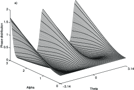
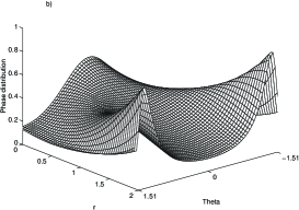
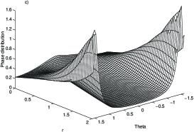
Figure 5.13: Phase distribution for TSYDS for a) $P(\theta,\alpha)$ for $r=0,\bar{n}=0$; b) $P(\theta,r)$ for $\bar{n}=0,\alpha=1$; c) $P(\theta,r)$ for $\bar{n}=2,\alpha=1$.

The phase distribution for superposition of quantum states, say even and/or odd coherent states, has two-peak structure [179]. For the present case we have displayed in Figs. 5.13a-c the phase distribution for TSYDS. In Fig. 5.13a we plotted the phase distribution for the Yurke-Stoler state with $r=0,$ and $\bar{n}=0$. In this figure we can see two-peak structure for even (odd) coherent state, which has been replaced by single peak at $\theta=0$ and two wings as $\theta\rightarrow\pm\pi$. This behaviour has been realized in studying the odd binomial states, see [180]. The squeezing effect in the Yurke-Stoler optical field in the cavity, i.e. squeezed Yurke-Stoler state ($\bar{n}=0$), has also been displayed in Fig. 5.13b. It is clear in our case that the bifurcation phenomenon appears in range of $\theta$ shorter than that for the squeezed state, where the central peak is at $\theta=0$ and the lateral peaks are at $\theta=\pm 1.5$. Finally we have plotted in Fig. 5.13c the effect of thermal noise in addition to squeezing for fixed value of the parameter $\alpha\quad(\alpha=2)$. From this figure we can realize that the latter bifurcation has been destroyed, e.g. the central peak is washed out, which indicates the influence of losses in the optical cavity, when the nonclassical effect disappeared.

5.2.6 Conclusions

In this section we have considered the thermal noise in the distribution of superposition squeezed and displaced number states. An observation of such a system can be found in a trapped ions, where a motion of a harmonically bound ${}^{9}Be^{+}$ ions can be used, see for example [35]. This can be seen when ions are initially cooled by a laser close to zero point of motion and the coupling between their motional and internal states due to applied (classical) radiation can be described by the Jaynes–Cummings-type interaction. In this case the evolution of the internal atomic state will create states having quantum character, such as number state. On the other hand, if the ions are not in the Fock state, the motional state is characterized by a density operator whose diagonal elements have a number distribution $P(n)$ given by

$$P_{\downarrow}(t)=\frac{1}{2}\left[1+{\sum_{n=0}^{\infty}P(n)\cos(2\Omega_{n,n+1}t)\exp(-\nu_{n}t)}\right],$$ (5.2.49)

where $P_{\downarrow}$ is the probability of occupation in $|\downarrow\rangle$ ($|\downarrow\rangle$ is the hyperfine ground state of the ion), $\Omega_{n,n+1}$ is the Rabi frequency and $\nu_{n}$ is the decoherence rate between levels $|n\rangle$ and $|n+1\rangle$. $P(n)$ in expression (5.2.49) has been derived analytically for more general case, see equation (5.2.26), which can be controlled by the detuning Doppler cooling. Therefore we have an advantage to measure and control further phenomena by using the photon-number distribution given by (5.2.49).

For thermal superposition of squeezed and displaced states, the nonclassical effects have been traced via quasiprobability distribution functions, second-order correlation function, photon-number distribution, and phase distribution. We have seen that the correlation between different oscillators is essentially responsible for nonclassical effects, which has been demonstrated by the behaviour of Wigner function and photon-number distribution. The thermal light photons have tendency to bunch each other, this has been reflected in the behaviour of our state, for example the normalized correlation function $g^{(2)}(0)$ shows sub-Poissonian statistics but only for real and negative values of $\epsilon$, provided $\bar{n}$ is sufficiently small. $Q$-function exhibits always two peaks strucure provided that $\epsilon\neq 0$. Nevertheless, for the sake of comparison, it is important to remind that for the state (5.1.1), as we have shown in section 5.1, the $W$-function exhibits negative values for a wide range of phase space, i.e. the role of the interference term is less effective; $g^{(2)}(0)$ shows sub-Poissonian statistics for a different type of $\epsilon$, i.e. $\epsilon=\pm 1,i$; further $Q$-function displays multi-peak structures related to the excitation number $n$.

We have also calculated the photon-number distribution using the Wigner function and we have shown that the oscillations in $P(n)$ are increased when the squeezing is considered for superposition of thermal coherent fields in the cavity. Also we have found that the purity coefficient for this superposition which is mixed rather than pure. Finally, we have considered the phase properties of the optical system and shown that for a short range of $\theta$, bifurcation distinguishing the squeezed states can occur in the absence of thermal noise. This phenomenon disappears with increasing thermal noise in the cavity.

5.3 Quantum statistics of a solvable three-boson squeeze operator model

In this section we introduce a highly correlated multidimensional squeeze operator. This operator consists of three modes in interaction and it represents the time-dependent evolution operator of the interaction part of the Hamiltonian [181, 182] determined as

$$\begin{array}[]{lc}\frac{H}{\hbar}=\sum_{j=1}^{3}\omega_{j}\hat{a}_{j}^{\dagger}\hat{a}_{j}-i\lambda_{1}\left\{\hat{a}_{1}\hat{a}_{2}\exp[i(\omega_{1}+\omega_{2})t]-{\rm h.c.}\right\}\\ \\ \hskip 72.26999pt-i\lambda_{2}\left\{\hat{a}_{1}\hat{a}_{3}\exp[i(\omega_{1}+\omega_{3})t]-\mbox{h.c.}\right\}-i\lambda_{3}\left\{\hat{a}_{2}\hat{a}_{3}^{\dagger}\exp[i(\omega_{2}-\omega_{3})t]-\mbox{h.c.}\right\},\end{array}$$ (5.3.4)

where $\hat{a}_{j}$ and $\hat{a}_{j}^{\dagger}$ satisfy the commutation relations

$$[\hat{a}_{k},\hat{a}_{j}^{\dagger}]=\delta_{kj},\quad\delta_{kj}=\{_{0\quad k\leavevmode\nobreak\ \neq j}^{1\quad k=j},$$ (5.3.5)

and $\omega_{j}$ are the field frequencies and $\lambda_{j}$ are the effective intermodal coupling constants. In fact, Hamiltonian equation (5.3.4) describes a two-photon parametric coupling of modes $1$ and $2$, and $1$ and $3$ (two photons are simultaneously created or annihilated in both the quantum modes through the interaction with classical pumping mode), and linear interaction of modes $2$ and $3$. By introducing the transformation $\hat{A}_{j}=\hat{a}_{j}\exp(i\omega_{j}t)$, the Hamiltonian (5.3.4) may be transformed into the interaction picture,

$$\frac{H}{\hbar}=-i\lambda_{1}(\hat{A}_{1}\hat{A}_{2}-\hat{A}_{1}^{\dagger}\hat{A}_{2}^{\dagger})-i\lambda_{2}(\hat{A}_{1}\hat{A}_{3}-\hat{A}_{1}^{\dagger}\hat{A}_{3}^{\dagger})-i\lambda_{3}(\hat{A}_{3}^{\dagger}\hat{A}_{2}-\hat{A}_{3}\hat{A}_{2}^{\dagger}).$$ (5.3.6)

It is important mentioning that the interaction (5.3.6) can be established in a bulk nonlinear crystal exhibiting the second-order nonlinear properties in which three dynamical modes of frequencies $\omega_{1},\omega_{2},\omega_{3}$ are induced by three beams from lasers of these frequencies. When pumping this crystal by means of the corresponding strong coherent pump beams, as indicated in the Hamiltonian, we can approximately fulfil the phase-matching conditions for the corresponding processes, in particular if the frequencies are close each other (biaxial crystals may be helpful in such an arrangement). Also a possible use of quasi-phase matching may help in the realization, which is, however, more difficult technologically [183]. Another possibility to realize such interaction is to use a nonlinear directional coupler which is composed of two optical waveguides fabricated from nonlinear material described by the quadratic susceptibility $\chi^{(2)}$. Modes 1 and 2 propagate in the first waveguide and 1 and 3 in the second waveguide (auxiliary device such as bandgap quantum coupler [129] or a set of mirrors can be used to generate two identical modes (mode 1) in each waveguide). The interactions between the modes in the same waveguide are established by strong pump coherent light. In this case the coupling constants $\lambda_{1}$ and $\lambda_{2}$ are proportional to the second order susceptibility $\chi^{(2)}$ of the medium and they also include the amplitudes of the pump. The linear coupling between modes 2 and 3 is established through the evanescent waves [96].

For completeness the time-evolution operator of equation (5.3.6) is

$$\exp(-i\frac{H}{\hbar}t)=\exp[\lambda_{1}t(\hat{A}^{\dagger}_{1}\hat{A}_{2}^{\dagger}-\hat{A}_{1}\hat{A}_{2})+\lambda_{2}t(\hat{A}_{1}^{\dagger}\hat{A}_{3}^{\dagger}-\hat{A}_{1}\hat{A}_{3})+\lambda_{3}t(\hat{A}_{3}\hat{A}_{2}^{\dagger}-\hat{A}_{3}^{\dagger}\hat{A}_{2})],$$ (5.3.7)

which can be identified well with a time-dependent three-mode squeeze operator

$$\hat{S}(\underline{r})=\exp[r_{1}(\hat{A}^{\dagger}_{1}\hat{A}_{2}^{\dagger}-\hat{A}_{1}\hat{A}_{2})+r_{2}(\hat{A}_{1}^{\dagger}\hat{A}_{3}^{\dagger}-\hat{A}_{1}\hat{A}_{3})+r_{3}(\hat{A}_{3}\hat{A}_{2}^{\dagger}-\hat{A}_{3}^{\dagger}\hat{A}_{2})],$$ (5.3.8)

where $r_{j}=\lambda_{j}t$, with $0\leq r_{j}<\infty$, $j=1,2,3$ and $\underline{r}=(r_{1},r_{2},r_{3})$. It is evident that this squeeze operator must involve two different squeezing mechanisms (terms involving $r_{1}$ and $r_{2}$) and then it is more complicated than squeezing operators that have appeared in the literature earlier [2, 7, 39]-[43]. Now if we set

$$\hat{A}=(\hat{A}_{1}^{\dagger}\hat{A}_{2}^{\dagger}-\hat{A}_{1}\hat{A}_{2}),\quad\hat{B}=(\hat{A}_{1}^{\dagger}\hat{A}_{3}^{\dagger}-\hat{A}_{1}\hat{A}_{3}),\quad\hat{C}=(\hat{A}_{2}\hat{A}_{3}^{\dagger}-\hat{A}_{3}\hat{A}_{2}^{\dagger}),$$ (5.3.9)

then we have the following commutation relations

$$[\hat{A},\hat{B}]=-\hat{C},\quad\quad[\hat{B},\hat{C}]=\hat{A},\quad\quad[\hat{C},\hat{A}]=\hat{B}.$$ (5.3.10)

We may conclude that the squeeze operator (5.3.8) involves correlations and can be regarded as the exponential of linear combination of three generators, which are closed under the commutation relations (5.3.10), and it represents the $su(1,1)$ generalized coherent state. As we mentioned earlier the quantum correlation between different quantum mechanical systems is responsible for the nonclassical effects for such type of operator.

Our plan of studying operator (5.3.8) will be as follows: We derive the basic relations for three-mode squeeze operator and then we discuss three-mode photon-number sum and photon-number difference as well as squeezing phenomenon. Moreover, we give two examples of three modes squeezed states related to this operator which are three-mode squeezed coherent and number states. For these two states we discuss sub-Poissonian phenomenon and quasidistribution functions.

5.3.1 Properties of the correlated quantum systems

Squeezed state of light is distinguishable by long-axis variance of noise ellipse for one of its quadratues in phase-space. This property is connected with the pairwise nature of the unitary operator (2.1.3) under which the initial state evolves. This operator exhibits some well-known basic relations summarized in the literature [2]. We introduce similar relations corresponding to the three-mode squeeze operator (5.3.8), and then we use them to deduce the three-mode photon-number sum and difference. Also we discuss squeezing phenomenon related to this operator.

The squeeze operator (5.3.8) provides a Bogoliubov transformation of the annihilation and creation operators that mixe the three modes as

$$\begin{array}[]{rl}\bar{A}_{1}\equiv\hat{S}^{-1}(\underline{r})\hat{A}_{1}\hat{S}(\underline{r})=\hat{A}_{1}f_{1}+\hat{A}_{2}^{\dagger}f_{2}+\hat{A}_{3}^{\dagger}f_{3},\\ \bar{A}_{2}\equiv\hat{S}^{-1}(\underline{r})\hat{A}_{2}\hat{S}(\underline{r})=\hat{A}_{2}g_{1}+\hat{A}_{3}g_{2}+\hat{A}_{1}^{\dagger}g_{3},\\ \bar{A}_{3}\equiv\hat{S}^{-1}(\underline{r})\hat{A}_{3}\hat{S}(\underline{r})=\hat{A}_{3}h_{1}+\hat{A}_{1}^{\dagger}h_{2}+\hat{A}_{2}h_{3},\end{array}$$ (5.3.14)

where

$$\begin{array}[]{lr}f_{1}=\cosh\mu+\frac{2r_{3}^{2}}{\mu^{2}}\sinh^{2}(\frac{\mu}{2}),\quad f_{2}=\frac{r_{1}}{\mu}\sinh\mu-\frac{2r_{2}r_{3}}{\mu^{2}}\sinh^{2}(\frac{\mu}{2}),\\ f_{3}=\frac{r_{2}}{\mu}\sinh\mu+\frac{2r_{1}r_{3}}{\mu^{2}}\sinh^{2}(\frac{\mu}{2}),\quad g_{1}=\cosh\mu-\frac{2r_{2}^{2}}{\mu^{2}}\sinh^{2}(\frac{\mu}{2}),\\ g_{2}=\frac{r_{3}}{\mu}\sinh\mu+\frac{2r_{1}r_{2}}{\mu^{2}}\sinh^{2}(\frac{\mu}{2}),\quad g_{3}=\frac{r_{1}}{\mu}\sinh\mu+\frac{2r_{2}r_{3}}{\mu^{2}}\sinh^{2}(\frac{\mu}{2}),\\ h_{1}=\cosh\mu-\frac{2r_{1}^{2}}{\mu^{2}}\sinh^{2}(\frac{\mu}{2}),\quad h_{2}=\frac{r_{2}}{\mu}\sinh\mu-\frac{2r_{1}r_{3}}{\mu^{2}}\sinh^{2}(\frac{\mu}{2}),\\ h_{3}=\frac{-r_{3}}{\mu}\sinh\mu+\frac{2r_{1}r_{2}}{\mu^{2}}\sinh^{2}(\frac{\mu}{2}),\end{array}$$ (5.3.20)

where $\mu=\sqrt{r_{1}^{2}+r_{2}^{2}-r_{3}^{2}}$ and $r_{3}^{2}<r_{1}^{2}+r_{2}^{2}$. The derivation of these relations is given in appendix B.

The commutation relations (5.3.5) under the transformations (5.3.14) hold also for the operators $\bar{A}_{j}$. Using these transformations we can easily calculate the statistical properties for each mode. It is worth to mention that the corresponding expressions for the single mode squeezed operator [2] and for two-mode squeezed operator [39] can be obtained from (5.3.14) by taking $r_{2}=r_{3}=0,$ and $\hat{A_{3}}\rightarrow\hat{0}$ together with $\hat{A_{2}}\rightarrow\hat{A}_{1}$ for only single mode case.

We may point out that a strong correlation is built up between the three modes described by squeeze operator (5.3.8). This is quite obvious for the case of the parametric amplification when two mode waves are mixed to generate a third wave via nonlinear medium, e.g. in an optical crystal with nonlinear second order susceptibility [2]. This can be demonstrated with the help of three-mode pure squeezed vacuum states $\hat{S}(\underline{r})\prod_{j=1}^{3}|0_{j}\rangle$, where $\hat{S}(\underline{r})$ is the squeeze operator (5.3.8). In this case the eigenstates of the three-mode photon-number difference $\hat{A}_{1}^{\dagger}\hat{A}_{1}-\hat{A}_{2}^{\dagger}\hat{A}_{2}-\hat{A}_{3}^{\dagger}\hat{A}_{3}$ correspond to zero eigenvalue, thus

$$\Delta(\hat{A}_{1}^{\dagger}\hat{A}_{1}-\hat{A}_{2}^{\dagger}\hat{A}_{2}-\hat{A}_{3}^{\dagger}\hat{A}_{3})^{2}=0.$$ (5.3.21)

However, the situation will be different for three-mode photon-number sum, using (5.3.14) and after minor calculations we obtain

$$\begin{array}[]{rl}\Delta(\hat{A}_{1}^{\dagger}\hat{A}_{1}+\hat{A}_{2}^{\dagger}\hat{A}_{2}+\hat{A}_{3}^{\dagger}\hat{A}_{3})^{2}=f^{2}_{1}(f^{2}_{1}-1)+g^{2}_{3}(1+g^{2}_{3})\\ +h^{2}_{2}(1+h^{2}_{2})+2(f^{2}_{1}g^{2}_{3}+f^{2}_{1}h^{2}_{2}+h^{2}_{2}g^{2}_{3}).\end{array}$$ (5.3.24)

In order to see the correlation between modes we have to calculate the fluctuations for both sum and difference operators thus having

$$\begin{array}[]{rl}2\left(\langle\hat{A}^{\dagger}_{1}\hat{A}_{1}\hat{A}^{\dagger}_{2}\hat{A}_{2}\rangle+\langle\hat{A}^{\dagger}_{1}\hat{A}_{1}\hat{A}^{\dagger}_{3}\hat{A}_{3}\rangle+\langle\hat{A}^{\dagger}_{2}\hat{A}_{2}\hat{A}^{\dagger}_{3}\hat{A}_{3}\rangle-\langle\hat{A}^{\dagger}_{1}\hat{A}_{1}\rangle\langle\hat{A}^{\dagger}_{2}\hat{A}_{2}\rangle\right.\\ -\left.\langle\hat{A}^{\dagger}_{1}\hat{A}_{1}\rangle\langle\hat{A}^{\dagger}_{3}\hat{A}_{3}\rangle-\langle\hat{A}^{\dagger}_{2}\hat{A}_{2}\rangle\langle\hat{A}^{\dagger}_{3}\hat{A}_{3}\rangle\right)=2(f^{2}_{1}g^{2}_{3}+f^{2}_{1}h^{2}_{2}+h^{2}_{2}g^{2}_{3}).\end{array}$$ (5.3.27)

It is clear that this quantity has non-zero value and this is the signature of photon-number correlation between modes.

Now we show how quantum correlations between the systems can give rise to squeezing if operators act in the spaces not only corresponding to three systems (three-mode squeezing) but also to two systems (two-mode squeezing), rather than to the individual systems (single-mode squeezing). This will be done using three-mode pure squeezed vacuum states $\hat{S}(\underline{r})\prod_{j=1}^{3}|0_{j}\rangle$ as before. For this purpose, using results of section 4.2, we calculate the squeezing variances for three-mode squeezing quadratures given by (4.2.4) and (4.2.5) in terms of three-mode pure squeezed vacuum states. After minor algebra we get

$$\begin{array}[]{rl}\langle(\triangle\hat{X})^{2}\rangle=\frac{1}{4}\Bigl{[}f^{2}_{1}+f^{2}_{2}+f^{2}_{3}+g^{2}_{1}+g^{2}_{2}+g^{2}_{3}\\ +h^{2}_{1}+h^{2}_{2}+h^{2}_{3}+4h_{2}g_{3}+4f_{1}h_{2}+4f_{1}g_{3}\Bigr{]},\end{array}$$ (5.3.30)

$$\begin{array}[]{rl}\langle(\triangle\hat{Y})^{2}\rangle=\frac{1}{4}\Bigl{[}f^{2}_{1}+f^{2}_{2}+f^{2}_{3}+g^{2}_{1}+g^{2}_{2}+g^{2}_{3}\\ +h^{2}_{1}+h^{2}_{2}+h^{2}_{3}+4h_{2}g_{3}-4f_{1}h_{2}-4f_{1}g_{3}\Bigr{]}.\end{array}$$ (5.3.33)

As we mentioned earlier the expressions for the single-mode and two-mode squeezing can be obtained easily from (5.3.30) and (5.3.33). It should be taken into account that $C=\frac{1}{2},1,\frac{3}{2}$ corresponding to the single-mode, two-mode and three-mode squeezing, respectively.

From (5.3.30) and (5.3.33) one can easily prove that the model cannot exhibit single-mode squeezing, e.g. for the first mode we have

$$S_{1}=S_{2}=2(f^{2}_{2}+f^{2}_{3}),$$ (5.3.34)

where the relations between the coefficients $f_{j}$ resulting from the commutation rules of $\hat{A}_{j}$ have been used to get such relation.

Figure 5.14: $S_{2}$ against squeeze parameter $r_{1}$ for three-mode squeezing and for $r_{3}=0.1$, $r_{2}=0.1$ (solid curve) and $0.2$ (short-dahed curves); and for two-mode squeezing (between modes 1 and 2, long-dashed curve) $(r_{2},r_{3})=(0.2,0.1)$.

For compound modes the system can provide two-mode (only between modes (1, 2) and (1,3)) as well as three-mode squeezing in the $Y$-quadrature as shown in Fig. 5.14 (for the shown values of squeeze parameters). From this figure one can observe that the behaviour of three-mode squeezing factors is smoothed in such a way that they are initially squeezed and their squeezing values reach their maximum, then they start again to decrease into unsqueezed values for large domain of $r_{1}$ (which is not shown in the figure). Also, the initial values of squeezing are sensitive to the values of the squeeze parameters (compare solid and short-dashed curves). Concerning two-mode squeezing factor (long-dashed curve) one can see it is monotonically decreasing function with lower limit $-1$. It is important mentioning that the squeeze operator under discussion cannot practically provide maximum squeezing (for three-mode squeezing), i.e. $S_{2}=-1$, and this, of course, is in contrast with the single-mode and two-mode squeeze operators (2.1.3) and (2.1.4) where they can display maximum squeezing for large values of squeeze parameter, however, they cannot provide squeezing initially. In conclusion it is quite obvious that squeezing can occur in the combined systems even if the individual systems are not themselves squeezed. The mechanism for this process is the correlation between the systems.

5.3.2 Three-mode squeezed coherent and number states

Here we examine the Glauber second-order correlation function for squeezed coherent states and squeezed number states related to the three-mode squeeze operator (5.3.8). Further we discuss the anticorrelation properties for three-mode squeezed coherent states.

First we define the three-mode squeezed coherent states as

$$|\underline{\alpha},\underline{r}\rangle\equiv\hat{S}(\underline{r})\hat{D}(\underline{\alpha})|0\rangle_{1}|0\rangle_{2}|0\rangle_{3},$$ (5.3.35)

where $\hat{S}(\underline{r})$ is the three-mode squeeze operator (5.3.8) and $\hat{D}(\underline{\alpha})$ is the three-mode Glauber displacement operator given by

$$\hat{D}(\underline{\alpha})=\exp\sum_{j=1}^{3}(\alpha_{j}\hat{A}_{j}^{\dagger}-\alpha_{j}^{*}\hat{A}_{j}),$$ (5.3.36)

and $\underline{\alpha}=(\alpha_{1},\alpha_{2},\alpha_{3})$.

The unitarity of the operator (5.3.8) provides that three-mode squeezed coherent states are not orthonormal but they are complete in the following sense

$$\hat{1}=\frac{1}{\pi^{3}}\int\int\int|\underline{\alpha},\underline{r}\rangle\langle\underline{r},\underline{\alpha}|d^{2}\alpha_{1}d^{2}\alpha_{2}d^{2}\alpha_{3}.$$ (5.3.37)

Using (5.3.14) the mean photon numbers for various modes in three-mode squeezed coherent states are given by

$$\begin{array}[]{rl}\langle\hat{n}_{1}\rangle_{\rm coh}=|f_{1}\alpha_{1}+f_{2}\alpha^{*}_{2}+f_{3}\alpha^{*}_{3}|^{2}+f^{2}_{2}+f^{2}_{3},\\ \langle\hat{n}_{2}\rangle_{\rm coh}=|g_{1}\alpha_{2}+g_{2}\alpha_{3}+g_{3}\alpha^{*}_{1}|^{2}+g^{2}_{3},\end{array}$$ (5.3.40)

and the photon-number variances are

$$\begin{array}[]{rl}\langle(\Delta\hat{n}_{1})^{2}\rangle_{\rm coh}=(2f_{1}^{2}-1)\langle\hat{n}_{1}\rangle_{\rm coh}-(f_{1}^{2}-1)^{2},\\ \langle(\Delta\hat{n}_{2})^{2}\rangle_{\rm coh}=(2g_{3}^{2}+1)\langle\hat{n}_{2}\rangle_{\rm coh}-g_{3}^{4},\end{array}$$ (5.3.43)

where ${\rm coh}$ stands for squeezed coherent states. Expressions related with the 3rd mode can be obtained from those of the 2nd mode by using the following transformation

$$(g_{1},g_{2},g_{3})\rightarrow(h_{3},h_{1},h_{2}).$$ (5.3.44)

Having obtained equations (5.3.40) and (5.3.43), we are ready to examine the second-order correlation function given by (4.1.1). In the following we restrict our discussions to the first mode $1$, because the other modes would have similar behaviour.

In phase space, squeezed coherent states $|\alpha,r\rangle$ are represented by a noise ellipse with the origin at $\alpha$, and they do not exhibit sub-Poisson distribution, i.e. they exhibit Poisson distribution at $r=0$ which is growing rapidly to superthermal distribution, i.e. $g^{(2)}(0)>2$, and it persists for a large domain of $r$ [70, 71]. In our model of three-mode squeezed coherent states we show that they exhibit only partial coherence behaviour, i.e. $1<g^{(2)}(0)<2$.

The condition for sub-Poissonian statistics is that the variance $\langle(\triangle\hat{n}_{j})^{2}\rangle$ must be less than the mean photon number $\langle\hat{n}_{j}\rangle$. We show that this condition will not be fulfilled for all modes, i.e. sub-Poissonian light cannot be obtained, because we have, e.g. for the first mode, the inequality

$$2|f_{1}^{2}\alpha_{1}+f_{2}\alpha^{*}_{2}+f_{3}\alpha^{*}_{3}|^{2}+f^{2}_{2}+f^{2}_{3}<0,$$ (5.3.45)

which will not be satisfied for any values of the coherent amplitudes $\alpha_{j}$.

For the first mode $\hat{A}_{1}$ we have

$$g_{1}^{(2)}(0)=1+\left[\frac{2(f_{1}^{2}-1)\langle\hat{n}_{1}\rangle_{coh}-(f_{1}^{2}-1)^{2}}{\langle\hat{n}_{1}\rangle^{2}_{\rm coh}}\right].$$ (5.3.46)

It is clear that when $r_{j}=0$, we recover the normalized second-order correlation function for coherent states. According to (5.3.46), to reach Poissonian statistics or thermal statistics, the expectation value $\langle\hat{n}_{1}\rangle$ of the photon number should have the following values:

$$\langle\hat{n}_{1}\rangle_{\rm p}=\frac{1}{2}(f_{1}^{2}-1),\qquad\langle\hat{n}_{1}\rangle_{\rm th}=f^{2}_{1}-1,$$ (5.3.47)

where subscripts ${\rm p}$ and ${\rm th}$ denote the corresponding quantities for Poisson and thermal distributions, respectively. For instance, to obtain thermal field, from (5.3.40) and (5.3.47), i.e. $\langle\hat{n}_{1}\rangle_{\rm th}$, we have

$$|f_{1}\alpha_{1}+f_{2}\alpha^{*}_{2}+f_{3}\alpha^{*}_{3}|^{2}=0.$$ (5.3.48)

It is clear that (5.3.48) is satisfied only when $\alpha_{j}=0$, i.e. for three-mode squeezed vacuum states, and hence super-thermal statistics cannot be obtained. Similar procedures show that Poissonian statistics cannot be obtained. This is a consequence of intermodal correlations of three-mode squeezed coherent states, for $\alpha_{j}\neq 0$, light exhibits only partially coherence. This can be seen in Fig. 5.15, where we display the normalized normal second-order correlation function for the first mode against $r_{1}$ for $\alpha_{j}=2\exp(i\frac{\pi}{4}),j=1,2,3$, $r_{3}=0.2$ with $r_{2}=0.4,0.8,$ and $1.5$ corresponding to solid, short-dashed, and long-dashed curves, respectively. Also we have displayed the corresponding normalized second-order correlation function for two-mode squeezed coherent state (centered curve) for the amplitudes $\alpha_{j}=2\exp(i\frac{\pi}{4}),j=1,2$, for sake of comparison. In this figure it is clear that partial coherence is dominant, and it persists for large values of $r_{1}$ and the initial values of $g_{j}^{(2)}(0)$ are sensitive to $r_{2}$. However, the normalized second-order correlation function for two-mode squeezed coherent state (centered curve) is a growing function, starting from 1 (Poisson distribution) when there is no squeezing $r_{1}=0$, and becomes stable for large values of $r$ displaying partial coherence behaviours. These values exceed those for three-mode squeezed coherent state for large domain of $r$.

Figure 5.15: Normalized normal second-order correlation function $g_{1}^{(2)}(0)$ (first mode) for three-mode squeezed coherent state against $r_{1}$, when $\alpha_{j}=2\exp(i\frac{\pi}{4}),j=1,2,3$, $r_{3}=0.2$, taking $r_{2}=0.4$ (solid curve), $0.8$ (short-dashed curve) and $1.5$ (long-dashed curve); centered curve is corresponding to the second-order correlation function for two-mode squeezed coherent state and $\alpha_{j}=2\exp(i\frac{\pi}{4}),j=1,2$.

Second, we discuss the sub-Poisson properties of three-mode squeezed number states. This state can be written with the aid of three-mode squeeze operator as

$$|\underline{n},\underline{r}\rangle\equiv\hat{S}(\underline{r})|n_{1}\rangle|n_{2}\rangle|n_{3}\rangle,$$ (5.3.49)

for simplicity we set $\underline{n}=(n_{1},n_{2},n_{3})$.

The mean photon numbers in three-mode squeezed number state are

$$\begin{array}[]{lr}\langle\hat{n}_{1}\rangle_{\rm n}=\bar{n}_{1}f^{2}_{1}+(\bar{n}_{2}+1)f^{2}_{2}+(\bar{n}_{3}+1)f^{2}_{3},\\ \langle\hat{n}_{2}\rangle_{\rm n}=\bar{n}_{2}g^{2}_{1}+\bar{n}_{3}g^{2}_{2}+(\bar{n}_{1}+1)g^{2}_{3},\end{array}$$ (5.3.52)

and the variances of the photon number are

$$\begin{array}[]{lr}\langle(\Delta\hat{n}_{1})^{2}\rangle_{\rm n}=f_{1}^{2}f_{2}^{2}[\bar{n}_{1}+\bar{n}_{2}+2\bar{n}_{1}\bar{n}_{2}+1]+f_{1}^{2}f_{3}^{2}[\bar{n}_{1}+\bar{n}_{3}+2\bar{n}_{1}\bar{n}_{3}+1]\\ +f_{2}^{2}f_{3}^{2}[\bar{n}_{2}+\bar{n}_{3}+2\bar{n}_{2}\bar{n}_{3}],\\ \\ \langle(\Delta\hat{n}_{2})^{2}\rangle_{\rm n}=g_{1}^{2}g_{2}^{2}[\bar{n}_{3}+\bar{n}_{2}+2\bar{n}_{2}\bar{n}_{3}]+g_{1}^{2}g_{3}^{2}[\bar{n}_{1}+\bar{n}_{2}+2\bar{n}_{1}\bar{n}_{2}]\\ +g_{2}^{2}g_{3}^{2}[\bar{n}_{1}+\bar{n}_{3}+2\bar{n}_{1}\bar{n}_{3}+1],\end{array}$$ (5.3.58)

where $\bar{n}_{j}$ is the mean photon number for the $j$th mode. The expression for the third mode can be obtained using (5.3.44). It is worthwhile to refer to [70, 71, 184, 73, 185], where further discussions related to squeezed number states are given. For instance, when the squeezing is not significant, i.e. $r$ is small, the normalized second-order correlation function can be less than unity, which indicates that the light field has sub-Poissonian statistics [71]. Furthermore, squeezed vacuum state exhibits super-Poisson statistics (precisely superthermal statistics) for $r\neq 0$ [24]. Here, in contrast to the latter results, we prove that three-mode squeezed number state can exhibit thermal statistics when $\bar{n}_{j}=0,j=1,2,3$, i.e. for three-mode squeezed vacuum states, otherwise sub-Poissonian statistics or partially coherence behaviour is dominant. We focus our attention to the first mode. According to the definition of normalized second-order correlation function to obtain thermal statistics, we need to have

$$\langle(\Delta\hat{n}_{1})^{2}\rangle_{\rm n}-\langle\hat{n}_{1}\rangle_{\rm n}-\langle\hat{n}_{1}\rangle^{2}_{\rm n}=0;$$ (5.3.59)

from (5.3.52) and (5.3.58) and after minor algebra one finds

$$\bar{n}_{1}(\bar{n}_{1}+1)f^{4}_{1}+\bar{n}_{2}(\bar{n}_{2}+1)f^{4}_{2}+\bar{n}_{3}(\bar{n}_{3}+1)f^{4}_{3}=0.$$ (5.3.60)

It is clear that the equality sign is only satisfied for $\bar{n}_{j}=0,j=1,2,3$. In other words, superthermal statistics will never occur. This is in contrast with the squeezed number state.

Figure 5.16: Normalized normal second-order correlation function for: a) three-mode squeezed number states against $r_{2}$ for different modes, when $\bar{n}_{j}=1,j=1,2,3$, $(r_{1},r_{3})=(0.5,0.3)$ for mode 1 (solid curve), mode 2 (short-dashed curve) and mode 3 (long-dashed curve); b) for single mode squeezed number states (solid curve, $\bar{n}_{1}=1$) and two-mode squeezed number state (dashed curve, $\bar{n}_{j}=1,j=1,2$) against squeezing parameter $r$.

In Fig. 5.16a we depict normalized second-order correlation function for single mode case for three-mode squeezed number state against $r_{2}$ for $\bar{n}_{j}=1,j=1,2,3$ and $(r_{1},r_{3})=(0.5,0.3)$. We notice in general that partially coherence behaviour is dominant again. Further we can see sub-Poissonian behaviour for small values of $\mu$ for modes 1 and 3 with maximum value at the third one. For sake of comparison, we displayed the normalized second-order correlation functions for single mode (dashed curve) and two-mode (solid curve) squeezed number states in Fig. 5.16b for $\bar{n}_{j}=1,j=1,2$, where we can see that both of them have sub-Poissonian statistics for lower values of squeeze parameter, otherwise they characterize partially coherence behaviour of light beams.

Finally we turn our attention to discuss the effect of intermodal correlations in terms of anticorrelations in three-mode squeezed coherent states. We do this by investigating the behaviour of the Cauchy-Schwarz inequality giving by (4.1.6). In doing so we have to derive the expectation values of cross photon-number operators between various modes, which are given in appendix C. In Fig. 5.17 we have plotted the quantity $I_{j,k}$ indicating the violation of Cauchy-Schwarz inequality between the $j$th mode and the $k$th mode against squeeze parameter $r_{1}$, where $(r_{2},r_{3})=(0.4,0.2)$ and $\alpha_{j}=1,j=1,2,3$ (real). Further, solid, short-dashed, and long-dashed curves correspond to the $I_{j,k}$ quantity obtained between $(1,2),(2,3),$ and $(1,3)$ modes, respectively. In general, photon antibunching can occur in dependence on the values of the parameters $r_{j}$ and $\alpha_{j}$. More precisely, in this figure we can observe that all curves can take on negative values reflecting the violation of the inequality, i.e. the photons are more strongly correlated than it is possible classically. The strongest violation of this inequality occurs in the $(1,3)$ mode for lower $r_{1}$ and then the curve monotonically increases to positive values for larger $r_{1}$. The weakest violation is in the $(2,3)$ mode for which the curve decreases from positive values to the negative values as $r_{1}$ increases. Clearly, the violation of this inequality is sensitive to the values of squeeze parameters and coherent amplitudes. As is known, the correspondence between quantum and classical theories can be established via Glauber-Sudarshan $P$-representation. But $P$-representation does not have all the properties of a classical distribution function, especially for quantum fields. So the violation of the Cauchy-Schwarz inequality provides explicit evidence of the quantum nature of intermodal correlation between modes which imply that the $P$-distribution function possesses strong quantum properties [150].

Figure 5.17: The quantity $I_{j,k}$, indicating the violation of the Cauchy-Schwarz inequality betwen the $j$th mode and $k$th mode, against squeeze parameter $r_{1}$, where $(r_{2},r_{3})=(0.4,0.2)$ and $\alpha_{j}=1,j=1,2,3$ (real). Solid, short-dashed, and long-dashed curve correspond to the above quantity considered for modes $(1,2),(2,3)$, and $(1,3)$, respectively.

5.3.3 Quasiprobability distribution functions

Here we extend our work to include the quasiprobability distribution functions. We consider such functions for three-mode squeezed coherent and number states. We give only one example in this thesis for the joint quasiprobability functions for three-mode squeezed coherent states since this type of functions carries information on the intermodal correlations between different modes in the quantum mechanical system. Results of section 4.3 should be used.

(a) Three-mode squeezed coherent states

Here we study quasiprobability distribution functions for three-mode squeezed coherent state, specified by the density matrix $\hat{\rho}_{\rm coh}=|\underline{\alpha},\underline{r}\rangle\langle\underline{r},\underline{\alpha}|$ and $|\underline{\alpha},\underline{r}\rangle$ is given by (5.3.35). Thus substituting $\hat{\rho}_{\rm coh}$ into (4.3.1) and using transformations (5.3.14) together with the Baker-Hausdorff identity for normal ordering of operators and after some minor calculations we have the $s$-parametrized joint characteristic function

$$\begin{array}[]{lr}C^{(3)}_{\rm coh}(\zeta_{1},\zeta_{2},\zeta_{3},s)=\exp[\frac{1}{2}\sum_{j=1}^{3}(s|\zeta_{j}|^{2}-|\eta_{j}|^{2})]\\ \times\exp[(\alpha_{1}^{*}\eta_{1}-\alpha_{1}\eta^{*}_{1})+(\alpha_{2}^{*}\eta_{2}-\alpha_{2}\eta_{2}^{*})+(\alpha_{3}^{*}\eta_{3}-\alpha_{3}\eta_{3}^{*})],\end{array}$$ (5.3.63)

where we have used the following abbreviations

$$\eta_{1}=\zeta_{1}f_{1}-\zeta_{2}^{*}g_{3}-\zeta_{3}^{*}h_{2},\quad\eta_{2}=\zeta_{2}g_{1}-\zeta_{1}^{*}f_{2}+\zeta_{3}h_{3},\quad\eta_{3}=\zeta_{3}h_{1}+\zeta_{2}g_{2}-\zeta_{1}^{*}f_{3}.$$ (5.3.64)

Having obtained the characteristic function, we are ready to find the $s$-parametrized quasiprobability functions for three-mode squeezed coherent state by inserting (5.3.63) into (4.3.2) and evaluating the integral by using the identity (A.4) in appendix A three times; the calculations are straightforward but rather lengthy, thus we get

$$\begin{array}[]{lr}W^{(3)}_{\rm coh}(\beta_{1},\beta_{2},\beta_{3},s)=\frac{2}{\pi^{3}}\frac{1}{\nu_{1}\nu_{2}(2f_{2}^{2}+2f^{2}_{3}+1-s)}\exp\left[-\frac{2|\beta_{1}|^{2}}{2f_{2}^{2}+2f^{2}_{3}+1-s}\right]\\ \\ \qquad\times\exp\left\{\frac{1}{4\nu_{1}}\left[(A^{2}-C^{2})\cos^{2}\phi+(B^{2}-D^{2})\sin^{2}\phi+(CD-AB)\sin(2\phi)\right]\right\}\\ \\ \qquad\times\exp\left\{\frac{1}{4\nu_{2}}\left[(B^{2}-D^{2})\cos^{2}\phi+(A^{2}-C^{2})\sin^{2}\phi-(CD-AB)\sin(2\phi)\right]\right\},\end{array}$$ (5.3.70)

where

$$\nu_{1}=\mu_{1}\cos^{2}\phi+\mu_{2}\sin^{2}\phi+\mu_{3}\sin(2\phi),\quad\nu_{2}=\mu_{2}\cos^{2}\phi+\mu_{1}\sin^{2}\phi-\mu_{3}\sin(2\phi);\quad$$ (5.3.71)

here

$$\begin{array}[]{lr}\mu_{1}=\frac{1}{2}(2f_{2}^{2}+2f^{2}_{3}+1-s)^{-1}\left[2f_{1}^{2}(1-s)-2g_{3}^{2}(1+s)-(1-s^{2})\right],\\ \mu_{2}=\frac{1}{2}(2f_{2}^{2}+2f_{3}^{2}+1-s)^{-1}\left[2f_{1}^{2}(1-s)-2h_{2}^{2}(1+s)-(1-s^{2})\right],\\ \mu_{3}=(2f_{2}^{2}+2f_{3}^{2}+1-s)^{-1}\left[2f_{1}^{2}g_{2}h_{1}+g_{1}h_{3}(1+s)\right].\end{array}$$ (5.3.75)

In equation (5.3.70) we have also used the following definitions

$$\begin{array}[]{lr}A=(\tilde{\alpha_{2}^{*}}-\tilde{\alpha_{2}})+2f_{1}g_{3}(2f_{2}^{2}+2f_{3}^{2}+1-s)^{-1}(\tilde{\alpha_{1}^{*}}-\tilde{\alpha_{1}}),\\ B=(\tilde{\alpha_{3}^{*}}-\tilde{\alpha_{3}})+2f_{1}h_{2}(2f_{2}^{2}+2f_{3}^{2}+1-s)^{-1}(\tilde{\alpha_{1}^{*}}-\tilde{\alpha_{1}}),\\ C=(\tilde{\alpha_{2}^{*}}+\tilde{\alpha_{2}})-2f_{1}g_{3}(2f_{2}^{2}+2f_{3}^{2}+1-s)^{-1}(\tilde{\alpha_{1}^{*}}+\tilde{\alpha_{1}}),\\ D=(\tilde{\alpha_{3}^{*}}+\tilde{\alpha_{3}})-2f_{1}h_{2}(2f_{2}^{2}+2f_{3}^{2}+1-s)^{-1}(\tilde{\alpha_{1}^{*}}+\tilde{\alpha_{1}}),\end{array}$$ (5.3.80)

where $\phi=\frac{1}{2}\tan^{-1}\left(\frac{2\mu_{3}}{\mu_{1}-\mu_{2}}\right)$, $\tilde{\alpha_{j}}=(\bar{\alpha}_{j}-\beta_{j})$, $j=1,2,3$ and $\bar{\alpha_{j}}$ represents the expectation value of the operators $\bar{A_{j}}$ given by equation (5.3.14) in terms of the coherent state. The three-mode functions $W^{(3)}_{\rm coh}(\beta_{1},\beta_{2},\beta_{3},s)$ given in (5.3.70) are 6-dimensional Gaussian functions and display the nonclassical correlation nature by involving the terms $A^{2},B^{2},$ etc. when the cross-terms $\beta_{1}\beta_{2},\beta_{1}\beta_{3}$, etc. are not zero. Furthermore, we can see that the three-mode $P$ representation does not exist at least for some values of squeezing parameters $r_{j}$, i.e. if $\nu_{1}=0$ or $\nu_{2}=0$ or both (see equation (5.3.70)), the physical reason for non-conditional breaking down of the $P$-function lies in the extremely strong correlation between the amplitudes of the three modes of the system during the evolution determined by squeeze operator [5]. Such tightly correlation causes that the modes may no longer fluctuate independently even in small amount such as allowed in a pure coherent states [39].

Now we turn our attention to single mode case, using similar procedure as before. The $s$-parametrized quasiprobability function takes the form

$$W^{(1)}_{\rm coh}(\beta_{j},s)=\frac{2}{\pi(\tau_{j}-s)}\exp\left(-2\frac{|\beta_{j}-\bar{\alpha}_{j}|^{2}}{\tau_{j}-s}\right),$$ (5.3.81)

where $j=1,2,3$ and

$$\tau_{1}=2f^{2}_{2}+2f^{2}_{3}+1,\quad\tau_{2}=2g^{2}_{3}+1,\quad\tau_{3}=2h^{2}_{2}+1.$$ (5.3.82)

Light fields for which the $P$-representation is not a well-behaved distribution will exhibit nonclassical features. Clearly single mode $P$-function is well defined, because the parametric systems evolution broadens $P$-distribution (increases the radius of the Wigner contour compared to the initial one) [39] and reflects that there is no (single mode) nonclassical behaviour, e.g. sub-Poissonian statistics and squeezing. Furthermore, it has been shown that $P$-function for the superposition of two fields is the convolution of the $P$-function for each field considered individually [139], so that (5.3.81) (with $s=1$) describes the superposition of $P$-function of a coherent state with complex amplitude $\bar{\alpha}_{j}$ and $P$-function of a chaotic mixture with variance $\frac{1}{2}(\tau_{j}-1)$ [5], i.e. displaced thermal light. Further, equation (5.3.81) has a Gaussian form in phase space with width and center dependent on $r_{j},\alpha_{j}$ and with a circular symmetric contour as a result of the fact that two quadrature variances are equal. Consequently the single mode photon-number distribution does not exhibit oscillations, in contrast with this for squeezed coherent state [168], owing to the noise ellipse of $W$-function which is isotropic.

Now we investigate single mode phase distribution in terms of $Q$-function, i.e. $s=-1$. Using the same procedures as in section 5.2.5 we arrive at

$$\begin{array}[]{lr}P(\theta)=\frac{1}{2\pi\sqrt{(\tau_{j}+1)}}\exp\left[\frac{b_{j}^{2}-4|\bar{\alpha}_{j}|^{2}}{2(\tau_{j}+1)}\right]\Bigl{\{}\sqrt{(\tau_{j}+1)}\exp\left[-\frac{b_{j}^{2}}{2(\tau_{j}+1)}\right]\\ +\frac{b_{j}\sqrt{\pi}}{2}\left[1+{\rm erf}(\frac{\sqrt{2}b_{j}}{\sqrt{\tau_{j}+1}})\right]\Bigr{\}},\end{array}$$ (5.3.85)

where

$$b_{j}=\bar{\alpha}_{j}\exp(-i\theta)+\bar{\alpha}^{*}_{j}\exp(i\theta),$$ (5.3.86)

with $j=1,2,3$, $\bar{\alpha}_{j}$ have the same meaning as before, and ${\rm erf(.)}$ is the Gauss error function (5.2.38).

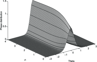
Figure 5.18: Phase distribution $P(\theta,r_{1})$ against $\theta$ and $r_{1}$ for the first mode as output from three-mode squeezed coherent state for $\alpha_{j}=1,j=1,2,3,r_{2}=1$ and $r_{3}=0.5$.

Here we restrict our investigation to real $\alpha_{j}$, i.e. $b_{j}=2\bar{\alpha}_{j}\cos\theta$, detailed examination to the formula (5.3.85) shows that it is a $2\pi$-periodic function, a symmetric function ($P(-\theta)=P(\theta)$) around $\theta=0$ and also it has its maximum height at $\theta=0$. Moreover, this formula has a similar structure as that for coherent states (which can be recovered from (5.3.85) by setting $r_{j}=0$). This means that the phase distribution of the single mode exhibits a one-peak structure for all values of $\alpha_{j}$ and $r_{j}$ (see Fig. 5.18 for shown values of parameters). That is the phase distribution of the single-mode as output from three-mode squeezed coherent state is insensitive to the quantum correlations between the systems. This situation is the same as that of two-mode squeezed coherent state, i.e. when $r_{2}=r_{3}=0$ [61]. However, it has been shown that the joint phase distribution for the two-mode squeezed vacuum depends only on the sum of the phases of the two modes, and that the sum of the two phases is locked to a certain value as the squeezing parameter increases [61, 62].

(b) Three-mode squeezed number state

Here we calculate single mode $s$-parametrized characteristic and quasiprobability functions for mode 1, for three-mode squeezed number state (5.3.49). Therefore $s$-parametrized single mode characteristic function can be written as follows

$$C_{\rm sn}^{(1)}(\zeta_{1},,s)=\exp[\frac{1}{2}|\zeta_{1}|^{2}(s-2f^{2}_{2}-2f^{2}_{3})]L_{n_{1}}(|\zeta_{1}|^{2}f^{2}_{1})L_{n_{2}}(|\zeta_{1}|^{2}f^{2}_{2})L_{n_{3}}(|\zeta_{1}|^{2}f^{2}_{3}),$$ (5.3.87)

where (5.1.6) has been used, $L_{k}(.)$ are the Laguerre polynomials of order $k$, and subscript ${\rm sn}$ stands for three-mode squeezed number states.

The single mode $s$-parametrized quasiprobability function for mode 1 is given by Fourier transformation of (5.3.87) as

$$W_{\rm sn}^{(1)}(\beta_{1},s)=\frac{2}{\pi(\tau_{1}-s)}\prod_{j=1}^{3}L_{n_{j}}[f_{j}^{2}\frac{\partial^{2}}{\partial\beta_{1}\partial(-\beta_{1}^{*})}]\exp\left[-\frac{2|\beta_{1}|^{2}}{\tau_{1}-s}\right],$$ (5.3.88)

where $\tau_{1}$ is given in (5.3.82). In derivation of (5.3.88) we used differentiation under the sign of integral to perform the integration and the identity (A.4) in appendix A. Expressions for the second mode and third mode can be obtained from (5.3.88) by replacing functions $f_{j}$ by functions $g_{j}$ and $h_{j}$.

Figure 5.19: $W$-function for the single mode (mode 1) as output from three-mode squeezed number state, assuming the first mode is $|1\rangle$ and the other modes are in vacuum for $(r_{1},r_{2},r_{3})=(0.8,0.9,0.6)$.

Here we discuss the behaviour of $W$-function for the first mode when it is in the Fock state $|1\rangle$ while the other modes are in vacuum. In fact, $W$-function of squeezed Fock state $|1\rangle$ is well characterized by inverted hole which is stretched as a consequence of squeezing parameter [71]. In the following we can use $L_{1}(x)=1-x$ to analyze the behaviour of the model under discussion. For this case it is clear that, from equation (5.3.88), $W$-function can exhibit negative values only inside the circle $|\beta_{1}|^{2}<\frac{2f_{1}^{2}-1}{4f_{1}^{2}}$ with center at the origin. However, the maximum value will be established at the circle $|\beta_{1}|^{2}=\frac{4f_{1}^{4}-1}{4f_{1}^{2}}$. Hence, $W$-function will not exhibit stretching since the variables ${\rm Re}\beta_{1}$ and ${\rm Im}\beta_{1}$ are not involving squeezing factor which plays an essential role for stretched quadratures of squeezed number state. As a result the radii of these circles are dependent on squeeze parameters $r_{j}$, so the negative values of $W$-function will be sensitive to the values of squeeze parameters, i.e. the function has negative values for a range of $|\beta_{1}|$ shorter than for individual Fock state $|1\rangle$, where it exhibits negative values inside the circle $|\beta_{1}|^{2}<\frac{1}{2}$. This can be recognized if one compares the well known shape of $W$-function of Fock state $|1\rangle$ with that of the single-mode case as output from three-mode squeezed number states. For this purpose Fig. 5.19 is displayed for $W$-function of $|1,0,0\rangle$ against $x={\rm Re}\beta_{1}$ and $y={\rm Im}\beta_{1}$ for $(r_{1},r_{2},r_{3})=(0.8,0.9,0.6)$. We can see that the well known negative values of $W$-function of Fock state $|1\rangle$ are smoothed out, in turn, the circle of negative values is enlarged, as we have shown earlier.

The phase distribution for the $j$th mode, which is in Fock state $|n_{j}\rangle$ while the other modes are in vacuum states, evolves under the action of three-mode squeezed operator (5.3.8), with the aid of $Q$-function, to

$$P(\theta_{j})=\frac{1}{2\pi},$$ (5.3.89)

which is uniform distribution. In other words, in spite of the system is highly correlated the phase distribution in the single mode of purely nonclassical state is phase insensitive. This agrees with the fact that the states are represented by a density matrix which is diagonal in the number state basis, having random phase distribution [58].

5.3.4 Conclusions

In this section we have introduced new type of multidimensional squeeze operator which is more general than usually used and which includes two different squeezing mechanisms. This operator arises from the time-dependent evolution operator for the Hamiltonian representing mutual interaction between three different modes of the field. The origin of the nonclassical effects of this operator model is the correlation between the systems where we have shown that the quadratures squeezing can occur in the combination systems rather than in the individual systems.

The quantum statistical properties corresponding to this operator have been traced by means of the variances of the photon-number sum and difference, squeezing phenomenon, Glauber second-order correlation function, violation of Cauchy-Schwarz inequality, quasiprobability distribution functions and phase probability distribution, considered for three-mode coherent and number states.

For three-mode squeezed coherent state, we found that the second-order correlation function describes partially coherent field provided that one mechanism of squeezing is always surviving, which can be demonstrated also by means of quasiprobability distribution function in single modes. Nevertheless, this behaviour is in contrast with behaviour of squeezed coherent states, where second-order correlation function can display superthermal statistics, i.e. $g^{(2)}(0)>2$. We have found strong violation for Cauchy-Schwarz inequality in some modes, i.e. the photons are more strongly correlated than it is allowed classically. Concerning the single-mode phase distribution, single peak structure is dominant for all values of parameters provided that coherent amplitudes are real. The signature of the correlations between the three modes appears straightforwardly in the form of quasiprobability functions.

For three-mode squeezed number states, the second-order correlation function is in agreement with that for the squeezed number state and in general it exhibits partial coherence; however, sub-Poissonian behaviour is attained for small values of $\mu$ and the maximum value is obtained only for $r_{j}=0,j=1,2,3$. Nevertheless, it cannot exhibits superthermal statistics. Also the range of negative values of the $W$-function, for a single mode, are highly sensitive to squeeze parameters. Phase distribution, for a single mode, is insensitive to correlation between modes, and it displays a uniform form.

Chapter 6 Scientific results and their analysis: part II (dynamic regime)

In this part we investigate the quantum properties of some dynamical systems in the framework of interaction of radiation modes with nonlinear media described nonlinear couplers. We have considered three types of such models when two, three or four modes are evolved within. In general, all of these models are composed from two waveguides of the length $L$ through which the interacting modes evolve. The interaction between the different modes in the same waveguide can be established by strong laser pumping, however, the interaction between the two waveguides occurs by means of evanescent waves. Instead of initial coherent states at the input beams, the Fock states generated for instance in a micromaser can be introduced. Outgoing fields are detected as single or compound modes by means of homodyne, photocounting or coincidence detection. Further, the values of the coupling constants between the different modes in the device are chosen for the reason of simple calculations and illustration of the physical behaviour of the system. We mainly demonstrate the effect of their mutual relations and their magnitudes are not substantial for such demonstrations. For an experimental realization these values can be estimated as $(10^{11}-10^{12})s^{-1}$, provided that the pumping laser of power in mW is used, producing about $10^{19}$ photons/s, which is sufficient power to neglect quantum noise in pumping beams. Then all the effects shown are interpreted on the corresponding reduced time scale. Initial state amplitudes or photon numbers are chosen in units because switching properties are examined on the quantum level of single photons.

In the following section we investigate the quantum properties of the first model which includes two-mode case.

6.1 Quantum statistics and dynamics of nonlinear couplers with nonlinear exchange

In this section we discuss the quantum statistical properties of nonlinear couplers composed of two waveguides operating by the second subharmonic generation assuming strong coherent pumping and linear exchange of energy between waveguides by means of evanescent waves, however we additionally take into account the influence of nonlinear coupling of the parametric type of both the waveguides. This system is suggested to be described by the following Hamiltonian:

$$\begin{array}[]{lr}\frac{\hat{H}}{\hbar}=\sum_{j=1}^{2}\left\{\omega_{j}\hat{a}_{j}^{\dagger}\hat{a}_{j}+\lambda_{j}\left[\hat{a}_{j}^{\dagger 2}\exp(i\mu_{j}t)+{\rm h.c.}\right]\right\}\\ \\ +\lambda_{3}\left\{\hat{a}_{1}\hat{a}_{2}^{\dagger}\exp[i\phi_{1}(t)]+{\rm h.c.}\right\}+\lambda_{4}\left\{\hat{a}_{1}\hat{a_{2}}\exp[-i\phi_{2}(t)]+{\rm h.c.}\right\},\end{array}$$ (6.1.4)

where $\hat{a}_{1}(\hat{a}_{1}^{\dagger})$, $\hat{a}_{2}(\hat{a}_{2}^{\dagger}$) are annihilation (creation) operators of the fundamental modes in the first and second waveguides having frequencies $\omega_{1}$ and $\omega_{2}$, respectively, $\mu_{j}$ are related with the frequency of the second-harmonic modes described classically as strong coherent fields, $\phi_{j}(t)$, $j=1,2$, are related to the difference- and sum-frequencies of modes $1$ and $2$, respectively, $\lambda_{1}$ and $\lambda_{2}$ are nonlinear coupling constants for the second subharmonic generation in the first and second waveguides, respectively, $\lambda_{3}$ is the coupling constant for linear exchange between waveguides through evanescent waves, $\lambda_{4}$ is the coupling constant for the nonlinear exchange through simultaneous annihilation or creation of a photon in both the subharmonic modes on expense of pumping and h.c. means the Hermitian conjugate terms (for further details concerning the optical parametric processes, see [88] (Chap. 10)).

When $\mu_{j}=0$ and only the degenerate term is considered, we have the well-known Hamiltonian, in the interaction picture, for squeezed light generation [7], where $\lambda_{1}$ (or $\lambda_{2}$) represents the coupling constant proportional to the quadratic susceptibility of the second-order nonlinear process (degenerate parametric down-conversion with classical coherent pumping), or the coupling constant proportional to the cubic susceptibility of the third-order nonlinear process (degenerate four-wave mixing with classical coherent pumping) [186]. If additionally $\phi_{1}(t)=\phi_{2}(t)=0$, the Hamiltonian (6.1.4) represents a mixture of second subharmonic generation, frequency conversion and parametric amplification in the interaction picture [5, 87, 100]. Schematically, this Hamiltonian is represented in Fig. 6.1.

Figure 6.1: Scheme of quantum nonlinear coupler with linear and nonlinear coupling formed from two nonlinear waveguides described by the quadratic susceptibility $\chi^{(2)}$. The beams are described by the photon annihilation operators as indicated; $z=vt$ is the interaction length. Both the waveguides are pumped by strong classical coherent waves. Outgoing fields are examined as single or compound modes by means of homodyne detection to observe squeezing of vacuum fluctuations, or by means a set of photodetectors to measure photon antibunchibng and sub-Poissonian photon statistics in the standard ways.

Solution of the equations of motion in the Heisenberg picture for the Hamiltonian (6.1.4) are

$$\begin{array}[]{lr}\hat{a}_{1}(t)\exp(-it\frac{\mu_{1}}{2})=\hat{a}_{1}(0)K_{1}(t)+\hat{a}_{1}^{\dagger}(0)L_{1}(t)+\hat{a}_{2}(0)M_{1}(t)+\hat{a}_{2}^{\dagger}(0)N_{1}(t),\\ \\ \hat{a}_{2}(t)\exp(-it\frac{\mu_{2}}{2})=\hat{a}_{2}(0)K_{2}(t)+\hat{a}_{2}^{\dagger}(0)L_{2}(t)+\hat{a}_{1}(0)M_{2}(t)+\hat{a}_{1}^{\dagger}(0)N_{2}(t),\end{array}$$ (6.1.8)

where the explicit forms of the time dependent coefficients, which contain all the features of the structure, and the details about the solution are given in appendix D.

One can see from this solution (see appendix D) that when $\bar{\Omega}_{1}$ and $\bar{\Omega}_{2}$ are real, the coupler switches the energy between the modes which propagate inside since the solution will include trigonometric functions [5]. Nevertheless, if $\bar{\Omega}_{1}$ and $\bar{\Omega}_{2}$ are pure imaginary, the Heisenberg solutions provide hyperbolic functions, which are growing rapidly with time, and the coupler operates as amplifier for the input modes [187]. So that the behaviour of the coupler will be indicated essentially by the relation between coupling constants.

In what follows, we shall employ the results obtained here to treat the squeezing phenomenon and quasiprobability distribution functions for the model under consideration.

6.1.1 Squeezing phenomenon

Here we study single-mode squeezing phenomenon when the modes are initially prepared in thermal states with the average thermal photon numbers $\bar{n}_{j},\quad j=1,2$ as well as in the coherent states. For this purpose (using results of section 4.2 and considering $\mu_{j}(t)$ to be the phase of the local oscillator in the relations (4.2.4) and (4.2.5), without loss of generality, we can cancel the high frequency terms, and $j=1,2$ stands for mode 1 and mode 2, respectively) we calculate the quantities $S_{j}(t)$ and $Q_{j}(t)$ which are defined in (4.9) for the initial thermal light. For the first mode we have the following expressions

$$\begin{array}[]{lr}S_{1}(t)=2\bar{n}_{1}[|L_{1}(t)|^{2}+|K_{1}(t)|^{2}]+2\bar{n}_{2}[|N_{1}(t)|^{2}+|M_{1}(t)|^{2}]+2|L_{1}(t)|^{2}+2|N_{1}(t)|^{2}\\ \\ +2(2\bar{n}_{1}+1)[L_{1}(t)K_{1}(t)+{\rm c.c.}]+2(2\bar{n}_{2}+1)[M_{1}(t)N_{1}(t)+{\rm c.c.}],\end{array}$$ (6.1.12)

$$\begin{array}[]{lr}Q_{1}(t)=2\bar{n}_{1}[|L_{1}(t)|^{2}+|K_{1}(t)|^{2}]+2\bar{n}_{2}[|N_{1}(t)|^{2}+|M_{1}(t)|^{2}]+2|L_{1}(t)|^{2}+2|N_{1}(t)|^{2}\\ \\ -2(2\bar{n}_{1}+1)[L_{1}(t)K_{1}(t)+{\rm c.c.}]-2(2\bar{n}_{2}+1)[M_{1}(t)N_{1}(t)+{\rm c.c.}],\end{array}$$ (6.1.16)

where c.c. means the complex conjugate terms. The corresponding expressions for the second mode can be obtained from (6.1.12) and (6.1.16) by using the interchange $1\leftrightarrow 2$. Further, the other expressions related to the injected coherent light in the coupler are the same as (6.1.12) and (6.1.16), but setting $\bar{n}_{j}=0$.

It is known that the nonlinear coupler is a source of optical fields, the statistical properties of which are changed as a result of the linear and nonlinear interaction inside and between waveguides. Consequently, one can obtain nonclassical light from one input and, in addition, it can be switched.

Figure 6.2: Squeezing phenomenon for mode 1 when the modes are initially in coherent light and: a) for the first component $S_{1}(t)$; b) for the second component $Q_{1}(t)$; $\lambda_{3}=1$ for all curves; curves A, B and C are corresponding to $\lambda_{1}=\lambda_{2}=\lambda_{4}=0.25$, $\lambda_{1}=\lambda_{2}=\lambda_{4}=0.2$ and $\lambda_{1}=0.17$, $\lambda_{2}=\lambda_{4}=0.2$, respectively; straight line has been put to show the bound of squeezing.

We have plotted $S_{1}(t),Q_{1}(t)$ in Figs. 6.2a,b and $S_{2}(t),Q_{2}(t)$ in Figs. 6.3a,b, when the initial light is coherent, for different values of $\lambda_{k}$. Further we have chosen $\lambda_{3}=1$ for all curves and for the curve $A:\lambda_{1}=\lambda_{2}=\lambda_{4}=0.25$; for the curve $B:\lambda_{1}=\lambda_{2}=\lambda_{4}=0.20$, and for the curve $C:\lambda_{1}=0.17,\lambda_{2}=\lambda_{4}=0.2$. On the other hand, Fig. 6.4 gives $S_{1}(t)$ (first mode) when the initial light is thermal light with coupling constants as those for the curve C, where $\bar{n}_{1}=0.5$ and $\bar{n}_{2}=0.5$ (solid curve), 1.5 (dashed curve); straight line shows the bound of squeezing of the curves. Firstly, we start our discussion by studying the case of input coherent light. From these figures we can see how the coherent states, which are minimum-uncertainty states, evolve in the coupler to produce squeezed light. We can observe the oscillatory behaviour in these curves, showing that squeezing can be switched from one waveguide to the other in the course of time during power transfer. Moreover, squeezing can be interchanged between the two quadratures of the same waveguide. More precisely, for mode 1, squeezing can occur for all selected values of $\lambda_{k}$ in $S_{1}(t)$, but in $Q_{1}(t)$ only curves A, B can exhibit squeezing, as shown in Figs. 6.2a,b, which reflects the dependence of nonclassical behaviour on the strength of subharmonic generation.

Figure 6.3: Squeezing phenomenon for mode 2: a) for the first component $S_{2}(t)$; b) for the second component $Q_{2}(t)$; the values of the parameters $\lambda_{k}$ are as in Fig. 6.2.

For mode 2, we can see squeezing in all curves in both the quadratures, as shown in Figs. 6.3a,b. It can be easily seen that the amount of squeezing is sensitive to the strength of coupling $\lambda_{k}$ and that in general its values in the second component are more pronounced than those in the first one. Now if we turn our attention to the case of injected thermal light (Fig. 6.4c), we can observe that squeezing is available in the large interaction time. Further, $S_{1}(t)$ exhibits oscillatory behaviour and it evolves from unsqueezed values in the short range of interaction time, owing to the fact that thermal states are not minimum-uncertainty states, into squeezed values and eventually unsqueezed values can be recovered. Indeed, we proved numerically that this behaviour is periodically recovered with the time. Moreover, by comparing the dashed curve with the solid one, we can see that increasing of the photon number in the second waveguide causes decreasing of the amount of squeezing in the first one. This is related with the effect of evanescent waves between waveguides and shows how one can control light by light in the coupler. Finally, we can conclude that by controlling the input average thermal photon number and the interaction time (or the length of the coupler), the interaction under consideration can generate squeezed thermal light. It is worthwhile to refere to [70, 71, 73, 74], where more discussions related to squeezed thermal states are given.

Figure 6.4: Squeezing phenomenon for mode 1 when the modes are initially in thermal light for the first component $S_{1}(t)$ with $\bar{n}_{1}=0.5$, $\bar{n}_{2}=0.5$ (solid curve), $1.5$ (dashed curve) and the coupling constants $\lambda_{j}$ are the same as those for the curve C in Fig. 6.2.

6.1.2 Quasiprobability functions

Here we shall continue in our investigation for the statistical properties of the system under discussion in the basis of quasiprobability distribution functions for single-mode case only when both the modes are initially in number and coherent states.

(a) Input Fock states

The density operator for two-mode number states is

$$\hat{\rho}_{\rm n}(0)={\rm|n\rangle_{1}|m\rangle_{2}}{\rm{}_{2}\langle m|_{1}\langle n|},$$ (6.1.17)

where the subscript $n$ stands for Fock states case. The single-mode s-parametrized characteristic function for the first mode can be obtained using the results of section 4.3 together with the identity (5.1.6) as

$$C^{(1)}_{n,m}(\zeta,s,t)=\exp\left\{\frac{s}{2}|\zeta|^{2}-\frac{1}{2}[|\nu_{1}(t)|^{2}+|\nu_{2}(t)|^{2}]\right\}L_{n}(|\nu_{1}(t)|^{2})L_{m}(|\nu_{2}(t)|^{2}),$$ (6.1.18)

where

$$\nu_{1}(t)=\zeta K_{1}^{*}(t)-\zeta^{*}L_{1}(t),\quad\nu_{2}(t)=\zeta M_{1}^{*}(t)-\zeta^{*}N_{1}(t),$$ (6.1.19)

and $L_{m}(.)$ is the Laguerre polynomial of order $m$. Inserting (6.1.18) into (4.3.4), carrying out the integration numerically (the exact form can be found, see [189]) and taking $s=0$ we obtain the W-function. The result has been plotted in

Figure 6.5: W-function for the single mode (mode 1) for different values of time $t$ when both the modes are initially in the number states; the first mode is in the state $|1\rangle$ and the second mode is in the state $|0\rangle$ and $\lambda_{3}=1$, $\lambda_{1}=\lambda_{2}=\lambda_{4}=0.25$: a) for $t=\pi/100$; b) for $t=\pi/2$; c) for $t=\pi$.

Figs. 6.5 against $x={\rm Re}\beta_{1}$ and $y={\rm Im}\beta_{1}$, when the first state is the Fock state $|1\rangle$ and the second one is the vacuum state $|0\rangle$, i.e. $n=1,m=0$; $\lambda_{3}=1,\lambda_{1}=\lambda_{2}=\lambda_{4}=0.25$ and for shown values of time. In Fig. 6.5a we have the W-function for $t=\frac{\pi}{100}$, i.e. after short time interaction between the two modes we observe similar behaviour as for the W-function of the state $|1\rangle$, which means that pronounced negative values are exhibited. This behaviour of the W-function is completely different by increasing the time ($t=\frac{\pi}{2}$); we see disappearance of negative values of the quasidistribution and a stretched positive peak occurs (Fig. 6.5b). This form of $W$-function is close to that of squeezed vacuum states [7], i.e. squeezed vacuum states can be generated, in principle, in this model. It should be borne in mind that the specific direction of stretching for the quasiprobability function of squeezed states may be achieved by choosing a suitable value for the phase of squeeze parameter. Of course, in Fig. 6.5b, there is a negligible spike at the top of the peak which can be smoothed out by governing the coupler parameters. After larger time interaction $t=\pi$, the negative values are reached again, but they are less pronounced and asymmetry can be observed due to stretching (Fig. 6.5c). So we meet a time development of the W-function as a result of the power transfer between the two modes inside the coupler. This shows that the nonlinear directional coupler can be used as a source of quantum states. Further, we have found that the behaviour of the Q-function is consistent with that of $W$-function for the same shown values [189].

(b) Input coherent light

In a similar way as we followed in the case (a) we can study the same quantities when both the modes are initially in coherent states $|\alpha_{1},\alpha_{2}\rangle$. For the single-mode case the $s$-parametrized characteristic function and the $s$-parametrized quasiprobability function are given, respectively, as

$$\begin{array}[]{lr}C^{(1)}_{{\rm coh}}(\zeta,s,t)=\exp\left\{-\frac{1}{2}[1-s+2|L_{1}(t)|^{2}+2|N_{1}(t)|^{2}]|\zeta|^{2}+\zeta\bar{\alpha}_{1}^{*}(t)-\zeta^{*}\bar{\alpha}_{1}(t)\right\}\\ \\ \times\exp\left\{\frac{1}{2}\zeta^{2}[N^{*}_{1}(t)M^{*}_{1}(t)+L^{*}_{1}(t)K^{*}_{1}(t)]\right\}\\ \\ \times\exp\left\{\frac{1}{2}\zeta^{*2}[N_{1}(t)M_{1}(t)+L_{1}(t)K_{1}(t)]\right\},\end{array}$$ (6.1.25)

$$\begin{array}[]{lr}W^{(1)}_{{\rm coh}}(\beta,s,t)=\frac{1}{\pi\sqrt{[\frac{1-s}{2}+|L_{1}(t)|^{2}+|N_{1}(t)|^{2}]^{2}-|B_{1}(t)|^{2}}}\\ \\ \times\exp\left\{-\frac{[\frac{1-s}{2}+|L_{1}(t)|^{2}+|N_{1}(t)|^{2}]|\bar{\alpha}_{1}(t)-\beta|^{2}}{[\frac{1-s}{2}+|L_{1}(t)|^{2}+|N_{1}(t)|^{2}]^{2}-|B_{1}(t)|^{2}}\right\}\\ \\ \times\exp\left\{-\frac{\frac{1}{2}|B_{1}(t)|[E_{1}^{2}(t)+E_{1}^{*2}(t)]}{[\frac{1-s}{2}+|L_{1}(t)|^{2}+|N_{1}(t)|^{2}]^{2}-|B_{1}(t)|^{2}}\right\},\end{array}$$ (6.1.31)

where

$$\begin{array}[]{lr}B_{1}(t)=N^{*}_{1}(t)M^{*}_{1}(t)+L^{*}_{1}(t)K^{*}_{1}(t)=|B_{1}(t)|\exp[2i\delta_{1}(t)],\\ E_{1}(t)=[\bar{\alpha}_{1}(t)-\beta]\exp[i\delta_{1}(t)],\end{array}$$ (6.1.34)

and $\bar{\alpha}_{1}(t)$ is the average of the first mode operator $\hat{A}_{1}(t)$ with respect to input coherent light.

From (6.1.31), the $P$-function is not well defined as an ordinary function for $|L_{1}(t)|^{2}+|N_{1}(t)|^{2}<|B_{1}(t)|$ and hence the nonclassical effects such as squeezing of vacuum fluctuations can occur, as we have seen before.

Figure 6.6: W-function for the single mode (mode 1) for different values of time $t$ when both the modes are initially in the coherent states; $|\alpha_{1}|^{2}=|\alpha_{2}|^{2}=2$ and $\lambda_{k}$ are the same as in Fig. 6.6: a) for $t=\pi$; b) for $t=2\pi$.

Furthermore, the nonclassical effect, especially squeezing of vacuum fluctuations in the case of our system, can be recognized in the behaviour of $W$-function (and/or $Q$-function) in phase space as shown in Fig. 6.6 for shown values of parameters. For $t=0$, i.e. when there is no interaction between the two modes, the W-function is identical with that shown for a single mode representing a symmetric Gaussian bell in phase space. As soon as the interaction switches on ($t>0$), we observe that the Gaussian centre is shifted and the rotationally symmetric function of the initial state at $t=0$ gets to be squeezed in various phase space directions in dependence on time, as demonstrated in Figs. 6.6a,b. In other words, the initial symmetric contour of the $W$-function has been stretched as the interaction switches on, i.e. noise ellipse characterizing squeezed light appears, which rotates in the phase space as the interaction time progresses.

6.1.3 Conclusions

In this section we have examined the quantum statistical properties of radiation generated and propagated in the nonlinear optical coupler composed of two nonlinear waveguides operating by the second subharmonic processes, coupled linearly by evanescent waves and nonlinearly by nondegenerate optical parametric process. We have demonstrated regimes for generation and propagation of nonclassical light exhibited by squeeezing of vacuum fluctuations. We have also obtained quasidistribution functions for the initial light beams which are in Fock and coherent states. Compared to earlier results for nonlinear optical couplers we have shown that the nonlinear coupling increases in general quantum noise in the device even if in some cases it can support generation of nonclassical light.

The motivation for examination of the system under consideration arises from the previous investigations of the nonlinear couplers as promising devices to produce nonclassical light. When coherent light is injected initially in the system, squeezed as well as sub-Poissonian light can be generated [189] (the latter has not been analyzed here). For injected number states, squeezed vacuum states are produced. When thermal light initially enters the coupler, the coupler can operate as a microwave Josephson-junction parametric amplifier [63]. These effects have been recognized to result from the competition between linear and nonlinear properties of the system and are dependent on the initial amplitudes of the input fields. The crucial role plays here the mechanism of the energy exchange between waveguids.

6.2 Generation of squeezed light in a nonlinear asymmetric directional coupler

In this section we study the properties of three modes interacting in a nonlinear asymmetric directional coupler composed of a linear waveguide and a nonlinear waveguide operating by nondegenerate parametric amplification. We show that such a device is a source of single-mode squeezed light. This fact has been demonstrated, under certain conditions and for specific modes, for incident coherent beams in terms of the quasiprobability functions, photon-number distribution and phase distribution.

6.2.1 Equations of motion

We consider a device (nonlinear asymmetric directional coupler) as outlined in Fig. 6.7. It can be described by the Hamiltonian

$$\begin{array}[]{lr}\frac{\hat{H}}{\hbar}=[\sum_{j=1}^{3}\omega_{j}\hat{a}^{\dagger}_{j}\hat{a}_{j}]+i\lambda_{1}\left\{\hat{a}_{1}\hat{a}_{2}\exp[i(\omega_{1}+\omega_{2})t]-{\rm h.c.}\right\}\\ \\ +i\lambda_{2}\left\{\hat{a}_{1}\hat{a}^{\dagger}_{3}\exp[i(\omega_{1}-\omega_{3})t]-{\rm h.c.}\right\}+i\lambda_{3}\left\{\hat{a}_{2}\hat{a}^{\dagger}_{3}\exp[i(\omega_{2}-\omega_{3})t]-{\rm h.c.}\right\},\end{array}$$ (6.2.4)

where $\hat{a}_{j}(\hat{a}^{\dagger}_{j}),\quad j=1,2,3$ are the annihilation (creation) operators designated to the signal, idler and linear modes, respectively, $\lambda_{1}$ and $\lambda_{j},\quad j=2,3$ are the corresponding nonlinear and linear coupling constants; $\omega_{j}$ are the natural frequencies of oscillations of the uncoupled modes and h.c. is the Hermitian conjugate. The linear exchange between the two waveguides establishes through evanescent waves provided that $\omega_{1}\simeq\omega_{2}\simeq\omega_{3}$.

The dynamics of the system is described by the Heisenberg equations of motion which, using the slowly varying forms ($\hat{a}_{j}=\hat{A}_{j}\exp(-i\omega_{j}t),\quad j=1,2,3$), read

$$\begin{array}[]{lr}\frac{d\hat{A}_{1}}{dt}=-\lambda_{1}\hat{A}_{2}^{\dagger}-\lambda_{2}\hat{A}_{3},\\ \\ \frac{d\hat{A}_{2}}{dt}=-\lambda_{1}\hat{A}_{1}^{\dagger}-\lambda_{3}\hat{A}_{3},\\ \\ \frac{d\hat{A}_{3}}{dt}=\lambda_{2}\hat{A}_{1}+\lambda_{3}\hat{A}_{2}.\end{array}$$ (6.2.10)

These are three equations with their Hermitian conjugates forming a closed system which can be easily solved, restricting ourselves to the case $\lambda_{2}=\lambda_{3}=\frac{\lambda_{1}}{\sqrt{2}}$, to avoid the complexity in the calculations; this means that we consider stronger nonlinearity in the first waveguide compared with the linear exchange between waveguides, thereby having the solution

$$\begin{array}[]{lr}\hat{A}_{1}(t)=\hat{a}_{1}(0)f_{1}(t)+\hat{a}^{\dagger}_{1}(0)f_{2}(t)-\hat{a}_{2}(0)f_{3}(t)\\ -\hat{a}_{2}^{\dagger}(0)f_{4}(t)-\hat{a}_{3}(0)f_{5}(t)-\hat{a}^{\dagger}_{3}(0)f_{6}(t),\\ \\ \hat{A}_{2}(t)=\hat{a}_{2}(0)g_{1}(t)+\hat{a}^{\dagger}_{2}(0)g_{2}(t)-\hat{a}_{1}(0)g_{3}(t)\\ -\hat{a}_{1}^{\dagger}(0)g_{4}(t)-\hat{a}_{3}(0)g_{5}(t)-\hat{a}^{\dagger}_{3}(0)g_{6}(t),\\ \\ \hat{A}_{3}(t)=\hat{a}_{3}(0)h_{1}(t)+\hat{a}^{\dagger}_{3}(0)h_{2}(t)+\hat{a}_{2}(0)h_{3}(t)\\ +\hat{a}_{2}^{\dagger}(0)h_{4}(t)+\hat{a}_{1}(0)h_{5}(t)+\hat{a}^{\dagger}_{1}(0)h_{6}(t),\end{array}$$ (6.2.19)

where the time-dependent coefficients, i.e. $f_{j}(t),g_{j}(t),h_{j}(t)$, including all information about the system, are

Figure 6.7: Scheme of realization of interaction in (6.2.4) using a nonlinear asymmetric directional coupler which is composed of two optical waveguides fabricated from first-order ($\chi^{(1)}$) and second-order ($\chi^{(2)}$) materials, where $\chi$ designate susceptibility. Signal mode 1 and idler mode 2 propagate in the first waveguide and linear mode 3 in the second waveguide. The interaction between the signal and idler modes is established by strong pump coherent light, which is not indicated in figure, with the coupling constant $\lambda_{1}$. The interactions between the linear mode and the signal and idler are established linearly with the coupling constants $\lambda_{2}$ and $\lambda_{3}$, respectively.

$$\begin{array}[]{lr}f_{1,3}(t)=\frac{1}{2}\left[\cosh(\lambda_{1}t)\pm\cosh(\frac{\lambda_{1}t}{2})\cos(\bar{k}t)\pm\frac{1}{\sqrt{3}}\sinh(\frac{\lambda_{1}t}{2})\sin(\bar{k}t)\right],\\ \\ f_{2,4}(t)=\frac{1}{2}\left[\sinh(\lambda_{1}t)\mp\sinh(\frac{\lambda_{1}}{2}t)\cos(\bar{k}t)\mp\frac{1}{\sqrt{3}}\cosh(\frac{\lambda_{1}t}{2})\sin(\bar{k}t)\right],\\ \\ f_{5}(t)=\sqrt{\frac{2}{3}}\cosh(\frac{\lambda_{1}t}{2})\sin(\bar{k}t),\quad f_{6}(t)=-\sqrt{\frac{2}{3}}\sinh(\frac{\lambda_{1}t}{2})\sin(\bar{k}t),\\ \\ h_{1}(t)=\cosh(\frac{\lambda_{1}t}{2})\cos(\bar{k}t)-\frac{1}{\sqrt{3}}\sinh(\frac{\lambda_{1}t}{2})\sin(\bar{k}t),\\ \\ h_{2}(t)=-\sinh(\frac{\lambda_{1}t}{2})\cos(\bar{k}t)+\frac{1}{\sqrt{3}}\cosh(\frac{\lambda_{1}t}{2})\sin(\bar{k}t),\\ \\ h_{3,5}(t)=\sqrt{\frac{2}{3}}\cosh(\frac{\lambda_{1}t}{2})\sin(\bar{k}t),\quad h_{4,6}(t)=-\sqrt{\frac{2}{3}}\sinh(\frac{\lambda_{1}t}{2})\sin(\bar{k}t),\end{array}$$ (6.2.31)

where $\bar{k}=\frac{\sqrt{3}}{2}\lambda_{1}$ and the expressions for $g_{j}(t)$ are the same as those of $f_{j}(t)$.

In fact, the nature of the solution can show how the coupler does work. To be more specific, the time-dependent coefficients contain both trigonometric and hyperbolic functions. Consequently, the propagating beams inside the coupler can be amplified as well as switched between waveguides, i.e. between modes, in the course of time.

On the basis of the well known commutation rules for boson operators, the following relations can be proved for the time-dependent coefficients

$$\begin{array}[]{lr}f^{2}_{1}(t)-f^{2}_{2}(t)+f^{2}_{3}(t)-f^{2}_{4}(t)+f^{2}_{5}(t)-f^{2}_{6}(t)=1,\quad f_{1}(t)g_{4}(t)-f_{2}(t)g_{3}(t)\\ \\ +f_{3}(t)g_{2}(t)-f_{4}(t)g_{1}(t)-f_{5}(t)g_{6}(t)+f_{6}(t)g_{5}(t)=0,\\ \\ f_{1}(t)g_{3}(t)-f_{2}(t)g_{4}(t)+f_{3}(t)g_{1}(t)-f_{4}(t)g_{2}(t)-f_{5}(t)g_{5}(t)+f_{6}(t)g_{6}(t)=0.\end{array}$$ (6.2.37)

The remaining relations can be obtained from (6.2.37) by means of the following transformations

$$\begin{array}[]{lr}\Bigl{(}f_{1}(t),f_{2}(t),f_{3}(t),f_{4}(t),f_{5}(t),f_{6}(t)\Bigr{)}\\ \longleftrightarrow\Bigl{(}-g_{3}(t),-g_{4}(t),-g_{1}(t),-g_{2}(t),g_{5}(t),g_{6}(t)\Bigr{)}\\ \longleftrightarrow\Bigl{(}h_{5}(t),h_{6}(t),-h_{3}(t),-h_{4}(t),-h_{1}(t),-h_{2}(t)\Bigr{)}.\end{array}$$ (6.2.41)

Based on these results, we can study the quantum properties of the evolution of different modes in the model when they are initially prepared in coherent states. This will be demonstrated in the following parts by means of quasiprobability functions.

6.2.2 Quasiprobability functions

In the following we consider phase space distributions for the single-mode when all modes are initially prepared in coherent states $|\alpha_{1},\alpha_{2},\alpha_{3}\rangle$ before entering the coupler. We start from knowledge of the single-mode $s$-parametrized characteristic function which is suitable to describe the quantum statistics of light and for the first mode it takes the form

$$C_{1}(\zeta,s,t)=\exp\left\{\frac{1}{2}|\zeta|^{2}[s-|\eta_{1}(t)|]+|\eta_{2}(t)|(\zeta^{2}+\zeta^{*2})+[\bar{\alpha}_{1}^{*}(t)\zeta-\bar{\alpha}_{1}(t)\zeta^{*}]\right\},$$ (6.2.42)

where $\eta_{j}(t),\quad j=1,2$, are given by

$$\begin{array}[]{lr}\eta_{1}(t)=f^{2}_{1}(t)+f^{2}_{2}(t)+f^{2}_{3}(t)+f^{2}_{4}(t)+f^{2}_{5}(t)+f^{2}_{6}(t),\\ \\ \eta_{2}(t)=f_{1}(t)f_{2}(t)+f_{3}(t)f_{4}(t)+f_{5}(t)f_{6}(t).\end{array}$$ (6.2.46)

Now the $s$-parametrized single-mode quasiprobability functions of the signal mode, which can be derived in a similar way as we did in the previous section, are

$$\begin{array}[]{lr}W_{1}(\beta,s,t)=\frac{2}{\pi\sqrt{[A_{+}(t)-s][A_{-}(t)-s]}}\\ \\ \times\exp\left\{\frac{[l_{1}(t)-l^{*}_{1}(t)]^{2}}{2[A_{-}(t)-s]}-\frac{[l_{1}(t)+l^{*}_{1}(t)]^{2}}{2[A_{+}(t)-s]}\right\},\end{array}$$ (6.2.50)

where $l_{1}(t)=\bar{\alpha}_{1}(t)-\beta$ ($\bar{\alpha}_{1}(t)$ has the same meaning as before) and

$$A_{\pm}(t)=[f_{1}(t)\pm f_{2}(t)]^{2}+[f_{3}(t)\pm f_{4}(t)]^{2}+[f_{5}(t)\pm f_{6}(t)]^{2};$$ (6.2.51)

the other expressions for the idler and linear modes can be obtained from (6.2.42) and (6.2.50) by making use of the transformations (6.2.41); we except here the case $s=1$, which will be discussed shortly. Now let us start our investigation by demonstrating the behaviour of the $W$-function, i.e. setting $s=0$ in (6.2.50). In the language of mechanical analogy of a harmonic oscillator with dynamical conjugate variables $x$ and $y$, i.e $\beta=x+iy$, the $W$-function can be written in the form

$$W_{1}(x,y,t)=\frac{1}{2\pi\sqrt{\langle(\triangle\hat{X}(t))^{2}\rangle\langle(\triangle\hat{Y}(t))^{2}\rangle}}\exp\left\{-\frac{[x-\bar{\alpha}_{x}(t)]^{2}}{2\langle(\triangle\hat{X}(t))^{2}\rangle}-\frac{[y-\bar{\alpha}_{y}(t)]^{2}}{2\langle(\triangle\hat{Y}(t))^{2}\rangle}\right\},$$ (6.2.52)

where

$$\langle(\triangle\hat{X}(t))^{2}\rangle=\frac{A_{+}(t)}{4},\quad\quad\quad\langle(\triangle\hat{Y}(t))^{2}\rangle=\frac{A_{-}(t)}{4},$$ (6.2.53)

and $\bar{\alpha}_{1}(t)=\bar{\alpha}_{x}(t)+i\bar{\alpha}_{y}(t)$; $\langle(\triangle\hat{X}(t))^{2}\rangle$ and $\langle(\triangle\hat{Y}(t))^{2}\rangle$ are single-mode $x$- and $y$-quadrature variances, respectively.

Now from (6.2.52) and (6.2.53) together with (6.2.31) one can easily prove that the quadrature variances of the linear mode (single-mode squeezing) are

$$\langle(\triangle\hat{X}(t))^{2}\rangle=\frac{1}{4}\left\{\frac{4}{3}\sin^{2}(\bar{k}t)+[\cos(\bar{k}t)+\frac{1}{\sqrt{3}}\sin(\bar{k}t)]^{2}\right\}\exp(-\lambda_{1}t),$$ (6.2.54)

$$\langle(\triangle\hat{Y}(t))^{2}\rangle=\frac{1}{4}\left\{\frac{4}{3}\sin^{2}(\bar{k}t)+[\cos(\bar{k}t)-\frac{1}{\sqrt{3}}\sin(\bar{k}t)]^{2}\right\}\exp(\lambda_{1}t),$$ (6.2.55)

where $\bar{k}$ has the same meaning as before. Thus squeezing can be achieved in the linear waveguide in the $X$-quadrature. Moreover, it is clear that squeezing values become more pronounced for a large interaction time, i.e. for long length of the coupler $L$. This behaviour shows that changing the power of the linear interaction it is possible to transfer nonclassical properties, which are generated in the nonlinear waveguide, to the linear signal mode. For completeness, the uncertainty relation reads

$$\langle(\triangle\hat{X}(t))^{2}\rangle\langle(\triangle\hat{Y}(t))^{2}\rangle=\frac{1}{16}[1+\frac{16}{9}\sin^{4}(\bar{k}t)].$$ (6.2.56)

This formula reveals that the minimum-uncertainty relation holds only when $t=t_{s}=\frac{2m\pi}{\sqrt{3}\lambda_{1}}$ where $m$ is positive integer and we call $t_{s}$ a squeeze time. In this case the device provides the squeezed coherent light in the linear mode with squeeze parameter $r=\frac{2m\pi}{\sqrt{3}}$. It is important to mention that at $t=t_{s}$ the two waveguides become completely independent (cf. equations (6.2.31)) and the signal and idler modes can display perfect two-mode squeezing, which one can easily check with the help of two-mode quadrature variances. This can be explained as follows: A portion of the energy always remains within the guide into which the field was initially injected. This energy grows in the course of time until $t=t_{s}$, when the two guides are completely independent and hence the modes are trapped in their own guides. So that the linear mode can yield the well known single-mode squeezed light in the linear waveguide having its origin in the nonlinear waveguide in which the nonlinearity produces two-mode squeezing. For later times $t\neq t_{s}$, the device generates single-mode squeezed light in the linear waveguide where the corresponding $W$-function may be broader than that of the idealized squeezed coherent states [7]. This situation is close to that of a two-photon absorber (a two-photon absorption by a reservoir of two-level atoms from a single mode of the electromagnetic field [190]) where a squeezed state, which is not a minimum-uncertainty state, has been generated [191]. The origin of squeezing of initially unsqueezed light interacting with two-photon absorbers is that the squeezing is generated by simple quantum superposition of states of light [190].

We proceed in our discussion by focusing our attention on the $P$-function. We have shown earlier that this system is able to provide squeezed light and this should be reflected in the behaviour of the $P$-representation, i.e. setting $s=1$ in (6.2.50). The significant example for this situation is the behaviour of the linear mode. For this case, we can show that the single-mode quadrature squeezing is established provided that $A_{+}(t)-1<0$ and $A_{-}(t)-1>0$. It is evident that the $P$-function is not well-behaved function in this case and this is the indication of the nonclassical fields. Indeed, if we look at the model under consideration of a competition of parametric processes, we can find that this result is in contrast to the results in the literature for simpler systems of interacting modes starting from coherent states [5, 39, 40, 43, 181], where the delta function of the initial $P$-representation of coherent light for a single mode becomes well-behaved distribution during the interaction.

In the following we use the phase space distribution functions to study the photon-number distribution and phase distribution for the system under discussion.

6.2.3 Photon-number distribution

Photon-number distribution, i.e. the probability of finding $n_{1}$ photons in the signal mode at time $t$, can be obtained in the photodetection process, and can be determined by means of the relation (4.3.8) as

$$\begin{array}[]{lr}P(n_{1},t)=\frac{2}{\sqrt{[A_{+}(t)+1][A_{-}(t)+1]}}\exp\left\{\frac{[\bar{\alpha}_{1}(t)-\bar{\alpha}^{*}_{1}(t)]^{2}}{2[A_{-}(t)+1]}-\frac{[\bar{\alpha}_{1}(t)+\bar{\alpha}^{*}_{1}(t)]^{2}}{2[A_{+}(t)+1]}\right\}\\ \\ \times\sum^{n_{1}}_{r=0}\left[\frac{A_{+}(t)-1}{A_{+}(t)+1}\right]^{r}\left[\frac{A_{-}(t)-1}{A_{-}(t)+1}\right]^{n_{1}-r}\\ \\ \times{\rm L}^{-\frac{1}{2}}_{r}\left[-\frac{(\bar{\alpha}_{1}(t)+\bar{\alpha}^{*}_{1}(t))^{2}}{(1+A_{+}(t))(A_{+}(t)-1)}\right]{\rm L}^{-\frac{1}{2}}_{n_{1}-r}\left[\frac{(\bar{\alpha}_{1}(t)-\bar{\alpha}^{*}_{1}(t))^{2}}{(1+A_{-}(t))(A_{-}(t)-1)}\right],\end{array}$$ (6.2.62)

where $L^{\nu}_{n_{1}}(.)$ is the associated Laguerre polynomial and the integration has been carried out using the same technique as in appendix A.

It is convenient to compare this distribution with the corresponding Poisson distribution

$$P(n_{1},t)=\frac{\langle\hat{n}_{1}(t)\rangle^{n_{1}}}{n_{1}!}\exp[-\langle\hat{n}_{1}(t)\rangle],$$ (6.2.63)

which corresponds to fully coherent field with the same mean photon number $\langle\hat{n}_{1}(t)\rangle$. The expressions for the idler and linear modes should be obtained from (6.2.62) using the transformations (6.2.41).

Figure 6.8: Photon-number distribution $P(n_{1})$ for the signal mode for $\alpha_{j}=3\exp(i\frac{\pi}{3}),j=1,2,3,\quad t=1.5$ and $\lambda_{1}=0.3$. The dashed curve is the Poisson photon-number distribution.

In Fig. 6.8, we have plotted $P(n_{1},t=1.5)$ against $n_{1}$ for the signal mode (solid curve) for $\alpha_{j}=3\exp(i\frac{\pi}{3})$ and $\lambda_{1}=0.3$. For the sake of comparison, the corresponding photon distribution for coherent field, (6.2.63), is shown by dashed curve. For all numerical calculations $\sum_{n_{1}=0}^{\infty}P(n_{1},t)=1$ with good accuracy. We noted for the signal mode that the photon-number distribution exhibits always one-peak structure. From this figure we see that the behaviour is rather super-Poissonian as a result of quantum fluctuations because the solid curve is always broader than the corresponding dashed curve. So that, in general the Poissonian light evolves in the nonlinear waveguide as super-Poissonian light. On the other hand, we have realized earlier from the behaviour of $W$-function that squeezed states can be generated. However, these states are exhibiting oscillating photon-number distribution for certain values of squeeze parameter.

Figure 6.9: Photon-number distribution $P(n_{3})$ for the linear mode when $\alpha_{j}=0.5\exp(i\frac{\pi}{3}),j=1,2,3;\lambda_{1}=1$ and a) $t=t_{s}$ ; b) $t=5$.

Indeed, these oscillations can be recognized for the linear mode where this mode can display squeezed light (see Fig. 6.9, for shown values of parameters). From this figure we see the macroscopic oscillations of the photon-number distribution for squeezed light. Further, comparison of Figs. 6.9a and 6.9b shows that the nonclassical oscillations of $P(n_{3})$ are faster and more pronounced when $t$ increases. It is worthwhile mentioning that the case of Fig. 6.9a corresponds to squeezed light with squeeze parameter $r\simeq 3.6$.

In fact, the behaviour of the photon-number distribution in this device is slightly different from that of the nonlinear asymmetric coupler with strong classical stimulating light in the second harmonic mode [120] where oscillatory behaviour as well as sub-Poissonian statistics for specific modes in both linear and nonlinear waveguide are exhibited.

6.2.4 Phase distribution

We make use of the single-mode $Q$-function to investigate the phase distribution for the system under discussion using (4.20). The result of the integration has the form

$$\begin{array}[]{lr}P(\theta,t)=\frac{1}{\pi C(t)\sqrt{A_{+}(t)A_{-}(t)}}\exp\left\{\frac{[\bar{\alpha}_{1}(t)-\bar{\alpha}^{*}_{1}(t)]^{2}}{2[A_{-}(t)+1]}-\frac{[\bar{\alpha}_{1}(t)+\bar{\alpha}^{*}_{1}(t)]^{2}}{2[A_{+}(t)+1]}\right\}\\ \\ \times\left\{1+\frac{B(t)}{2}\sqrt{\frac{\pi}{C(t)}}\exp[\frac{B(t)^{2}}{4C(t)}][1+{\rm erf}(\frac{B(t)}{2\sqrt{C(t)}})]\right\},\end{array}$$ (6.2.67)

where

$$\begin{array}[]{lr}C(t)=\frac{2}{A_{-}(t)A_{+}(t)}[A_{+}(t)\sin^{2}\theta+A_{-}(t)\cos^{2}\theta],\\ B(t)=\frac{2}{A_{-}(t)A_{+}(t)}\left[A_{-}(t)\left(\bar{\alpha}_{1}(t)+\bar{\alpha}^{*}_{1}(t)\right)\sin\theta-iA_{+}(t)\left(\bar{\alpha}_{1}(t)-\bar{\alpha}^{*}_{1}(t)\right)\cos\theta\right],\end{array}$$ (6.2.70)

and ${\rm erf}(.)$ is the Gauss error function; $A_{\pm}(t)=4\langle(\triangle\hat{X}_{\pm}(t))^{2}\rangle$ with $\langle(\triangle\hat{X}(t))^{2}\rangle$ and $\langle(\triangle\hat{Y}(t))^{2}\rangle$ are single-mode $x$- and $y$-quadrature variances, respectively; $\bar{\alpha}_{1}(t)$ is the expectation value of the signal mode operator in coherent state.

Figure 6.10: Phase distribution $P(\theta,t)$ for the signal mode against $\theta$ and $t$ for $\lambda_{1}=0.6$ and a) $\alpha_{j}=0$; b) $\alpha_{j}=1,\quad j=1,2,3$.

The behaviour of this distribution in this device can be understood on the basis of the competition between the two-peak structure for the vacuum states and the single-peak structure for coherent states provided that the coherent amplitudes are real. Such behaviour is demonstrated in Figs. 6a,b for the signal mode and in Figs. 7a,b for the linear mode, where the evolution of the phase distribution (6.2.67) has been depicted against the phase $\theta$ and the time $t$.

Figure 6.11: Phase distribution $P(\theta,t)$ for the linear mode against $\theta$ and $t$ for the same situation as in Figs. 6.10.

On the other hand, the well-known behaviour for the phase distribution of squeezed states may be established when we focus our attention on the behaviour of the linear mode, as expected (see Figs. 6.11a and b). From Fig. 6.11a one can see that the two-peak structure is typical for squeezed vacuum states, i.e. we have two-peak structure for $\theta=\pm\frac{\pi}{2}$ [47, 48]. Further, the heights of these peaks are $\frac{1}{2\pi}\sqrt{\frac{A_{-}(t)}{A_{+}(t)}}$ at any time $t\quad(t>0)$. However, Fig. 6.11b displays the well-known bifurcation shape for the phase distribution of squeezed field, i.e. the distribution curve undergoes a transition from single- to a double-peaked form with increasing time. Indeed this figure qualitatively is quite similar to that for idealized squeezed coherent states [60], and the distributions differ in the behaviour of the initial peak, which is here amplified for a while before splitting into two peaks. This is connected with the significant influence of the development by nonlinear effects and power transfers between waveguides. It is worthwhile mentioning that a similar behaviour has been obtained for a contradirectional nonlinear asymmetric coupler with strong stimulated coherent field in the second harmonic waveguide [130].

Finally, we would like to conclude this part by discussing the origin of such behaviour of the phase distribution. This can be easily understood by analyzing the function $P(\theta,t)$ when $\alpha_{j}=0,\quad j=1,2,3$. In this case the formula (6.2.67) reduces to

$$P(\theta,t)=\frac{1}{2\pi}\frac{\sqrt{A_{+}(t)A_{-}(t)}}{A_{+}(t)\sin^{2}\theta+A_{-}(t)\cos^{2}\theta}.$$ (6.2.71)

This distribution function is of double- or three-peak structure according to the relation between $A_{+}(t)$ and $A_{-}(t)$. Let us restrict our discussion to the one of the modes which are propagating in the nonlinear waveguide, say, to the signal mode. For this mode, it can easily be shown that $A_{+}(t)>A_{-}(t)$ and consequently the formula (6.2.71) exhibits three-peak structure with peaks for $\theta=0,\pm\pi$. The heights of these peaks at any time $t\neq 0$ are $\frac{1}{2\pi}\sqrt{\frac{A_{+}(t)}{A_{-}(t)}}$. For non-zero displacements $\alpha_{j}$, an additional factor of the form for coherent state, but with a coherent amplitude $\bar{\alpha}_{1}(t)$ which is the expectation value of the signal mode operator in coherent state, appears in the distribution. This factor is responsible for a peak at $\theta=0$ related to coherent component, which competes with the three-peak structure of vacuum to provide the previous behaviour of the distribution. Similar argument can be adopted to explain the behaviour of the linear mode, however, it should be borne in mind that in this case $A_{+}(t)<A_{-}(t)$, as we have shown earlier for squeezing phenomenon, and hence the two-peak structure for the input vacuum case is dominant at $\theta=\pm\frac{\pi}{2}$.

6.2.5 Conclusion

In this section we have shown that squeezed light can be generated in a nonlinear asymmetric directional coupler composed of a linear waveguide and a nonlinear waveguide operating by nondegenerate parametric amplification. After using the Heisenberg approach to the quantum statistics of interacting modes, we have investigated such an effect in the linear mode, propagating in the linear waveguide, in terms of the quasiprobability functions, photon-number distribution and phase distribution when the modes are initially in coherent states. Concerning the behaviour of Glauber $P$- and Wigner $W$-functions for the linear mode we can conclude that the former is not well-behaved function when $t>0$, while, the latter displays the well-known behaviour for squeezed light in which one of the quadratures is amplified and the other is attenuated. For the photon-number distribution, the large scale macroscopic oscillations related to squeezed light are established. The phase distribution displays the bifurcation typical for squeezed field. In fact, this behaviour shows that changing the power of the linear interaction, it is possible to transfer nonclassical properties, which are generated in the nonlinear waveguide, to the linear signal mode. Further, we have shown, in general, that the system has less tendency to generate sub-Poissonian light from initial coherent light.

6.3 Quantum statistical properties of nondegenerate optical parametric symmetric coupler

In this section we shall concentrate on studying the statistical properties of an optical field propagating within a directional coupler containing a parametric amplifying medium. Our starting point is the Hamiltonian, which represents a nonlinear directional coupler composed of two nonlinear waveguides (taking into account the case of a strong pump, where non-depleting intensity is included into the amplifier coupling constant). This model can be described by an effective Hamiltonian as

$$\frac{H}{\hbar}=\lambda_{1}(\hat{a}_{1}\hat{a}_{3}+\hat{a}_{1}^{\dagger}\hat{a}_{3}^{\dagger})+\lambda_{2}(\hat{a}_{1}\hat{a}_{2}^{\dagger}+\hat{a}_{1}^{\dagger}\hat{a}_{2})+\lambda_{3}(\hat{a}_{2}\hat{a}_{4}+\hat{a}_{2}^{\dagger}\hat{a}_{4}^{\dagger}),$$ (6.3.1)

and the corresponding scheme is illustrated in Fig. 6.12. Two waveguides of the length $L$ operating by nondegenerate optical parametric processes with signal beams described by annihilation operators $\hat{a}_{1}$ and $\hat{a}_{2}$ and idler beams described by $\hat{a}_{3}$ and $\hat{a}_{4}$ are pumped by strong laser beams of complex amplitudes $\alpha_{1p}$ and $\alpha_{2p}$, respectively and signals are coupled linearly by evanescent waves with the strength $\lambda_{2}$; $v$ is the speed of the waves (dispersion is neglected) and $\chi^{(2)}$ is quadratic susceptibility. The coupling constants $\lambda_{1}$ and $\lambda_{3}$ include the pumping amplitudes. It is important to mention that in Fig. 6.12 the beam splitter plays only auxiliary role to incline a strong classical beam from a laser and consequently the vacuum fluctuations in the free port can be neglected. Both the beams before entering the waveguides must be attenuated to a low-intensity quantum level (the attenuators are not indicated in the figure) and only these beams are involved in the described quantum interaction.

Clearly, the Hamiltonian (6.3.1) has a kind of symmetry which will be helpful to reduce the number of equations. For example, if one takes $\hat{a}_{1}\longleftrightarrow\hat{a}_{2}$, $\hat{a}_{3}\longleftrightarrow\hat{a}_{4}$ and $\lambda_{1}\longleftrightarrow\lambda_{3}$, the Hamiltonian (6.3.1) is still invariant.

The above Hamiltonian has been considered earlier by Janszky et al. [95] (taking into consideration the coupling parameters $\lambda_{1}$ and $\lambda_{2}$ are equal), where they discussed the propagation of a quantum field in coupler when the channels contain a parametric amplifying medium. This situation occurs if one or both channels [193] are made from a second-order nonlinear material realizing a parametric process (down conversion). They have found two operation regimes: one under threshold, where the amplification is less effective than the coupling between channels, and the other regime is above threshold, where the amplification constant is greater than the coupling constant. However, the above Hamiltonian (6.3.1) will give us an advantage to see spatial effects (e.g. switching between the channels), where the coupling parameters will play a great role in controlling this phenomena. This will be demonstrated in the following. Also we shall give more details for the squeezing phenomenon and sub-Poissonian effect of this model [93].

6.3.1 Equations of motion and their solutions

The exact solution of the Heisenberg equation of motion for the bosonic operators of the model are

$$\begin{array}[]{lr}\hat{a}_{1}(t)=f_{1}(t)\hat{a}_{1}(0)+if_{2}(t)\hat{a}_{2}(0)-if_{3}(t)\hat{a}_{3}^{\dagger}(0)+f_{4}(t)\hat{a}_{4}^{\dagger}(0),\\ \\ \hat{a}_{2}(t)=g_{2}(t)\hat{a}_{2}(0)+ig_{1}(t)\hat{a}_{1}(0)+g_{3}(t)\hat{a}_{3}^{\dagger}(0)-ig_{4}(t)\hat{a}_{4}^{\dagger}(0),\\ \\ \hat{a}_{3}(t)=h_{3}(t)\hat{a}_{3}(0)+h_{2}(t)\hat{a}_{2}(0)-ih_{1}(t)\hat{a}_{1}^{\dagger}(0)-ih_{4}(t)\hat{a}_{4}^{\dagger}(0),\\ \\ \hat{a}_{4}(t)=l_{4}(t)\hat{a}_{4}(0)+l_{1}(t)\hat{a}_{1}^{\dagger}(0)-il_{2}(t)\hat{a}_{2}^{\dagger}(0)-il_{3}(t)\hat{a}_{3}(0),\hfill\end{array}$$ (6.3.9)

where $\hat{a}_{j}(0)$ are the input operators and the expression of the time dependent functions are given in the appendix E.

From equations (6.3.9) together with the exact forms for the time-dependent coefficients in the appendix E, it is easy to check that the well known commutation relations between bosen operators are satisfied.

In the following we treat some of the quantum statistical properties of the model under discussion, using the results presented here, related to squeezing phenomenon, sub-Poissonian and antibunching phenomena.

6.3.2 Two-mode squeezing phenomenon

Here we study two-mode squeezing using quadrature operators $\hat{X}$ and $\hat{Y}$ which are defined in a similar sense as in section 4.2. Since the electromagnetic field is guided inside the structure, exchange of energy between the two waveguides is possible because of the evanescent field between the waveguides [194]. So we can examine several cases of two-mode squeezing for this system using the input initial coherent states $\prod^{4}_{j=1}|\alpha_{j}\rangle$.

In the first case, two-mode squeezing for mode 1 and mode 4, i.e. for the signal mode in the first waveguide and the idler mode in the second waveguide, is described by

$$\begin{array}[]{lr}2\langle(\triangle\hat{X})^{2}\rangle\exp(2\phi)=[\cosh\phi\cos(t\Omega_{1})+\sinh\phi\cosh(t\Omega_{2})]^{2}\\ +\left[(\lambda_{3}\cosh\phi-\lambda_{2}\sinh\phi)\frac{\sinh(t\Omega_{2})}{\Omega_{2}}+(\lambda_{3}\sinh\phi-\lambda_{2}\cosh\phi)\frac{\sin(t\Omega_{1})}{\Omega_{1}}\right]^{2},\end{array}$$ (6.3.12)

$$\begin{array}[]{lr}2\langle(\triangle\hat{Y})^{2}\rangle\exp(-2\phi)=[\cosh\phi\cos(t\Omega_{1})-\sinh\phi\cosh(t\Omega_{2})]^{2}\\ +\left[(\lambda_{3}\cosh\phi-\lambda_{2}\sinh\phi)\frac{\sinh(t\Omega_{2})}{\Omega_{2}}-(\lambda_{3}\sinh\phi-\lambda_{2}\cosh\phi)\frac{\sin(t\Omega_{1})}{\Omega_{1}}\right]^{2}.\end{array}$$ (6.3.15)

In the second case, two-mode squeezing for mode 1 and mode 2, i.e. for the signal modes in the first and second waveguides, is described by

$$\langle(\triangle\hat{X})^{2}\rangle=\langle(\triangle\hat{Y})^{2}\rangle=\frac{1}{2}[1+f_{3}^{2}(t)+f_{4}^{2}(t)+g_{2}^{2}(t)+g_{4}^{2}(t)].$$ (6.3.16)

In the third case, two-mode squeezing for mode 3 and mode 4, i.e. for the idler modes in the two waveguides, is described by

$$\langle(\triangle\hat{X})^{2}\rangle=\langle(\triangle\hat{Y})^{2}\rangle=\frac{1}{2}[1+h^{2}_{2}(t)+h^{2}_{3}(t)+l^{2}_{1}(t)+l^{2}_{2}(t)].$$ (6.3.17)

Figure 6.13: Two-mode squeezing phenomenon for the first case, for solid curves $\lambda_{1}=0.1,\lambda_{2}=1.25$ and $\lambda_{3}=0.5$; for dashed curves $\lambda_{1}=0.6,\lambda_{2}=2$ and $\lambda_{3}=0.5$.

We can see from (6.3.12)–(6.3.17) that this coupler can generate squeezing, in terms of two-mode definition, only when considering the signal mode in the first waveguide and the idler mode in the second waveguide or vice versa. So we concentrate on this case. In Fig. 6.13, we have plotted squeezing component for the first case for different values of $\lambda_{j}$ against time $t$. Curves A1 and A2 are related to the $X$-component corresponding to the two groups of values for $\lambda_{j}$ respectively, and similarly curves B1 and B2 are related to the $Y$-component. For $\lambda_{1}$ small, $\lambda_{2}>\lambda_{3}>\lambda_{1}$, i.e. when linear exchange between waveguides is stronger than nondegenerate parametric amplification inside waveguides, we observe that squeezing is dominant in the first quadrature having oscillatory behaviour; nevertheless the value of squeezing is negligible in the second component, see curves A1 and B1. Increasing the values of both $\lambda_{1}$ and $\lambda_{2}$ and keeping $\lambda_{3}$ as before, we observed squeezing in both the quadratures and its values were more pronounced than in the earlier case with the maximum value of squeezing in the first quadrature, see curves A2 and B2.

Thus we can conclude that this system is able to generate squeezed light in terms of two-mode squeezing, only when the signal and idler modes are considered in different waveguides, provided that the signal modes are coupled. The values of squeezing are well controllable by the values of coupling constants.

6.3.3 Second-order correlation function

As we have mentioned earlier sub-Poissonian photon statistics need not be associated with antibunching, but can be accompanied by bunching. We trace the nonclassical effects for the model under discussion using the normalized second-order correlation function for the various modes when the initial input light modes are in number states $\prod^{4}_{j=1}|n\rangle_{j}$ as well as in the coherent states. Then, we extend our discussion to demonstrate the photon antibunching phenomenon for our model using the relation (4.4).

When the input light is in the number states, we have

$$\begin{array}[]{lr}\langle\hat{n}_{1}(t+\tau)\rangle_{\rm n}=f_{1}^{2}(t+\tau)\bar{n}_{1}+f_{2}^{2}(t+\tau)\bar{n}_{2}+f_{3}^{2}(t+\tau)(\bar{n}_{3}+1)\\ +f_{4}^{2}(t+\tau)(\bar{n}_{4}+1),\end{array}$$ (6.3.20)

$$\begin{array}[]{lr}\langle\hat{n}_{3}(t+\tau)\rangle_{\rm n}=h_{3}^{2}(t+\tau)\bar{n}_{3}+h_{4}^{2}(t+\tau)\bar{n}_{4}+h_{2}^{2}(t+\tau)(\bar{n}_{2}+1)\\ +h_{1}^{2}(t+\tau)(\bar{n}_{1}+1),\end{array}$$ (6.3.23)

and

$$\begin{array}[]{lr}\langle\hat{a}^{\dagger}_{1}(t)\hat{a}^{\dagger}_{1}(t+\tau)\hat{a}_{1}(t+\tau)\hat{a}_{1}(t)\rangle_{\rm n}=[f_{1}^{2}(t)\bar{n}_{1}+f_{2}^{2}(t)\bar{n}_{2}][f_{3}^{2}(t+\tau)(\bar{n}_{3}+1)\\ +f_{4}^{2}(t+\tau)(\bar{n}_{4}+1)]+\bar{n}_{1}\bar{n}_{2}[f_{1}(t)f_{1}(t+\tau)+f_{2}(t)f_{2}(t+\tau)]^{2}\\ +f^{2}_{1}(t)f^{2}_{1}(t+\tau)\bar{n}_{1}(\bar{n}_{1}-1)+f^{2}_{2}(t)f^{2}_{2}(t+\tau)\bar{n}_{2}(\bar{n}_{2}+1)\\ +2[f_{1}(t)f_{1}(t+\tau)\bar{n}_{1}+f_{2}(t)f_{2}(t+\tau)\bar{n}_{2}][f_{3}(t)f_{3}(t+\tau)(\bar{n}_{3}+1)\\ +f_{4}(t)f_{4}(t+\tau)(\bar{n}_{4}+1)]\\ +[f_{1}^{2}(t+\tau)\bar{n}_{1}+f_{2}^{2}(t+\tau)\bar{n}_{2}][f_{3}^{2}(t)(\bar{n}_{3}+1)+f_{4}^{2}(t)(\bar{n}_{4}+1)]\\ +(\bar{n}_{3}+1)(\bar{n}_{4}+1)[f_{3}(t)f_{4}(t+\tau)+f_{4}(t)f_{3}(t+\tau)]^{2}\\ +f^{2}_{3}(t)f^{2}_{3}(t+\tau)(\bar{n}_{3}+1)(\bar{n}_{3}+2)+f^{2}_{4}(t)f^{2}_{4}(t+\tau)(\bar{n}_{4}+1)(\bar{n}_{4}+2),\end{array}$$ (6.3.32)

$$\begin{array}[]{lr}\langle\hat{a}^{\dagger}_{3}(t)\hat{a}^{\dagger}_{3}(t+\tau)\hat{a}_{3}(t+\tau)\hat{a}_{3}(t)\rangle_{\rm n}=[h_{3}^{2}(t)\bar{n}_{3}+h_{4}^{2}(t)\bar{n}_{4}][h_{2}^{2}(t+\tau)(\bar{n}_{2}+1)\\ +h_{1}^{2}(t+\tau)(\bar{n}_{1}+1)]+\bar{n}_{3}\bar{n}_{4}[h_{3}(t)h_{4}(t+\tau)+h_{4}(t)h_{3}(t+\tau)]^{2}\\ +h^{2}_{3}(t)h^{2}_{3}(t+\tau)\bar{n}_{3}(\bar{n}_{3}-1)+h^{2}_{4}(t)h^{2}_{4}(t+\tau)\bar{n}_{4}(\bar{n}_{4}+1)\\ +2[h_{3}(t)h_{3}(t+\tau)\bar{n}_{3}+h_{4}(t)h_{4}(t+\tau)\bar{n}_{4}]\\ \times[h_{2}(t)h_{2}(t+\tau)(\bar{n}_{1}+1)+h_{1}(t)h_{1}(t+\tau)(\bar{n}_{1}+1)]\\ +[h_{3}^{2}(t+\tau)\bar{n}_{3}+h_{4}^{2}(t+\tau)\bar{n}_{4}][h_{1}^{2}(t)(\bar{n}_{1}+1)+h_{2}^{2}(t)(\bar{n}_{2}+1)]\\ +(\bar{n}_{2}+1)(\bar{n}_{2}+1)[h_{1}(t)h_{2}(t+\tau)+h_{2}(t)h_{1}(t+\tau)]^{2}\\ +h^{2}_{1}(t)h^{2}_{1}(t+\tau)(\bar{n}_{1}+1)(\bar{n}_{1}+2)+h^{2}_{2}(t)h^{2}_{2}(t+\tau)(\bar{n}_{2}+1)(\bar{n}_{2}+2),\end{array}$$ (6.3.41)

where the subscript $n$ stands for the Fock states case.

Firstly, we will discuss the sub-Poissonian statistics, i.e. we take $\tau=0$ (see the discussion in section 4.1) in the equations (6.3.20)–(6.3.41). For $n_{j}=0$, i.e. for input vacuum states, we can get

$$\begin{array}[]{lr}\langle(\triangle\hat{n}_{1}(t))^{2}\rangle_{0}-\langle\hat{n}_{1}(t)\rangle_{0}=(f_{3}^{2}(t)+f_{4}^{2}(t))^{2},\\ \langle(\triangle\hat{n}_{3}(t))^{2}\rangle_{0}-\langle\hat{n}_{3}(t)\rangle_{0}=(h_{1}^{2}(t)+h_{2}^{2}(t))^{2},\end{array}$$ (6.3.44)

where the relation such as

$$\langle(\triangle\hat{n}_{j}(t))^{2}\rangle-\langle\hat{n}_{j}(t)\rangle=\langle\hat{a}^{\dagger 2}_{j}(t)\hat{a}^{2}_{j}(t)\rangle-\langle\hat{a}_{j}^{\dagger}(t)\hat{a}_{j}(t)\rangle^{2},$$ (6.3.45)

has been used. It is clear from (6.3.44) that for input vacuum states, which have maximum pronounced sub-Poissonian statistics, they evolve into pure super-Poissonian statistics states for all times $t\neq 0$ inside the coupler. We display the second-order correlation function (4.1) against time $t$ in Fig. 6.14 for input number states with different mean photon numbers $\bar{n}_{j}$ ($\bar{n}_{1}=4,\bar{n}_{j}=1,j=2,3,4$) and for different values of coupling constants.

Figure 6.14: Normalized normal second-order correlation function when both the modes are initially in the number states with mean photon numbers $\bar{n}_{1}=4,\bar{n}_{j}=1,j=2,3,4$, for all curves $\lambda_{2}=1.2$, $\lambda_{3}=0.5$ and for curve A, $\lambda_{1}=0.1$ and for curve B, $\lambda_{1}=0.6$: a) $g_{1}^{(2)}(t)$ for mode 1; b) $g_{2}^{(2)}(t)$ for mode 2, straightline is corresponding to $g^{(2)}(0)$ of the coherent light.

In Fig. 6.14a, $g^{(2)}_{1}(t)$ for mode 1 has been shown, where always $\lambda_{2}=1.2,$ $\lambda_{3}=0.5$ and $\lambda_{1}=0.1,0.6$ are corresponding to curve $A$ and curve $B$, respectively. Initially, $g^{(2)}_{1}(0)=0.75$, which is the corresponding value for the Fock state $|4\rangle$. Increasing the time, switching between modes starts (see curve $A$), $g^{(2)}_{1}(t)$ has an oscillating behaviour between values for sub-Poissonian and super-Poissonian statistics for rather short interaction times. However, for large interaction times the oscillations are successively washed out and super-Poissonian statistics are dominant. As seen in curve $B$, $g^{(2)}_{1}(t)$ does no exhibit any periodic behaviour and takes values corresponding to super-Poissonian statistics shortly after the switching on of the interaction. On the other hand, we can see that strongly sub-Poissonian light is generated not only for short time interaction but also for larger times as demonstrated by the behaviour of $g^{(2)}_{2}(t)$ in the second mode for the same values of $\bar{n}_{j}$ as in the former case and for $(\lambda_{1},\lambda_{2},\lambda_{3})=(0.1,1.2,0.5)$, see Fig. 6.14b. Moreover, $g^{(2)}_{2}(t)$ behaves more smoothly than $g^{(2)}_{1}(t)$ for the same values of $\bar{n}_{j}$ and $\lambda_{j}$.

We note that for $\lambda_{2}$ less than $\lambda_{1}$ and $\lambda_{3}$, $t\neq 0$ the second-order correlation functions exhibit always super-Poissonian statistics and there is no oscillatory behaviour regardless of the values of input mean photon numbers, since all time dependent functions in equations (E.1)-(E.2) of appendix E are being hyperbolic functions, which are monotonically increasing functions.

Figure 6.15: Normalized normal second-order correlation function $g_{j}^{(2)}(t)$ for different modes when both the modes are initially in the coherent states with $|\alpha_{j}|=1,j=1,2,3,4$, $\psi_{1}=\frac{\pi}{2}$ and $\psi_{j}=\frac{\pi}{3},j=2,3,4$ for all curves, $\lambda_{1}=0.1,\lambda_{2}=1.2,\lambda_{3}=0.5$: a) first mode-curve A and fourth mode-D; b) second mode-curve B and third mode-C.

For input coherent light, we have

$$\begin{array}[]{lr}\langle\hat{n}_{1}(t+\tau)\rangle_{\rm coh}=|\alpha_{1}^{*}f_{1}(t+\tau)-i\alpha_{2}^{*}f_{2}(t+\tau)+i\alpha_{3}f_{3}(t+\tau)+\alpha_{4}f_{4}(t+\tau)|^{2}\\ +f_{3}^{2}(t+\tau)+f_{4}^{2}(t+\tau),\end{array}$$ (6.3.48)

$$\begin{array}[]{lr}\langle\hat{n}_{3}(t+\tau)\rangle_{\rm coh}=|\alpha_{3}h_{3}(t+\tau)-i\alpha_{1}^{*}h_{1}(t+\tau)+\alpha_{2}^{*}h_{2}(t+\tau)-i\alpha_{4}h_{4}(t+\tau)|^{2}\\ +h_{1}^{2}(t+\tau)+h_{2}^{2}(t+\tau),\end{array}$$ (6.3.51)

$$\begin{array}[]{lr}\langle\hat{a}^{\dagger}_{1}(t)\hat{a}^{\dagger}_{1}(t+\tau)\hat{a}_{1}(t+\tau)\hat{a}_{1}(t)\rangle_{\rm coh}=\langle\hat{n}_{1}(t)\rangle_{\rm coh}\langle\hat{n}_{1}(t+\tau)\rangle_{\rm coh}\\ +[f_{3}(t)f_{3}(t+\tau)+f_{4}(t)f_{4}(t+\tau)]^{2}\\ +[f_{3}(t)f_{3}(t+\tau)+f_{4}(t)f_{4}(t+\tau)][\langle\hat{a}^{\dagger}_{1}(t)\rangle_{\rm coh}\langle\hat{a}_{1}(t+\tau)\rangle_{\rm coh}+{\rm c.c.}],\end{array}$$ (6.3.55)

$$\begin{array}[]{lr}\langle\hat{a}^{\dagger}_{3}(t)\hat{a}^{\dagger}_{3}(t+\tau)\hat{a}_{3}(t+\tau)\hat{a}_{3}(t)\rangle_{\rm coh}=\langle\hat{n}_{3}(t)\rangle_{\rm coh}\langle\hat{n}_{3}(t+\tau)\rangle_{\rm coh}\\ +[h_{1}(t)h_{1}(t+\tau)+h_{2}(t)h_{2}(t+\tau)]^{2}\\ +[h_{1}(t)h_{1}(t+\tau)+h_{2}(t)h_{2}(t+\tau)][\langle\hat{a}^{\dagger}_{3}(t)\rangle_{\rm coh}\langle\hat{a}_{3}(t+\tau)\rangle_{\rm coh}+{\rm c.c.}],\end{array}$$ (6.3.59)

where $\langle\hat{n}_{j}(t)\rangle_{\rm coh}$ can be obtained from $\langle\hat{n}_{j}(t+\tau)\rangle_{\rm coh}$ by simply setting $\tau=0;\langle\hat{a}_{j}(t)\rangle_{\rm coh}$ is the expectation value for $\hat{a}_{j}(t)$ in the coherent states, c.c. is the complex conjugate; and coh stands for the expressions which are related to input coherent light. From equations (4.1) it is clear that the condition for sub-Poissonian statistics is that the variance $\langle(\triangle\hat{n}_{j}(t))^{2}\rangle$ is less that the mean photon number $\langle\hat{n}_{j}(t)\rangle$. Combination of (6.3.48)–(6.3.59) into (6.3.45), after taking $\tau=0$, it is easy to show that this system cannot provide sub-Poissonian light for input coherent light for $t>0$. For instance, for mode 1, from equations (6.3.45) with (6.3.48) and (6.3.55) it follows that sub-Poissonian light could be generated provided that

$$2|\alpha_{1}^{*}f_{1}(t)-i\alpha_{2}^{*}f_{2}(t)+i\alpha_{3}f_{3}(t)+\alpha_{4}f_{4}(t)|^{2}+f_{3}^{2}(t)+f_{4}^{2}(t)<0.$$ (6.3.60)

It is evident that this inequality cannot be fulfilled regardless of the values of $\alpha_{j}$ and $\lambda_{j}$. More precisely, for input coherent light, this model can generate classical light, e.g. coherent, partially coherent and chaotic light.

Figure 6.16: Normalized normal second-order correlation function $g_{j}^{(2)}(t)$ for different modes when both the modes are initially in the coherent states with $|\alpha_{1}|=10,|\alpha_{j}|=1,j=2,3,4$, $\psi_{j}=\frac{\pi}{6},j=1,2,3,4$ where $\lambda_{j}$ have the same values as in Fig. 6.15: a) first mode ; b) third mode-curve B and fourth mode-C.

In Figs. 6.15 and 6.16 we have plotted $g_{j}^{(2)}(t)$ against time $t$ for $\lambda_{1}=0.1,\lambda_{2}=1.2,\lambda_{3}=0.5$ and input coherent light with complex amplitudes $\alpha_{j}=|\alpha_{j}|e^{\psi_{j}}$. In all these figures $g_{j}^{(2)}(0)=1$ initially. In Fig. 6.15 for $|\alpha_{j}|=1$ and $(\psi_{1},\psi_{2},\psi_{3},\psi_{4})=(\frac{\pi}{2},\frac{\pi}{3},\frac{\pi}{3},\frac{\pi}{3})$, we see the oscillatory behaviour in the evolution of $g_{j}^{(2)}(t)$ in all cases showing that the photons are transferred from one mode to the other. These oscillations are successively disappearing for large interaction time. They can be destroyed by changing the values of the complex amplitudes of input light, but not by changing the values of the coupling constants (see Fig. 6.16 for shown values). This shows how one can control light by light via nonlinear medium. In Fig. 6.16a we can see the periodical behaviour exhibiting photon statistics between close to Poissonian and super-Poissonian states for mode 1 with gradual increase of values of $g^{(2)}(t)=2$ representing chaotic light for larger interaction times. We see that the initial coherent state can be successively approximately regenerated. From Fig. 6.16b we can see that the precise Poisson distribution is obtained only initially and partially coherent light is obtained for later times, with the maximal noise value in mode 3 (curve B). For input coherent light $2\geq g_{j}^{(2)}(t)\geq 1$ holds, i.e. one cannot obtain superchaotic light. One can also observe some complementary behaviour of both the modes.

Figure 6.17: The quantity $K_{1}(t)$ for mode 1 when both the modes are initially in the number (solid curve) and coherent (star-centered curve) input states for the same situation as in Fig. 6.14a (curve A) and Fig. 6.15a for number state and coherent state, respectively.

Concerning photon bunching and antibunching according to the definition (4.4), we have analysed the cases of input number and coherent states. We note, in general, that the quantity $K_{j}(t)$ exhibits oscillatory behaviour between negative and positive values for both number and coherent input states, i.e. both antibunching and bunching can occur. The photon antibunching is more pronounced for input number states than for input coherent states. Comparing these results with those for sub-Poisson statistics, we can conclude that there is no direct relation between antibunching and sub-Poissonian statistics here, in agreement with results shown in the literature earlier [143, 144]. We can demonstrate this graphically in Fig. 6.17, by considering the first mode, for input number state (solid curve) and for input coherent state (star-centered curve) for the same values of parameters as those of Figs. 6.14a (curve A) and 6.15a for number state and coherent state, respectively.

6.3.4 Conclusions

The main conclusions of this section can be summarized as follows. Two-mode squeezing, sub-Poissonian and antibunching effects of an optical field propagating inside a directional coupler containing nondegenerate parametric amplification process have been studied in the framework of Hamiltonian formalism. Incident number states and coherent states have been considered. We have shown that for input coherent light, i.e. Poissonian light, the system can generate squeezed light in terms of two-mode squeezing depending on the values of the coupling constants. More precisely, when the linear coupling is stronger than the nonlinear one, there is possibility to obtain squeezed light considering signal beam in one waveguide and the idler beam in the other, provided that the signal beams are connected by the evanescent waves. Nevertheless, this possibility is completely smeared when both signal or idler beams are considered. On the other hand, we have demonstrated that for input Fock states, i.e. for sub-Poissonian light, our model can provide sub-Poissonian light governed by coupler parameters. However, for input coherent light, partially coherent light and chaotic light can be generated. This was demonstrated in terms of the second-order correlation function. Concerning the photon antibunching we have shown for both number and coherent input states that the outgoing field oscillates between bunching and antibunching giving a good indication that it need not be direct relation between sub-Poissonian statistics and photon antibunching as shown in the literature before [143, 144].

Chapter 7 Summary of main results

In this doctoral thesis we have studied the quantum properties of several models which have been classified as statical and dynamical systems. The first part has been devoted to investigate the properties of the statical models including the superposition of squeezed displaced number states with and without thermal noise. Also we have developed a new type of multidimensional squeeze operator including two different squeezing mechanisms. In the second part the dynamical models were given to show the interaction between modes in the nonlinear optical coupler. The results of the statical models can be summarized as follows:
1) We introduced general class of quantum states, as a single mode vibration of electromagnetic field, sudden squeezed-plus-displaced by a collection of two displacements $180^{0}$ out of phase. For such class the quantum statistical quantities, such as the second-order correlation function, quasiprobability distribution functions and the photon-number distribution function are examined analytically and numerically. Moreover, the phase properties and amplitude squeezing and phase squeezing for such class have been examined in the framework of Pegg-Barnett formalism. Generalizations of some considerable results given in the literature earlier have been reported. Also we have suggested ways for generation of such superposition in the framework of micromaser and trapped ions. Regimes of strongly nonclassical behaviour of such states have been demonstrated.
2) We studied the effect of thermal noise on the statistical behaviour of the superposition of squeezed and displaced number states. The main tool in this analysis is the $s$-parametrized characteristic function. For such a superpostion states an exact expressions for quasiprobability distribution functions, normalized second-order corelation function, photon-number distribution and phase space distribution have been obtained and discussed in detail. The behaviour of such system reavels that the origin of the nonclassical effects is the correlation between different oscillators in phase space.
3) We developed a new squeeze operator, which is related to the time-dependent evolution operator for Hamiltonian representing mutual interaction between three different modes. Squeezing phenomenon as well as the variances of the photon-number sum and difference have been considered. Moreover, Glauber second-order correlation function, the quasiprobability distribution function and phase distribution for different states have been discussed. We have shown also that the origin of the nonclassical effects of this operator model is the correlation between the systems.

On the other hand, the dynamical models were given in the second part to show the interaction between modes in the nonlinear optical coupler. We have given three types of such device and the results can be summarized as follows:
4) We derived the quantum statistical and dynamical properties of nonlinear optical couplers composed of two nonlinear waveguides operating by the second subharmonic generation, which are coupled linearly through evanescent waves and nonlinearly through nondegenerate optical parametric interaction. Main attention has been paid to generation and transmission of nonclassical light, based on a discussion of squeezing phenomenon and quasiprobability distribution functions. The beams have been initially considered in coherent and number states. In particular, results have been discussed in dependence on the strength of the nonlinear coupling relatively to the linear coupling. We have shown that if thermal fields enter initially the waveguides the coupler plays similar role as a microwave Josephson-junction parametric amplifier to generate squeezed thermal light.
5) We showed that a nonlinear asymmetric directional coupler composed of a linear waveguide and a nonlinear waveguide operating by nondegenerate parametric amplification is a source of single-mode squeezed light. This fact has been demonstrated, under certain conditions and for specific modes, for incident coherent beams in terms of the quasiprobability functions, photon-number distribution and phase distribution.
6) We studied the quantum statistical properties of an optical field propagating inside a directional coupler operating by nondegenerate parametric amplification. We have investigated the effect of switching between the input modes and the outgoing fields from the coupler. Particular attention has been paid to two mode squeezing and second-order correlation function. Incident number and coherent states have been considered. Furthermore, regimes for generation and transmission of squeezed and/or sub-Poissonian light have been found.

Chapter 8 Appendices

Appendix A

In this appendix we deduce the result of the Fourier transformation of equation (5.1.37). This is basically depending on the generating function of the Laguerre polynomial. We restrict ourselves to the derivation of the result of one term for Wigner function, i.e. $s=0$, however, the others can be found in a similar way.

Now let us assume we have such type of integral

${\displaystyle I_{n}=\int d^{2}\zeta{\rm L}_{n}(|k|^{2})\exp[-|k|^{2}/2+(\zeta-\zeta^{*})\alpha]\exp(\beta\zeta^{*}-\beta^{*}\zeta),}\hfill(A.1)$

where the explicit form of $k$ has been given in (5.1.40). Using the generating function of Laguerre polynomial [178]

${\displaystyle\frac{\exp(-\frac{ty}{1-t})}{1-t}=\sum^{\infty}_{n=0}\frac{t^{n}}{n!}{\rm L}_{n}(y),}\hfill(A.2)$

in equation (A.1), we get

${\displaystyle\sum^{\infty}_{n=0}\frac{I_{n}t^{n}}{n!}=\frac{1}{1-t}\int d^{2}\zeta\exp\left[-\frac{t+1}{2(1-t)}|k|^{2}+\zeta(\alpha-\beta^{*})+\zeta^{*}(\beta-\alpha)\right],}\hfill$

${\displaystyle=\frac{1}{1-t}\int d^{2}\zeta\exp\left\{-\frac{t+1}{2(1-t)}[\beta^{2}\cosh(2r)+(\beta^{2}+\beta^{*2})C_{r}S_{r}]+\zeta(\alpha-\beta^{*})+\zeta^{*}(\beta-\alpha)\right\},}\hfill(A.3)$

where the notations $S_{r}$ and $C_{r}$ have the same meaning as before. Applying the following identity [88]

${\displaystyle\int\exp[-B|\zeta|^{2}+(c/2)\zeta^{*2}+(c_{1}/2)\zeta^{2}+D_{1}\zeta+D\zeta^{*}]d^{2}\zeta}\hfill$ ${\displaystyle=\frac{\pi}{\sqrt{K}}\exp\left\{\frac{1}{K}[DD_{1}B+D^{2}(c_{1}/2)+D^{2}_{1}(c/2)\right\},}\hfill(A.4)$

with

${\displaystyle K=B^{2}-cc_{1},\qquad{\rm Re}K>0,\qquad{\rm Re}[B+(c_{1}+c)/2]>0,}\hfill(A.5)$

to (A.3), after minor algebra we arrive at

${\displaystyle\sum^{\infty}_{n=0}\frac{I_{n}t^{n}}{n!}=\frac{2\pi}{1+t}\exp\left[-2\frac{(1-t)z}{(1+t)}\right],}\hfill(A.6a)$

${\displaystyle=\frac{2\pi}{1+t}\exp(-2z)\exp\left[4\frac{tz}{(1+t)}\right],}\hfill(A.6b)$

${\displaystyle=2\pi\exp(-2z)\sum^{\infty}_{n=0}\frac{(-t)^{n}}{n!}{\rm L}_{n}(4z),}\hfill(A.6c)$

where

${\displaystyle z=|\beta-\alpha|^{2}\cosh(2r)+[(\beta-\alpha)^{2}+(\beta^{*}-\alpha)^{2}]S_{r}C_{r},}\hfill$

${\displaystyle=(x-\alpha)^{2}\exp(2r)+y^{2}\exp(-2r).}\hfill(A.7)$

In the transition from (A.6b) to (A.6c) we used the generating function of Laguerre polynomial (A.2) again, however, in (A.7) we used $\beta=x+iy$ as before. Finally, (A.6c) shows that

${\displaystyle I_{n}=2\pi(-1)^{n}\exp(-2z){\rm L}_{n}(4z),}\hfill(A.8)$

and this is the value of the required integral. For $Q$-function the right-hand side of (A.6) will be expressed in terms of the generating function of Hermite polynomials.

Appendix B

In this appendix we derive the relations (5.3.14). Before solving the problem it is convenient to remind that the connection between Schrödinger’s picture and Heisenberg’s picture for any operator is

${\displaystyle\hat{A}_{j}(t)=\hat{S}^{\dagger}(t)\hat{A}_{j}(0)\hat{S}(t),}\hfill(B.1)$

where $\hat{S}(t)$ is the unitary operator of time development. So that the required relation can be found by solving Heisenberg’s equations of motion.

The Heisenberg equation of motion for any operator Ô is given by

${\displaystyle\frac{d\hat{O}}{dt}=\frac{\partial\hat{O}}{\partial t}+\frac{1}{i\hbar}[\hat{O},H].}\hfill(B.2)$

The equations of motion related to the effective Hamiltonian (5.3.6) are

${\displaystyle\frac{d\hat{A}_{1}}{dt}=\lambda_{1}\hat{A}_{2}^{\dagger}+\lambda_{2}\hat{A}^{\dagger}_{3},}\hfill(B.3a)$

${\displaystyle\frac{d\hat{A}_{2}}{dt}=\lambda_{1}\hat{A}^{\dagger}_{1}+\lambda_{3}\hat{A}_{3},}\hfill(B.3b)$

${\displaystyle\frac{d\hat{A}_{3}}{dt}=\lambda_{2}\hat{A}_{1}^{\dagger}-\lambda_{3}\hat{A}_{2}.}\hfill(B.3c)$

Equations (B.3) with their Hermitian conjugates give a close system of 6 differential equations with time-independent coefficients which can be solved, for instance, by means of Laplace transformation. Nevertheless, they can be solved straightforwardly by differentiting one of these equation two times and subsituting from the others. Let us restrict ourselves to (B.3a) which gives (after minor algebra)

${\displaystyle\frac{d^{3}\hat{A}_{1}}{dt^{3}}-(\lambda^{2}_{1}+\lambda^{2}_{2}-\lambda^{2}_{3})\frac{d\hat{A}_{1}}{dt}=0,}\hfill(B.4)$

and consequently the charactristic equation is

${\displaystyle y^{3}-(\lambda^{2}_{1}+\lambda^{2}_{2}-\lambda^{2}_{3})y=0,}\hfill(B.5)$

and hence the roots of (B.5) are $y=0,\pm z=\pm\sqrt{\lambda^{2}_{1}+\lambda^{2}_{2}-\lambda^{2}_{3}}$. Now considering the condition $\lambda^{2}_{1}+\lambda^{2}_{2}>\lambda^{2}_{3}$, the solution of (B.4) is

${\displaystyle\hat{A}_{1}(t)=c_{1}+c_{2}\cosh(tz)+c_{3}\sinh(tz),}\hfill(B.6)$

where $c_{1},c_{2},c_{3}$ are constants which can be specified from (B.6) and its derivative. After some simplification we arrive at

${\displaystyle\hat{A}_{1}(t)=\hat{A}_{1}(0)[\cosh(tz)+\frac{2\lambda^{2}_{3}}{z^{2}}\sinh^{2}(tz/2)]}\hfill$

${\displaystyle+\hat{A}^{\dagger}_{2}(0)[\frac{\lambda_{1}}{z}\sinh(tz)-\frac{2\lambda_{2}\lambda_{3}}{z^{2}}\sinh^{2}(tz/2)]}\hfill$

${\displaystyle+\hat{A}_{3}(0)[\frac{\lambda_{2}}{z}\sinh(tz)+\frac{2\lambda_{1}\lambda_{3}}{z^{2}}\sinh^{2}(tz/2)].}\hfill(B.7)$

Now using the substitution $r_{j}=t\lambda_{j},j=1,2,3$, (B.7) reduces to the first equation in (5.3.14) where we wrote $\hat{A}_{j}(0)=\hat{A}_{j}$ in these relations. Similarly, the relations related to $\hat{A}_{j}(t),j=2,3$ can be deduced.

Appendix C

In this appendix we give the explicit forms for the expectation values of cross photon-number operators between various modes for three-mode squeezed coherent states. The derivation is straightforward and the relations (5.3.14) should be frequently used:

${\displaystyle\langle\hat{n}_{1}\hat{n}_{2}\rangle=f_{1}^{2}g^{2}_{3}(|\alpha_{1}|^{4}+2|\alpha_{1}|^{2})}\hfill$

${\displaystyle+|(\alpha_{2}f_{2}+\alpha_{3}f_{3})(\alpha_{2}g_{1}+\alpha_{3}g_{2})|^{2}}\hfill$

${\displaystyle+(f^{2}_{1}|\alpha_{1}|^{2}+f^{2}_{1}-1)|\alpha_{2}g_{1}+\alpha_{3}g_{2})|^{2}}\hfill$

${\displaystyle+(|\alpha_{1}|^{2}+1)\Bigl{[}(|\alpha_{2}|^{2}+1)f_{2}g_{3}(g_{1}f_{1}+g_{3}f_{2})++(|\alpha_{3}|^{2}+1)f_{3}g_{3}(g_{2}f_{1}+g_{3}f_{3})}\hfill$

${\displaystyle+f_{1}g_{3}(f_{2}g_{1}|\alpha_{2}|^{2}+f_{3}g_{2}|\alpha_{3}|^{2})+(\alpha_{1}\alpha_{2}+\alpha^{*}_{1}\alpha^{*}_{2})f_{1}g_{3}(f_{1}g_{1}+f_{2}g_{3})}\hfill$

${\displaystyle+(\alpha_{2}\alpha^{*}_{3}+\alpha^{*}_{2}\alpha_{3})g_{3}(f_{1}f_{3}g_{1}+f_{1}f_{2}g_{2}+f_{2}f_{3}g_{3})+(\alpha_{1}\alpha_{3}+\alpha^{*}_{1}\alpha^{*}_{3})f_{1}g_{3}(f_{1}g_{2}+f_{3}g_{3})\Bigr{]}}\hfill$

${\displaystyle+f_{1}|\alpha_{2}g_{1}+\alpha_{3}g_{2}|^{2}[(\alpha_{1}\alpha_{2}+\alpha^{*}_{1}\alpha^{*}_{2})f_{2}+(\alpha_{1}\alpha_{3}+\alpha^{*}_{1}\alpha^{*}_{3})f_{3}]}\hfill$

${\displaystyle+g_{3}|\alpha_{2}f_{2}+\alpha_{3}f_{3}|^{2}[(\alpha_{1}\alpha_{2}+\alpha^{*}_{1}\alpha^{*}_{2})g_{1}+(\alpha_{1}\alpha_{3}+\alpha^{*}_{1}\alpha^{*}_{3})g_{2}]}\hfill$

${\displaystyle+(\alpha_{1}\alpha_{2}+\alpha^{*}_{1}\alpha^{*}_{2})h_{2}[f_{1}f_{2}h_{2}+f^{2}_{1}h_{3}-h_{3}]}\hfill$

${\displaystyle+(\alpha_{1}\alpha_{3}+\alpha^{*}_{1}\alpha^{*}_{3})h_{2}[f_{1}f_{2}h_{2}+f^{2}_{1}h_{1}-h_{2}]}\hfill$

${\displaystyle+f_{1}h_{2}[(\alpha^{2}_{1}+\alpha^{*2}_{1})|\alpha_{2}|^{2}f_{2}h_{3}+(\alpha^{2}_{1}+\alpha^{*2}_{1})|\alpha_{3}|^{2}f_{3}h_{1}}\hfill$

${\displaystyle+(\alpha^{2}_{1}\alpha_{2}\alpha_{3}+\alpha^{*2}_{1}\alpha^{*}_{2}\alpha^{*}_{3})(h_{1}f_{2}+h_{3}f_{3})],}\hfill(C.1)$

${\displaystyle\langle\hat{n}_{2}\hat{n}_{3}\rangle=h_{2}^{2}g^{2}_{3}[(|\alpha_{1}|^{2}+2)^{2}-3]+(|\alpha_{1}|^{2}+1)\Bigl{[}g^{2}_{3}|h_{1}\alpha_{3}+h_{3}\alpha_{2}|^{2}}\hfill$

${\displaystyle+h^{2}_{2}|g_{1}\alpha_{2}+g_{2}\alpha_{3}|^{2}+h_{2}h_{3}g_{1}g_{3}(2|\alpha_{2}|^{2}+1)}\hfill$

${\displaystyle+h_{1}h_{2}g_{2}g_{3}(2|\alpha_{3}|^{2}+1)+h_{2}g_{3}(g_{1}h_{2}+g_{3}h_{3})(\alpha_{1}\alpha_{2}+\alpha^{*}_{1}\alpha^{*}_{2})}\hfill$

${\displaystyle+h_{2}g_{3}(g_{3}h_{1}+g_{2}h_{2})(\alpha_{1}\alpha_{3}+\alpha^{*}_{1}\alpha^{*}_{3})}\hfill$

${\displaystyle+h_{2}g_{3}(g_{2}h_{3}+g_{1}h_{1})(\alpha_{2}\alpha^{*}_{3}+\alpha^{*}_{2}\alpha_{3})\Bigr{]}}\hfill$

${\displaystyle+|(g_{1}\alpha_{2}+g_{2}\alpha_{3})(h_{1}\alpha_{3}+h_{3}\alpha_{2})|^{2}}\hfill$

${\displaystyle+g_{3}|h_{1}\alpha_{3}+h_{3}\alpha_{2}|^{2}[g_{1}(\alpha_{1}\alpha_{2}+\alpha^{*}_{1}\alpha^{*}_{2})+g_{2}(\alpha_{1}\alpha_{3}+\alpha^{*}_{1}\alpha^{*}_{3})]}\hfill$

${\displaystyle+h_{2}|g_{1}\alpha_{2}+g_{2}\alpha_{3}|^{2}[h_{1}(\alpha_{1}\alpha_{3}+\alpha^{*}_{1}\alpha^{*}_{3})+h_{3}(\alpha_{1}\alpha_{2}+\alpha^{*}_{1}\alpha^{*}_{2})]}\hfill$

${\displaystyle+h_{2}g_{3}(h_{1}g_{3}+h_{2}g_{2})(\alpha_{1}\alpha_{3}+\alpha^{*}_{1}\alpha^{*}_{3})}\hfill$

${\displaystyle+h_{2}g_{3}(h_{3}g_{3}+h_{2}g_{1})(\alpha_{1}\alpha_{2}+\alpha^{*}_{1}\alpha^{*}_{2})}\hfill$

${\displaystyle+h_{2}g_{3}(h_{1}g_{1}+h_{3}g_{2})(\alpha^{2}_{1}\alpha_{2}\alpha_{3}+\alpha^{*2}_{1}\alpha^{*}_{2}\alpha^{*}_{3})}\hfill$

${\displaystyle+h_{2}h_{3}g_{1}g_{3}(\alpha^{2}_{1}\alpha^{2}_{2}+\alpha^{*2}_{1}\alpha^{*2}_{2})+h_{1}h_{2}g_{1}g_{3}(\alpha^{2}_{1}\alpha^{2}_{3}+\alpha^{*2}_{1}\alpha^{*2}_{3}).}\hfill(C.2)$

Corresponding relation between modes $1$ and $3$ can be obtained from (C.1) using the transformation (5.3.44).

Appendix D

In this appendix we give the derivation of the solution of equations of motion (6.1.8). The Heisenberg equations of motion are

${\displaystyle\frac{d\hat{a}_{1}}{dt}=-i\omega_{1}\hat{a}_{1}-2i\lambda_{1}\hat{a}_{1}^{\dagger}\exp(it\mu_{1})-i\lambda_{3}\hat{a}_{2}\exp[-i\phi_{1}(t)]-i\lambda_{4}\hat{a}_{2}^{\dagger}\exp[i\phi_{2}(t)],}\hfill(D.a1)$

${\displaystyle\frac{d\hat{a}_{2}}{dt}=-i\omega_{2}\hat{a}_{2}-2i\lambda_{2}\hat{a}_{2}^{\dagger}\exp(it\mu_{2})-i\lambda_{3}\hat{a}_{1}\exp[i\phi_{1}(t)]-i\lambda_{4}\hat{a}_{1}^{\dagger}\exp[i\phi_{2}(t)].}\hfill(D.a2)$

Substituting $\hat{a}_{1}=\hat{A}\exp(\frac{it}{2}\mu_{1})$ and $\hat{a}_{2}=\hat{B}\exp(\frac{it}{2}\mu_{2})$ in terms of the slowly varying forms $\hat{A}$ and $\hat{B}$, equations (D.a) take the form

${\displaystyle\frac{d\hat{A}}{dt}=-i(\omega_{1}+\frac{\mu_{1}}{2})\hat{A}-2i\lambda_{1}\hat{A}^{\dagger}-i\lambda_{3}\hat{B}\exp\left[i\frac{(\mu_{2}-\mu_{1})t}{2}-i\phi_{1}(t)\right]}\hfill$

${\displaystyle\qquad-i\lambda_{4}\hat{B}^{\dagger}\exp\left[-i\frac{(\mu_{1}+\mu_{2})t}{2}+i\phi_{2}(t)\right],}\hfill(D.b1)$

${\displaystyle\frac{d\hat{B}}{dt}=-i(\omega_{2}+\frac{\mu_{2}}{2})\hat{B}-2i\lambda_{2}\hat{B}^{\dagger}-i\lambda_{3}\hat{A}\exp\left[i\frac{(\mu_{1}-\mu_{2})t}{2}+i\phi_{1}(t)\right]}\hfill$

${\displaystyle\qquad-i\lambda_{4}\hat{A}^{\dagger}\exp\left[-i\frac{(\mu_{1}+\mu_{2})t}{2}+i\phi_{2}(t)\right].}$ (D.b2)

Now let us define

${\displaystyle\hat{Q}_{1}=\hat{A}+\hat{A}^{\dagger},\quad\hat{Q}_{2}=\hat{B}+\hat{B}^{\dagger},\quad\hat{P}_{1}=\hat{A}-\hat{A}^{\dagger},\quad\hat{P}_{2}=\hat{B}-\hat{B}^{\dagger}.}$ (D.b3)

Equations (D.b1)-(D.b2) cannot be solved directly and hence some restrictions should be considered, so that we shall consider $\phi_{1}(t)=\frac{1}{2}(\mu_{2}-\mu_{1})t$ and $\phi_{2}(t)=\frac{1}{2}(\mu_{2}+\mu_{1})t$ and thus these equations with their Hermitian conjugates lead to the following equations:

${\displaystyle\frac{d\hat{Q}_{1}}{dt}=-ik_{-}\hat{P}_{1}-i\lambda_{-}\hat{P}_{2},\quad\frac{d\hat{Q}_{2}}{dt}=-iJ_{-}\hat{P}_{2}-i\lambda_{-}\hat{P}_{1},}\hfill$

${\displaystyle\frac{d\hat{P}_{1}}{dt}=-ik_{+}\hat{Q}_{1}-i\lambda_{+}\hat{Q}_{2},\quad\frac{d\hat{P}_{2}}{dt}=-iJ_{+}\hat{Q}_{2}-i\lambda_{+}\hat{Q}_{1},}\hfill(D.c1)$

where

${\displaystyle\lambda_{\pm}=\lambda_{3}\pm\lambda_{4},\quad k_{\pm}=\omega_{1}+\frac{1}{2}\mu_{1}\pm 2\lambda_{1},\quad J_{\pm}=\omega_{2}+\frac{1}{2}\mu_{2}\pm 2\lambda_{2}.}\hfill(D.c2)$

The second order differential equations for $\hat{Q}_{j}$ can be obtained from (D.c1) after some minor algebra as

${\displaystyle\frac{d^{2}\hat{\bar{Q}}_{1}}{dt^{2}}+\Omega_{1}\hat{\bar{Q}}_{1}=-\sqrt{g_{1}g_{2}}\hat{\bar{Q}}_{2},\quad\frac{d^{2}\hat{\bar{Q}}_{2}}{dt^{2}}+\Omega_{2}\hat{\bar{Q}}_{2}=-\sqrt{g_{1}g_{2}}\hat{\bar{Q}}_{1},}\hfill(D.d1)$

where $\hat{\bar{Q}}_{j}=\sqrt{g_{j}}\hat{Q}_{j},\quad j=1,2$ and

${\displaystyle g_{1}=k_{-}\lambda_{+}+\lambda_{-}J_{+},\quad g_{2}=k_{+}\lambda_{-}+\lambda_{+}J_{-},}\hfill$

${\displaystyle\Omega_{1}^{2}=\lambda_{-}\lambda_{+}+k_{-}k_{+},\quad\Omega_{2}^{2}=\lambda_{-}\lambda_{+}+J_{-}J_{+}.}\hfill(D.d2)$

Now using the following transformations:

${\displaystyle\hat{\bar{Q}}_{1}=\hat{X}\cos\theta+\hat{Y}\sin\theta,\quad\hat{\bar{Q}}_{2}=\hat{Y}\cos\theta-\hat{X}\sin\theta,}\hfill(D.f1)$

where $\hat{X}$ and $\hat{Y}$ are two Hermitian operators, equations (D.d1) can be split into two equations as

${\displaystyle\frac{d^{2}\hat{X}}{dt^{2}}+\bar{\Omega}_{1}\hat{X}=0,\quad\frac{d^{2}\hat{Y}}{dt^{2}}+\bar{\Omega}_{1}\hat{Y}=0,}\hfill(D.f2)$

provided that $\theta=\frac{1}{2}\tan^{-1}\left(\frac{2\sqrt{g_{1}g_{2}}}{J_{-}J_{+}-k_{-}k_{+}}\right)$, where

$\bar{\Omega}_{1}=\left[\Omega_{1}^{2}\cos^{2}\theta+\Omega_{2}^{2}\sin^{2}\theta-\sqrt{g_{1}g_{2}}\sin(2\theta)\right]^{\frac{1}{2}},\hfill(D.f3)$

$\bar{\Omega}_{2}=\left[\Omega_{2}^{2}\cos^{2}\theta+\Omega_{1}^{2}\sin^{2}\theta+\sqrt{g_{1}g_{2}}\sin(2\theta)\right]^{\frac{1}{2}}.\hfill(D.f4)$ Equations (D.f2) can be easily solved and consequently $\hat{Q}_{j},\quad j=1,2$ can be obtained. Similar procedures can be done to get $\hat{P}_{j},\quad j=1,2$ and eventually the expressions for $\hat{a}_{j}(t),\quad j=1,2$ can be traced out in the form (6.1.8). The time dependent coefficients in (6.1.8) are given by

${\displaystyle K_{1}(t)=F_{1}(t)-\frac{i}{2}\left[[k_{+}+k_{-}]G_{1}(t)+[\lambda_{+}\frac{g_{2}}{g_{1}}+\lambda_{-}]S(t)\right],}\hfill$

${\displaystyle\hfill L_{1}(t)=-\frac{i}{2}\left[[k_{+}-k_{-}]G_{1}(t)+[\lambda_{+}\frac{g_{2}}{g_{1}}-\lambda_{-}]S(t)\right],}\hfill$

${\displaystyle M_{1}(t)=\frac{1}{2}\left\{\left(1+\frac{g_{2}}{g_{1}}\right)C(t)-i\left[[\lambda_{+}+\lambda_{-}]G_{1}(t)+[J_{+}\frac{g_{2}}{g_{1}}+J_{-}]S(t)\right]\right\},}\hfill(D.g)$

${\displaystyle\hfill N_{1}(t)=\frac{1}{2}\left\{\left(1-\frac{g_{2}}{g_{1}}\right)C(t)-i\left[[\lambda_{+}-\lambda_{-}]G_{1}(t)+[J_{+}\frac{g_{2}}{g_{1}}-J_{-}]S(t)\right]\right\}},\hfill$

whereas

${\displaystyle\hfill K_{2}(t)=F_{2}(t)-\frac{i}{2}\left[[J_{+}+J_{-}]G_{2}(t)+[\lambda_{+}\frac{g_{2}}{g_{1}}+\lambda_{-}]S(t)\right],}\hfill$

${\displaystyle\hfill L_{2}(t)=-\frac{i}{2}\left[[J_{+}-J_{-}]G_{2}(t)+[\lambda_{+}-\lambda_{-}\frac{g_{2}}{g_{1}}]S(t)\right],}\hfill$

${\displaystyle\hfill M_{2}(t)=\frac{1}{2}\left\{\left(1+\frac{g_{2}}{g_{1}}\right)C(t)-i\left[[\lambda_{+}+\lambda_{-}]G_{2}(t)+[k_{+}+k_{-}\frac{g_{2}}{g_{1}}]S(t)\right]\right\},}\hfill(D.h)$

${\displaystyle\hfill N_{2}(t)=\frac{1}{2}\left\{\left(\frac{g_{2}}{g_{1}}-1\right)C(t)-i\left[[\lambda_{+}-\lambda_{-}]G_{2}(t)+[k_{+}-k_{-}\frac{g_{2}}{g_{1}}]S(t)\right]\right\}.}\hfill$

In the above equations we have defined

${\displaystyle F_{1}(t)=\cos(t\bar{\Omega}_{1})\cos^{2}\theta+\cos(t\bar{\Omega}_{2})\sin^{2}\theta,}\hfill$

${\displaystyle F_{2}(t)=\cos(t\bar{\Omega}_{2})\cos^{2}\theta+\cos(t\bar{\Omega}_{1})\sin^{2}\theta,}\hfill$

${\displaystyle G_{1}(t)=\frac{\sin(t\bar{\Omega}_{1})}{\bar{\Omega}_{1}}\cos^{2}\theta+\frac{\sin(t\bar{\Omega}_{2})}{\bar{\Omega}_{2}}\sin^{2}\theta,}\hfill$

${\displaystyle\hfill G_{2}(t)=\frac{\sin(t\bar{\Omega}_{2})}{\bar{\Omega}_{2}}\cos^{2}\theta+\frac{\sin(t\bar{\Omega}_{1})}{\bar{\Omega}_{1}}\sin^{2}\theta,}\hfill(D.k)$

${\displaystyle\hfill C(t)=\frac{1}{2}\sqrt{\frac{g_{1}}{g_{2}}}\left[\cos(t\bar{\Omega}_{2})-\cos(t\bar{\Omega}_{1})\right]\sin(2\theta),}\hfill$

${\displaystyle\hfill S(t)=\frac{1}{2}\sqrt{\frac{g_{1}}{g_{2}}}\left[\frac{\sin(t\bar{\Omega}_{2})}{\bar{\Omega}_{2}}-\frac{\sin(t\bar{\Omega}_{1})}{\bar{\Omega}_{1}}\right]\sin(2\theta).}\hfill$

Appendix E

In this appendix we give the exact expressions for the time dependent functions for the solutions of the Heisenberg equations of motion for interacting modes according to the Hamiltonian (6.3.1). It is reasonable to mention that the solutions in this case can be deduced using the similar technique as that given in appendix D. Thus we have

${\displaystyle f_{1}(t)=\cos(t\Omega_{1})\cosh^{2}\phi-\cosh(t\Omega_{2})\sinh^{2}\phi,}\hfill(E.1a)$

${\displaystyle f}_{2}(t)=\frac{\lambda_{3}}{2}[\frac{\sin(t\Omega_{1})}{\Omega_{1}}-\frac{\sinh(t\Omega_{2})}{\Omega_{2}}]\sinh(2\phi)$

$-\lambda_{2}[\frac{\sinh(t\Omega_{1})}{\Omega_{1}}\cosh^{2}\phi-\frac{\sinh(t\Omega_{2})}{\Omega_{2}}\sinh^{2}\phi],\hfill(E.1b)$

${\displaystyle f_{3}(t)=\lambda_{1}[\frac{\sin(t\Omega_{1})}{\Omega_{1}}\cosh^{2}\phi-\frac{\sinh(t\Omega_{2})}{\Omega_{2}}\sinh^{2}\phi],}\hfill(E.1c)$

${\displaystyle f_{4}(t)=\frac{1}{2}[\cos(t\Omega_{1})-\cosh(t\Omega_{2})]\sinh(2\phi),}\hfill(E.1d)$

${\displaystyle h_{1}(t)=\frac{\lambda_{2}}{2}[\frac{\sin(t\Omega_{3})}{\Omega_{3}}-\frac{\sinh(t\Omega_{4})}{\Omega_{4}}]\sinh(2\theta)}\hfill$ ${\displaystyle+\lambda_{1}[\frac{\sinh(t\Omega_{4})}{\Omega_{4}}\cosh^{2}\theta-\frac{\sin(t\Omega_{3})}{\Omega_{3}}\sinh^{2}\theta],}\hfill(E.2a)$

${\displaystyle h_{2}(t)=\frac{1}{2}[\cosh(t\Omega_{4})-\cos(t\Omega_{3})]\sinh(2\theta),}\hfill(E.2b)$

${\displaystyle h_{3}(t)=\cosh(t\Omega_{4})\cosh^{2}\theta-\cos(t\Omega_{3})\sinh^{2}\theta,}\hfill(E.2c)$

${\displaystyle h_{4}(t)=\frac{\lambda_{3}}{2}[\frac{\sin(t\Omega_{3})}{\Omega_{3}}\frac{\sinh(t\Omega_{4})}{\Omega_{4}}]\sinh(2\theta),}\hfill(E.2d)$

where

${\displaystyle\Omega_{1}=[k_{1}^{2}\cosh^{2}\phi+\lambda_{3}^{2}\sinh^{2}\phi-\lambda_{2}\lambda_{3}\sinh(2\phi)]^{\frac{1}{2}},}\hfill(E.3a)$

${\displaystyle\Omega_{2}=[k_{1}^{2}\sinh^{2}\phi+\lambda_{3}^{2}\cosh^{2}\phi-\lambda_{2}\lambda_{3}\sinh(2\phi)]^{\frac{1}{2}},}\hfill(E.3b)$

and

${\displaystyle\phi=\frac{1}{2}\tanh^{-1}(\frac{2\lambda_{2}\lambda_{3}}{\lambda_{2}^{2}+\lambda_{3}^{2}-\lambda_{1}^{2}}),}\hfill(E.4)$

with $k_{1}=\sqrt{\lambda_{2}^{2}-\lambda_{1}^{2}}$.

The other coefficients can be obtained with the help of the substitution $\lambda_{1}\longleftrightarrow\lambda_{3}$ and hence

${\displaystyle\Omega_{1}\longleftrightarrow\Omega_{3},\Omega_{2}\longleftrightarrow\Omega_{4},\phi\longleftrightarrow\theta,}\hfill$

${\displaystyle(f_{1}(t),f_{2}(t),f_{3}(t),f_{4}(t))\longleftrightarrow\ (g_{2}(t),g_{1}(t),g_{4}(t),g_{3}(t)),}\hfill$

${\displaystyle(h_{1}(t),h_{2}(t),h_{3}(t),h_{4}(t))\longleftrightarrow\ (l_{2}(t),l_{1}(t),l_{4}(t),l_{3}(t)).}\hfill(E.5)$

Publications of the author of the thesis

1- F. A. A. El-Orany: "Quantum statistical properties of superposition of squeezed and displaced number states", Czech J. Physics 49 (1999) 1145.

2- F. A. A. El-Orany, J. Peřina and M. Sebawe Abdalla : "Quantum statistical properties of superposition of squeezed and displaced states with thermal noise", J. Mod. Opt. 46 (1999) 1621. It has been presented at Workshop on Optical Properties of Microcavities, Abdus Salam Centre, Trieste, Italy, August 6-12, 1998.

3- M. S. Abdalla, F. A. A. El-Orany and J. Peřina: "Quantum statistical properties of nondegenerate optical parametric symmetric coupler", J. Phys. A: Math. Gen. 32 (1999) 3457.

4- M. S. Abdalla, F. A. A. El-Orany and J. Peřina: "Nonclassical effects in nondegenerate optical parametric symmetric coupler ", ICO XVIII Conference, San Francisco USA, SPIE Vol. 3749 (1999) 538.

5- M. S. Abdalla, F. A. A. El-Orany and J. Peřina: "Dynamical properties of degenerate parametric amplifier with photon-added coherent states", Nuovo Cimento (2001) (in print). It has been presented at 2nd Euroconference on Trends in Optical Nonlinear Dynamics Physical Problems and Applications (COCOS), Münster, Germany, October 7-10, 1999.

6- F. A. A. El-Orany, J. Peřina and M. Sebawe Abdalla: "Phase properties of the superposition of squeezed and displaced number states ", J. Opt. B: Quant. Semiclass. Opt. 2 (2000) 545.

7- M. S. Abdalla, F. A. A. El-Orany and J. Peřina: "$SU(2)$- and $SU(1,1)$-squeezing of interacting radiation modes", Act. Phys. Slovaca 50 (2000) 613.

8- M. S. Abdalla, F. A. A. El-Orany and J. Peřina: "Quantum statistics and dynamics of nonlinear couplers with nonlinear exchange", J. Mod. Opt. 47 (2000) 1055.

9- M. S. Abdalla, F. A. A. El-Orany and J. Peřina: "Quantum statistical properties of highly correlated squeezed parametric system", Act. Phys. Univ. Palacki. Olomouc 39 (2000) 25.

10- M. S. Abdalla, F. A. A. El-Orany and J. Peřina: "Sub-Poissonian statistics of highly correlated squeezed parametric systems". International Conference of Squeezed States and Uncertainty Relation. The Naples 1999, NASA 2000, p. 23.

11- F. A. A. El-Orany, J. Peřina and M. Sebawe Abdalla: "Generation of squeezed light in a nonlinear asymmetric directional coupler", J. Opt. B: Quant. Semiclass. Opt. 3 (2001) 67. It has been presented at the 7th Centeral European Workshop on Quantum Optics, April 28-May 1, 2000, Hungary. Electronic Proceedings of the CEWQO Workshop (htt://optics.szfki.kfki/cewqo2000/).

12- F. A. A. El-Orany, J. Peřina and M. S. Abdalla: "Quantum properties of the parametric amplifier with and without pumping field fluctuations", Opt. Commun. 187 (2001) 199.

13- F. A. A. El-Orany, J. Peřina and M. Sebawe Abdalla: "Statistical properties of three quantized interacting oscillators", Phys. Scripta 63 (2001) 128.

14- M. S. Abdalla, F. A. A. El-Orany and J. Peřina: "Statistical properties of a solvable three-boson squeeze operator model", J. Europ. Phys. D 13 (2001) 423. It has been presented at XIII the International Congress on Mathematical Physics, London, July 17-22, 2000.

15- F. A. A. El-Orany, M. Sebawe Abdalla, A.-S. F. Obada and G. M. Abd-Al-Kader: "Influence of squeezing operator on the quantum properties of various binomial states", In. J. of Mod. Phys. B 15 (2001) 75.

Stručné shrnutí výsledku disertační práce (summary in Czech)

V této disertační práci jsou studovány kvantové vlastnosti některých statických a dynamických systému. První část je věnována výzkumu vlastností statických modelu, zahrnujícím superpozice stlačených a posunutých Fockových stavu s termálních šumem a bez termálního šumu. Je rovněž zaveden nový typ vícerozměrného operátoru stlačení, který zahrnuje dva ruzné typy mechanizmu stlačení. V druhé části jsou vyšetřovány dynamické modely v souvislosti s interakcí módu v nelineárních optických vazebních prvcích. Motivace je dána dřívějším výzkumem těchto prvku jako slibných zařízení pro generaci neklasického světla. Jsou diskutovány tři typy těchto zařízení, založené na interakci dvou, tří a čtyř módu při šíření prostředím. Jsou určeny režimy generace a přenosu neklasického světla.

References

- [1] R. J. Glauber: "Quantum theory of optical coherence", Phys. Rev. 130 (1963) 2529.
- [2] D. Stoler: "Equivalence classes of minimum uncertainty packets", Phys. Rev. D 1 (1970) 3217.
- [3] S. Haroche, and J. M. Raimond: "Advances in Atomic and Molecular Physics", ed. D. R. Bates, and B. Bederson (London, Academic press, 1985) Vol. 20 p. 347.
- [4] G. J. Milburn: "Multimode minimum uncertainty squeezed states", J. Phys. A (Math. Gen.) 17 (1984) 737.
- [5] B. R. Mollow, and R. J. Glauber: "Quantum theory of parametric amplification. I", Phys. Rev. 160 (1967) 1076; ibid: "Quantum theory of parametric amplification. II", Phys. Rev. 160 (1967) 1097.
- [6] D. F. Walls: "Squeezed states of light", Nature 306 (1983) 141.
- [7] P. H. Yuen: "Two-photon coherent states of radiation fields", Phys. Rev. A 13 (1976) 2226.
- [8] P. H. Yuen, and H. J. Shapiro: "Generation and detection of two-photon coherent states in degenerate four-wave mixing", Opt. Lett. 4 (1979) 334.
- [9] M. D. Reid, and D. F. Walls: "Generation of squeezed states via degenerate four-wave mixing", Phys. Rev. A 31 (1985) 1622.
- [10] D. A. Holm, M. O. Sargent III, and B. A. Capron: "Generation of squeezed states by nondegenerate multiwave mixing in two-level media", Opt. Lett. 11 (1986) 443.
- [11] R. E. Slusher, L. W. Hollberg, B. Yurke, J. C. Mertz, and J. F. Valley: "Observation of squeezed states generated by four-wave mixing in an optical cavity", Phys. Rev. Lett. 55 (1985) 2409.
- [12] R. E. Shelby, M. D. Levenson, S. M. Perlmutter, R. G. Devoe, and D. F. Walls: "Broad-band parametric deamplification of quantum noise in an optical fiber", Phys. Rev. Lett. 57 (1986) 691.
- [13] P. D. Drummond, K. J. McNeil, and D. F. Walls: "Non-equilibrium transitions in sub/second harmonic generation. II. Quantum theory", Opt. Acta 28 (1981) 211.
- [14] G. J. Milburn, and D. F. Walls: "Production of squeezed states in a degenerate parametric amplifier", Opt. Commun. 39 (1981) 401.
- [15] M. J. Collet, and C. W. Gardiner: "Squeezing of intracavity and traveling-wave light fields produced in parametric amplification ", Phys. Rev. A 30 (1984) 1386.
- [16] L.-A. Wu, H. J. Kimble, J. L. Hall, and H. Wu: "Generation of squeezed states by parametric down conversion", Phys. Rev. Lett. 57 (1986) 2520.
- [17] A. Heidmann, R. J. Horowicz, S. Reynaud, E. Giacobino, C. Fabre, and G. Camy: "Observation of quantum noise reduction on twin lasers beams", Phys. Rev. Lett. 59 (1987) 2555.
- [18] L. A. Lugiato, and G. Strini: "On the squeezing obtainable in parametric oscillators and bistable absorption", Opt. Commun. 41 (1982) 67.
- [19] M. J. Collet, and D. F. Walls: "Squeezing spectra for nonlinear optical systems", Phys. Rev. A 32 (1985) 2887.
- [20] D. F. Walls, and P. Zoller: "Reduced quantum fluctuations in resonance flourescence", Phys. Rev. Lett. 47 (1981) 709.
- [21] R. Loudon: "Squeezing in resonance fluorescence", Opt. Commun. 49 (1984) 24.
- [22] R. Loudon: "Squeezing in two-photon absorption", Opt. Commun. 49 (1984) 67.
- [23] H. J. Kimble, and D. F. Walls: J. Opt. Soc. Am. B 4 (1987) 1450.
- [24] R. Loudon, and P. L. Knight: "Squeezed light", J. Mod. Opt. 34 (1987) 709.
- [25] M. C. Caves, and B. L. Schumaker: "New formalism for two-photon quantum optics. I. Quadrature phase and squeezed states", Phys. Rev. 31 (1985) 3068; B. L. Schumaker, and M. C. Caves: "New formalism for two-photon quantum optics. II. Mathematical foundation and compact notation", Phys. Rev. 31 (1985) 3093.
- [26] H. Fan, and Z. Zhang: "Higher-order squeezing for even- and odd-displaced squeezed states", Quant. Opt. 6 (1994) 411.
- [27] A.-S. F. Obada, and Z. M. Omar: "Properties of superposition of squeezed states", Phys. Lett. A 227 (1997) 349.
- [28] C. K. Hong, and L. Mandel: "Generation of higher-order squeezing of quantum electromagnetic fields", Phys. Rev. A 32 (1985) 974.
- [29] M. V. Satyanarayana: "Generalized coherent states and generalized squeezed coherent states", Phys. Rev. D 32 (1985) 400.
- [30] M. H. Mahran, and M. V. Satyanarayana: "Bunching and antibunching properties of various coherent states of the radiation field", Phys. Rev. A 34 (1986) 640.
- [31] P. Král: "Displaced and squeezed Fock states", J. Mod. Opt. 37 (1990) 889.
- [32] M. M. Nieto: "Displaced and squeezed number states", Phys. Lett. A 229 (1997) 135.
- [33] M. M. Nieto: "Functional forms for the squeeze and the time-displacement operators", Quant. Semiclass. Opt. 8 (1996) 1061.
- [34] A.-S. F. Obada, and G. M. Abd Al-Kader: "Squeezed displaced Fock states and non-diagonal -representation", J. Mod. Opt. 45 (1998) 713.
- [35] D. M. Meekhof, C. Monroe, B. E. King, W. M. Itano, and D. J. Wineland: "Generation of nonclassical motional states of a trapped atom", Phys. Rev. Lett. 76 (1996) 1796; D. Leibfried, D. M. Meekhof, B. E. King, C. Monroe, W. M. Itano, and D. J. Wineland: "Experimental determination of the motional quantum states of a trapped atom", Phys. Rev. Lett. 77 (1996) 4281; D. Leibfried, D. M. Meekhof, C. Monroe, B. E. King, W. M. Itano, and D. J. Wineland: "Experimental preparation and measurement of quantum states of motion of a trapped atom"; J. Mod. Opt. 44 (1997) 2485.
- [36] P. H. Yuen, and H. J. Shapiro: "Optical communication with two-photon coherent states-Part I: Quantum-state propagation and quantum-noise reduction", IEEE Trans. Inform. Theory IT24 (1978) 657; ibid.: "Optical communication with two-photon coherent states-Part II: Photoemissive detection and structured receiver performance", IT26 (1980) 78; H. J. Shapiro, P. H. Yuen, and J. A. M. Machado: "Optical communication with two-photon coherent states-Part III: Quantum measurements realizable with photoemissive detectors", IEEE Trans. Inform. Theory IT25 (1979) 179.
- [37] C. M. Caves: "Quantum-mechanical noise in an interferometer", Phys. Rev. D 23 (1981) 1693.
- [38] J. H. Shapiro: "Optical waveguide tap with infinitesimal insertion loss", Opt. Lett. 5 (1980) 351.
- [39] S. M. Barnett, and P. L. Knight: "Thermofield analysis of squeezing and statistical mixtures in quantum optics", J. Opt. Soc. Am. B 2 (1985) 467
- [40] S. M. Barnett, and P. L. Knight: "Squeezing in correlated quantum systems", J. Mod. Opt. 34 (1987) 841.
- [41] F. Hong-yi: "Squeezed states: Operators for two types of one- and two-mode squeezing transformations", Phys. Rev. A 41 (1990) 1526.
- [42] M. S. Abdalla: "Statistical properties of a new squeezed operator model", J. Mod. Opt. 39 ( 1992) 771; ibid.: "The statistical properties of a generalized two-mode squeezed operator", 39 (1992) 1067; ibid.: "Statistical properties of a correlated squeezed operator model" 40 (1993) 441; ibid.: "Statistical properties of the time evolution operator for two coupled oscillators", 40 (1993) 1369.
- [43] L. Gilles, and P. L. Knight: "Non-classical properties of two-mode coherent states", J. Mod. Opt. 39 (1992) 1411.
- [44] R. E. Slusher, L. W. Hollberg, B. Yurke, J. C. Mertz, and J. F. Valley: Phys. Rev. Lett. 56 (1986) 788
- [45] W. Vogel, and D.-G. Welsch: Lectures on Quantum Optics (Academie Berlin 1994).
- [46] See the special issue of Physica Scripta T: "Quantum phase and phase dependent measurements", ed. W. P. Schleich, and S. M. Barnett, 48 (1993).
- [47] R. Tanaś, A. Miranowicz, and T. Gantsog: "Quantum phase properties", Progress in Optics, Vol. 35, ed. E. Wolf, (Amsterdam: Elsevier 1996).
- [48] V. Peřinová, A. Lukš, and J. Peřina: Phase in Optics (World Scientific, Singapore 1998).
- [49] S. M. Barnett, and B. J. Dalton: "Conceptions of quantum optical phase", Phys. Scr. T 48 (1993) 13.
- [50] B. C. Sanders, S. M. Barnett, and P. L. Knight: "Phase variables and squeezed states", Opt. Commun. 58 (1986) 290.
- [51] L. Susskind, and J. Glogower: "Quantum mechanical phase and time operator", Physics 1 (1964) 49.
- [52] D. Yao: "Phase properties of squeezed states of light", Phys. Lett. A 122 (1987) 77.
- [53] F. Hong-Yi, and H. R. Zaidi: "An exact calculation of the expectation values of phase operators in squeezed states", Opt. Commun. 68 (1988) 143.
- [54] N. Gronbech-Jensen, P. L. Christiansen, and P. S. Ramanujam: "Phase properties of squeezed states", J. Opt. Soc. Am. B 6 (1989) 2423.
- [55] S. M. Barnett, and D. T. Pegg: "Phase in quantum optics", J. Phys. A: Gen. Math. 19 (1986) 3849.
- [56] D. T. Pegg, and M. S. Barnett: "Unitary phase operator in quantum mechanics", Europhys. Lett. 6 (1988) 483.
- [57] D. T. Pegg, and M. S. Barnett: "Phase properties of the quantized single-mode electromagnetic field", Phys. Rev. A 39 (1989) 1665.
- [58] M. S. Barnett, and D. T. Pegg: "On the Hermitian optical phase operator", J. Mod. Opt. 36 (1989) 7.
- [59] R. Lynch: "Phase fluctuations in a squeezed state using measured phase operators", J. Opt. Soc. Am. B 4 (1987) 1723.
- [60] W. Schleich, R. J. Horowicz, and S. Varro: "Bifurcation in the phase probability distribution of a highly squeezed state", Phys. Rev. A 40 (1989) 7405.
- [61] Ts. Gantsog, and R. Tanaś: "Phase properties of the two-mode squeezed vacuum states", Phys. Lett. A 152 (1991) 251.
- [62] S. M. Barnett, and D. T. Pegg: "Quantum theory of optical phase correlation", Phys. Rev. A 42 (1990) 6713.
- [63] B. Yurke: "Squeezed-state generation using a Josephson parametric amplifier", J. Opt. Soc. Am. B 4 (1987) 1551.
- [64] H. Fearn, and M. J. Collett: "Representations of squeezed states with thermal noise", J. Mod. Opt. 35 (1988) 553.
- [65] A. Vourdas: "Superposition of squeezed coherent states with thermal light", Phys. Rev. A 34 (1986) 3466.
- [66] A. Vourdas, and R. M. Weiner: "Photon-counting distribution in squeezed states", Phys. Rev. A 36 (1987) 5866.
- [67] G. S. Agarwal, and G. Adam: "Photon-number distributions for quantum fields generated in nonlinear optical processes", Phys. Rev. A 38 (1988) 750.
- [68] G. S. Agarwal, and G. Adam: "Photon distributions for nonclassical fields with coherent components", Phys. Rev. A 39 (1989) 6259.
- [69] S. Chaturvedi, and V. Srinivasan: "Photon-number distributions for fields with Gaussian Wigner functions", Phys. Rev. A 40 (1989) 6095.
- [70] M. S. Kim, F. A. M. de Oliveira, and P. L. Knight: "Photon number distributions for squeezed number states and squeezed thermal states", Opt. Commun. 72 (1989) 99.
- [71] M. S. Kim, F. A. M. de Oliveira, and P. L. Knight: "Properties of squeezed number states and squeezed thermal states", Phys. Rev. A 40 (1989) 2494.
- [72] H. Ezawa, A. Mann, K. Nakamura, and M. Revzen: "Characterization of thermal coherent and thermal squeezed states", Ann. Phys. 209 (1991) 216.
- [73] P. Marian: "Higher-order squeezing and photon statistics for squeezed thermal states", Phys. Rev. A 45 (1992) 2044.
- [74] P. Marian, and T. A. Marian: "Squeezed states with thermal noise. I. Photon-number statistics", Phys. Rev. A 47 (1993) 4474.
- [75] H. M. Zaid, and Y. Ben-Aryeh: "Quantum phase distribution of thermal phase-squeezed states", Phys. Rev. A 57 (1998) 1451.
- [76] W. H. Louisell: Quantum Statistical Properties of Radiation (New York: Wiley 1973) p. 347; p. 175.
- [77] M. O. Scully, and M. S. Zubairy: Quantum Optics (Cambridge University Press 1997), chapter 8.
- [78] H. T. Dung, and N. Q. Khanh: "Resonance flourescence in a squeezed thermal vacuum", J. Mod. Opt. 44 (1997) 1497.
- [79] H. T. Dung, A. Joshi, and L. Knöll: "Field damping in a squeezed thermal reservoir", J. Mod. Opt. 45 (1998) 1067.
- [80] H. J. Carmichael, A. S. Lane, and D. F. Walls, Phys. Rev. Lett. 58 (1987) 2539; ibid.: "Resonance fluorescence in a squeezed vacuum", J. Mod. Opt. 34 (1987) 821.
- [81] I. Abram: "Quantum theory of light propagation: Linear medium", Phys. Rev. A 35 (1987) 4661; I. Abram, and E. Cohen: "Quantum theory for light propagation in a nonlinear effective medium", Phys. Rev. A 44 (1991) 500; S. Serulnik, and Y. Ben-Aryeh: "Space-time description of propagation in nonlinear dielectric media", Quant. Opt. 3 (1991) 63; Y. Ben-Aryeh, and S. Serulnik: "The quantum treatment of propagation in non-linear optical media by the use of temporal modes", Phys. Lett. A 155 (1991) 473.
- [82] M. Toren, and Y. Ben-Aryeh: "The problem of propagation in quantum optics, with applications to amplification, coupling of EM modes and distributed feedback lasers", Quant. Opt. 6 (1994) 425.
- [83] R. Graham: "Photon statistics of the optical parametric oscillator including the threshold region", Zeitschrift für Physik 211 (1968) 469.
- [84] N. Bloembergen: Nonlinear Optics (New York: Benjamin 1965).
- [85] J. A. Giordmaine, and R. C. Miller, Phys. Rev. Lett. 14 (1965) 973.
- [86] B. E. A. Saleh, and M. C. Teich: Fundamentals of Photonics (New York: John Wiley 1991).
- [87] E. A. Mishkin, and D. F. Walls: "Quantum statistics of three interacting boson field modes", Phys. Rev. 185 (1969) 1618.
- [88] J. Peřina: Quantum Statistics of Linear and Nonlinear Optical Phenomena, 2nd ed. (Kluwer, Dordrecht, 1991).
- [89] W. J. Mielniczuk, and J. Chrostowski: "Incoherent effects in the optical up-conversion process", Phys. Rev. A 23 (1981) 1382.
- [90] Y. N. Orlov, and V. V. Vedenyapin: "Special polynomials in problems of quantum optics", Mod. Phys. Lett. B 9 (1995) 291.
- [91] W. Louisell: Radiation and Noise in Quantum Electronics (McGraw-Hill, New York, 1964), p. 274.
- [92] J. Janszky, C. Sibilia, and M. Bertolotti: "Non-classical light in a linear coupler", J. Mod. Opt. 35 (1988) 2467.
- [93] J. Janszky, C. Sibilia, and M. Bertolotti: "Photon number distribution in a linear directional coupler", J. Mod. Opt. 38 (1991) 2467.
- [94] V. Peřinová, A. Lukš, J. Křepelka, C. Sibilia, and M. Bertolotti: "Quantum statistics of light in a lossless linear coupler", J. Mod. Opt. 38 (1991) 2429.
- [95] J. Janszky, A. Petak, C. Sibilia, M. Bertolotti, and P. Adam: "Optical Schrödinger-cat states in a directional coupler", Quant. Semiclass. Opt. 7 (1995) 145.
- [96] D. Marcuse: Theory of Optical Dielectric Waveguides (New York: Academic Press 1974), p. 1.
- [97] P. G. Kwiat, W. A. Vareka, C. K. Hong, H. Nathel, and R. Y. Chiao: "Correlated two-photon interference in a dual-beam Michelson interferometer", Phys. Rev. A 41, 2910 (1990); Z. Y. Ou, X. Y. Zou, L. J. Wang, and L. Mandel: "Observation of nonlocal interference in separated photon channels", Phys. Rev. Lett. 65 (1990) 321.
- [98] X. Y. Zou, L. J. Wang, and L. Mandel: "Induced coherence and indistinguishability in optical interference", Phys. Rev. Lett. 67 (1991) 318.
- [99] J. Mertz, A. Heidmann, C. Fabre, E. Giacobino, and S. Reynaud: "Observation of high-intensity sub-Poissonian light using an optical parametric oscillator", Phys. Rev. Lett. 64 (1990) 2897.
- [100] M. E. Smithers, and E. Y. C. Lu: "Quantum theory of coupled parametric down-conversion and up-conversion with simultaneous phase matching", Phys. Rev. A 10 (1974) 1874.
- [101] Y. R. Shen: "Quantum statistics of nonlinear optics", Phys. Rev. A 155 (1967) 921.
- [102] J. Peřina, Z. Hradil, and B. JurČo: Quantum Optics and Fundamentals of Physics (Kluwer, Dordrecht 1994).
- [103] S. M. Jensen: "The nonlinear coherent coupler", IEE J. Quant. Electron. QE-18 (1982) 1580.
- [104] F. Lederer, M. Bertolotti, C. Sibilia, and V. Leutheuser : "An externally controlled nonlinear directional coupler", Opt. Commun. 75 (1990) 257.
- [105] V. Leutheuser, U. Langbein, and F. Lederer: "Optical response of a nonlinear bent directional coupler", Opt. Commun. 75 (1990) 251.
- [106] G. Assanto, A. Laureti-Palma, C. Sibilia, and M. Bertolotti: "All-optical switching via second harmonic generation in a nonlinearly asymmetric directional coupler", Opt. Commun. 110 (1994) 599.
- [107] P. B. Hansen, A.Kloch, T. Aakjer, and T. Rasmussen: "Switching power reduction in asymmetrically designed nonlinear directional couplers", Opt. Commun. 119 (1995) 178.
- [108] H. Hatami-Hanza, and P. L. Chu: "Shaping the switching characteristics of nonlinear directional couplers", Opt. Commun. 119 (1995) 347.
- [109] H. Hatami-Hanza, and P. L. Chu: "Logic operations in dispersion-mismatched nonlinear fibre couplers", Opt. Commun. 124 (1996) 90.
- [110] E. Weinert-Raczka: "Nonlinear directional coupler controlled by a transverse beam", Pure Appl. Opt. 5 (1996) 251.
- [111] K. Yasumoto, N. Mitsunaga, and H. Maekawa: "Coupled-mode analysis of power-transfer characteristics in a three-waveguide nonlinear directional coupler", J. Opt. Soc. Am. B 13 (1996) 621.
- [112] K. Yasumoto, H. Maeda, and N. Maekawa: "Coupled-mode analysis of an asymmetric nonlinear directional coupler", J. Lightwave Tech. 14 (1996) 628.
- [113] K. Z. Nóbrega, and A. S. B. Sombra: "Optimum self phase modulation profile for nonlinear transmission recovery in twin core optical couplers with loss", Opt. Commun. 151 (1998) 31.
- [114] M. A. Karpierz, A. Kujawski, and P. Szczepański: "Analysis of waveguide ring lasers with nonlinear directional outcoupler", J. Mod. Opt. 42 (1995) 1079.
- [115] R. Horák, M. Bertolotti, C. Sibilia, and J. Peřina: "Quantum effects in a nonlinear coherent coupler", J. Opt. Soc. Am. B 6 (1989) 199.
- [116] J. Peřina: "Quantum theory of nonlinear coupler", Acta Phys. Slov. 45 (1995) 279.
- [117] J. Janszky, C. Sibilia, M. Bertolotti, P. Adam, and A. Patak : "Properties of a directional coupler with parametric amplification", Quant. Semiclass. Opt. 7 (1995) 509.
- [118] J. Peřina: "Quantum-statistical properties of a nonlinear asymmetric directional coupler", J. Mod. Opt. 42 (1995) 1517.
- [119] J. Peřina, and J. Bajer: "Non-classical light in nonlinear symmetric and asymmetric couplers", J. Mod. Opt. 42 (1995) 2337.
- [120] J. Peřina, and J. Peřina, Jr.: "Quantum statistics of a nonlinear asymmetric coupler with strong pumping", Quant. Semiclass. Opt. 7 (1995) 541.
- [121] J. Peřina, and J. Peřina, Jr.: "Photon statistics of a contradirectionl nonlinear coupler", Quant. Semiclass. Opt. 7 (1995) 849.
- [122] J. Peřina, and J. Peřina, Jr.: "Quantum statistical properties of codirectional and contradirectionl nonlinear couplers with phase mismatch", Quant. Semiclass. Opt. 7 (1995) 863.
- [123] J. Peřina, and J. Peřina, Jr.: "Quantum statistics and dynamics of a nonlinear couplers", J. Mod. Opt. 43 (1996) 1951.
- [124] A. Chefles, and S. M. Barnett: "Quantum theory of two-mode nonlinear directional couplers", J. Mod. Opt. 43 (1996) 709.
- [125] N. Korolkova, and J. Peřina: "Quantum statistics and dynamics of Kerr nonlinear couplers", Opt. Commun. 136 (1996) 135.
- [126] N. Korolkova, and J. Peřina: "Quantum statistics of symmetrical optical parametric nonlinear coupler", Opt. Commun. 136 (1996) 135.
- [127] J. Peřina, Jr., and J. Peřina: "Statistics of light in Raman and Brillouin nonlinear couplers", Quant. Semiclass. Opt. 9 (1997) 443.
- [128] N. Korolkova, and J. Peřina: "Kerr nonlinear coupler with varying linear coupling coefficient", J. Mod. Opt. 44 (1997) 1525.
- [129] D. Mogilevtsev, N. Korolkova, and J. Peřina: "Quantum statistics of bandgap quantum coupler", J. Mod. Opt. 44 (1997) 1293.
- [130] L. Mišta, Jr., J. Řeháček, and J. Peřina: "Phase properties of the asymmetric nonlinear coupler", J. Mod. Opt. 45 (1998) 2269.
- [131] J. Fiurášek, and J. Peřina: "Raman and Brillouin couplers with losses and phase mismatch", J. Mod. Opt. 46 (1999) 1255.
- [132] J. Fiurášek, J. Křepelka, and J. Peřina: "Quantum-phase properties of the Kerr couplers", Opt. Commun. 167 (1999) 115.
- [133] J. Fiurášek, and J. Peřina: "Two-mode squeezing in Raman couplers", Quant. Semiclass. Opt. 2 (2000) 10.
- [134] A.-B. M. A. Ibrahim, B. A. Umarov, and M. R. B. Wahiddin: "Squeezing in the kerr nonlinear coupler via phase-space representation", Phys. Rev. A 61 (2000) 043804.
- [135] J. Fiurášek, and J. Peřina: "Substituting scheme for nonlinear coupler: A group approach", Phys. Rev. A 62 (2000) 033808.
- [136] J. Peřina, Jr., and J. Peřina: "Quantum statistics of nonlinear optical couplers", Progress in Optics, Vol. 41, ed. E. Wolf, (Amsterdam: Elsevier 2000).
- [137] J. Peřina, and J. Křepelka: "Forward and backward four-wave mixing of non-classical light with pump depletion", J. Mod. Opt. 39 (1992) 2405.
- [138] R. H. Brown, and R. Q. Twiss: "Interferometry of the intensity fluctuations in light I. Basic theory: the correlation between photons in coherent beams of radiation", Proc. R. Soc., Scr 242 (1957) 300; ibid.: "Interferometry of the intensity fluctuations in light II. An experimental test of the theory for parially coherent light", 243 (1957) 243.
- [139] R. J. Glauber: "The quantum theory of optical coherence", Phys. Rev. 130 (1963) 2529; ibid.: "Coherent and incoherent states of the radiation field", 131 (1963) 2766.
- [140] Y. Yamamoto, and S. Machida: "High-impedance suppression of pump fluctuation and amplitude squeezing in semiconductor lasers", Phys. Rev. A 35 (1987) 5114.
- [141] G. Rempe, F. Schmidt-Kaler, and H. Walther: "Observation of sub-Poissonian photon statistics in a micromaser", Phys. Rev. Lett.64 (1990) 2783.
- [142] L. Mandel, J. opt. Soc. Am. 66 (1976) 968.
- [143] S. Singh: "Antibunching, sub-Poissonian photon statistics and finite bandwidth effects in resonance fluorescence", Opt. Comm. 44 (1983) 254.
- [144] X. T. Zou, and L. Mandel: "Photon-antibunching and sub-Poissonian photon statistics", Phys. Rev. A 41 (1990) 475.
- [145] A. Miranowicz, J. Bajer, A. Ekert, and W. Leoński: "Photon antibunching versus phantom antibunching?", Acta Phys. Slov. 47 (1997) 319; A. Miranowicz, J. Bajer, H. Matsueda, M. R. B. Wahiddin, and R. Tanaś: "Comparative study of photon antibunching of non-stationary fields", Quant. Semiclass. Opt. 1 (1999) 511; A. Miranowicz, H. Matsueda, J. Bajer, M. R. B. Wahiddin, and R. Tanaś: "Comparative study of photon bunching of classical fields", Quant. Semiclass. Opt. 1 (1999) 603.
- [146] M. C. Teich, B. E. A. Saleh, and D. Stoler: "Antibunching in the Franck-Hertz experiment", Opt. Commun. 46 (1983) 244.
- [147] L. Mišta, and J. Peřina: "Anticorrelation effect in parametric amplification processes", Acta Phys. Polon. A 52(3) (1977) 425.
- [148] L. Mandel: "Photon interference and correlation effects produced by independent quantum sources", Phys. Rev. A 28 (1983) 929.
- [149] M. D. Reid, and D. F. Walls: "Violations of nonclassical inequalities in quantum optics", Phys. Rev. A 34 (1986) 1260.
- [150] G. S. Agarwal: "Nonclassical statistics of fields in pair coherent states", J. Opt. Soc. Am. B 5 (1988) 1940.
- [151] C. K. Hong, and L. Mandel: "Higher-order squeezing of a quantum field", Phys. Rev. Lett. 54 (1985) 323.
- [152] M. Hillery: "Squeezing of the square of the field amplitude in second harmonic generation", Opt. Commun. 62 (1987) 135.
- [153] M. J. Collett, and C. W. Gardiner: "Squeezing of intracavity and travelling-wave light fields produced in parametric amplification", Phys. Rev. A 30, (1984) 1386; M. J. Collett, and R. Loudon: "Output properties of parametric amplifiers in cavities", J. Opt. Soc. Am. B 4 (1987) 1525.
- [154] C. K. Hong, and L. Mandel: "Generation of higher-order squeezing of quantum electromagnetic fields", Phys. Rev. A 32 (1985) 974.
- [155] A. Lukš, V. Peřinová, and J. Peřina: "Principal squeezing of vacuum fluctuations", Opt. Commun. 67 (1988) 149.
- [156] L. Mandel: "Squeezing and photon antibunching in harmonic generation", Opt. Commun. 42 (1982) 437.
- [157] U. Leonhardt: Measuring the Quantum State of Light (Cambridge university press 1997).
- [158] K. Wódkiewicz, and J. H. Eberly: "Coherent states, squeezed fluctuations, and the and groups in quantum-optics applications", J. Opt. Soc. Am. B 2 (1985) 458.
- [159] V. Bužek, A. D. Wilson-Gordon, P. L. Knight, and W. K. Lai: "Coherent state in a finite dimensional basis: Their phase properties and relationship to coherent states of light", Phys. Rev. A 45 (1992) 8079.
- [160] K. E. Cahill, and J. R. Glauber: "Ordered expansions in boson amplitude operators", Phys. Rev. 177 (1969) 1857.
- [161] A.-S. F. Obada, G. M. Abd Al-Kader: "Superposutions of squeezed and displaced Fock states: properties and generation", J. Mod. Opt. 46 (1999) 263.
- [162] E. Schrödinger: "Die gegenwärtige situation in der Quantenmechanik", Naturwiss. 14 (1926) 664.
- [163] B. Yurke, and D. Stoler: "Generating quantum mechanical of macroscopically distinguishable states via amplitude dispersion", Phys. Rev. Lett. 57 (1986) 13.
- [164] X. Yunjie, and G. Guangcan: "Non-classical properties of even and odd coherent states", Phys. Lett. A 136 (1986) 281; C. C. Jerry: "Non-classical properties of even and odd coherent states", J. Mod. Opt. 40 (1993) 1053.
- [165] V. Bužek, A. Vidiella-Barranco, and P. L. Knight: "Superposition of coherent states: squeezing and dissipation", Phys. Rev. A 45 (1992) 6570.
- [166] F. A. M. de Oliveira, M. S. Kim, P. L. Knight, and V. Bužek: "Properties of displaced number states", Phys. Rev. A 41 (1990) 2645.
- [167] I. M. Vladimir, and W. Alfred: "Properties of squeezed-state excitations", Quant. Semiclass. Opt. 9 (1997) 381.
- [168] W. Schleich, and J. A. Wheeler: "Oscillations in photon distribution of squeezed states", J. Opt. Soc. Am. B 4 (1987) 1715; W. Schleich, and J. A. Wheeler: "Oscillations in photon distribution of squeezed states and interference in phase space", Nature 326 (1987) 571; W. Schleich, D. F. Walls, and J. A. Wheeler: "Area of overlap and interference in phase space versus Wigner pseudoprobabilities", Phys. Rev.A 38 (1988) 1177.
- [169] M. S. Kim, and V. Bužek: "Schrödinger-cat states at finite temperature: Infuence of a finite-temperature heat bath on quantum interferences", Phys. Rev. A 46 (1992) 4239.
- [170] H. Moya-Cessa: "Generation and properties of superposition of displaced Fock states", J. Mod. Opt. 42 (1995) 1741; S.-B. Zheng, and G.-C. Guo: "Generation of superposition of displaced Fock states via the driven Jaynes-Cummings model", Quant. Semiclass. Opt. 8 (1996) 951; A.-S. F. Obada, and G. M. Abd Al-Kader: "Superposition of displaced Fock states: properties and generation", Act. Phys. Slov. 48 (1998) 583.
- [171] R. Tanaś, B. K. Murzakhmetov, Ts. Gantsog, and A. V. Chizhov: "Phase properties of displaced number states", Quant. Opt. 4 (1992) 1.
- [172] R. Tanaś, and Ts. Gantsog: "Number and phase quantum fluctuations in the down-conversion with a quantum pump", Quant. Opt. 4 (1992) 245.
- [173] K. Vogel, V. M. Akulin, and W. P. Schleich: "Quantum state engineering of the radiation field", Phys. Rev. Lett. 71 (1993) 1816.
- [174] C. M. A. Dantas, J. R. Queiroz, and B. Baseia: "Superposition of displaced number states and interference effects", J. Mod. Opt. 45 (1998) 1085.
- [175] S.-B. Zheng: "Preparation of motional macroscopic quantum- interference states of a trapped ion", Phys. Rev. A 58 (1998) 761.
- [176] J. Peřina: Coherence of Light (Dordrecht: Reidel 1985).
- [177] Z. Kaicheng, T. Huiqin, L. Cuiliang, H. Duzhi, L. Xinguag, and L. Xiangru: "The quantum Statistical properties of superposition coherent states with thermal noise", J. Mod. Opt. 43 (1996) 323.
- [178] I. S. G. Gradshteyn, and I. M. Ryzhik: Table of Integrals, Series, and Products (Boston: Academic 1994).
- [179] V. Bužek, and P. L. Knight: " Quantum interference, superposition states of light, and nonclassical effects", Progress in Optics, Vol. 34, ed. E. Wolf, (Amsterdam: Elsevier 1995).
- [180] F. A. A. El-Orany, M. H. Mahran, A.-S. F. Obada, and M. S. Abdalla: " Statistical properties of the odd binomial states with dynamical applications", Inter. J. Theor. Phys. 38 (1999) 1493.
- [181] M. S. Abdalla, M. M. A. Ahmed, and S. AL-Homidan: "Quantum statistics of three coupled oscillators", J. Phys. A: Math. Gen. 31 (1998) 3117.
- [182] M. S. Abdalla, and M. A. Bashir: "Lie algebra treatment of three coupled oscillators", Quant. Semiclass. Opt. 10 (1998) 415.
- [183] L. E. Myers, R. C. Eckardt, M. M. Fejer, R. L. Byer, W. R. Bosenberg, and J. W. Pierce: "Quasi-phase-matched optical parametric oscillators in bulk periodically poled LiNbo3", J. Opt. Soc. Am. B 12 (1995) 2102; L. E. Myers, R. C. Eckardt, M. M. Fejer, R. L. Byer, and W. R. Bosenberg: "Multigrating quasi-phase-matched optical parametric oscillator in periodically poled LiNbo3", Opt. Lett. 21 (1996) 591; A. P. Alodjants, S. M. Arakelian, and A. S. Chirkin: "Interaction of two polarization modes in a spatio-periodic nonlinear medium: generation of pelarization-squeezed light and quantum non-demolition measurements of the Stokes parameters", Quant. Semiclass. Opt. 9 (1997) 311.
- [184] P. Marian: "Higher-order squeezing properties and correlation functions for number states", Phys. Rev. A 44 (1991) 3325.
- [185] P. Marian: "Second-order squeezed states", Phys. Rev. A 55 (1997) 3051.
- [186] Y. Yamamoto, S. Machida, S. Saito, N. Imoto, T. Yanagawa, M. Kitagawa, and G. Björk: "Quantum mechanical limit in optical precision measurement and communication", Progress in Optics, Vol. 28, ed. E. Wolf, (Amsterdam: Elsevier 1990).
- [187] J. Tucker, and D. F. WALLS, Ann. Phys. (N. Y.) 52 (1969) 1; C. L. TANG, Phys. Rev. 182 (1969) 367.
- [188] M. S. Abdalla, F. A. A. El-Orany, and J. Peřina: "Quantum statistical properties of nondegenerate optical parametric symmetric coupler", J. Phys. A: (Math. Gen.) 32 (1999) 3457.
- [189] M. S. Abdalla, F. A. A. El-Orany, and J. Peřina: "Quantum statistics and dynamics of nonlinear couplers with nonlinear exchange ", J. Mod. Opt. 47 (2000) 1055.
- [190] L. Gilles, and P. L. Knight: "Two-photon absorption and nonclassical states of light", Phys. Rev. A 48 (1993) 1582.
- [191] L. Gilles, B. M. Garraway, and P. L. Knight: "Generation of nonclassical light by dissipative two-photon processes", Phys. Rev. A 49 (1994) 2785.
- [192] F. A. A. El-Orany, J. Peřina, and M. S. Abdalla: " Quantum statistical properties of the superposition of squeezed displaced states with thermal noise", J. Mod. Opt. 46 (1999) 1621.
- [193] G. Assanto, G. Stegeman, M. Sneik-Bahae, and E. Van Stryland: "", Appl. Phys. Lett. 62 (1993) 1323.
- [194] A. Yariv, and P. Yeh: "Optical Waves in Crystals" (New York:Wiley 1984) p. 389.