Abstract

Biological rhythms are generated by pacemaker organs, such as the heart pacemaker organ (the sinoatrial node) and the master clock of the circadian rhythms (the suprachiasmatic nucleus), which are composed of a network of autonomously oscillatory cells. Such biological rhythms have notable periodicity despite the internal and external noise present in each cell. Previous experimental studies indicate that the regularity of oscillatory dynamics is enhanced when noisy oscillators interact and become synchronized. This effect, called the collective enhancement of temporal precision, has been studied theoretically using particular assumptions. In this study, we propose a general theoretical framework that enables us to understand the dependence of temporal precision on network parameters including size, connectivity, and coupling intensity; this effect has been poorly understood to date. Our framework is based on a phase oscillator model that is applicable to general oscillator networks with any coupling mechanism if coupling and noise are sufficiently weak. In particular, we can manage general directed and weighted networks. We quantify the precision of the activity of a single cell and the mean activity of an arbitrary subset of cells. We find that, in general undirected networks, the standard deviation of cycle-to-cycle periods scales with the system size $N$ as $1/\sqrt{N}$, but only up to a certain system size $N^{*}$ that depends on network parameters. Enhancement of temporal precision is ineffective when $N>N^{*}$. We also reveal the advantage of long-range interactions among cells to temporal precision.

Author Summary

Various endogenous biological rhythms in our body such as heartbeats and sleep-waking cycles of about 24-hour period, the so-called circadian rhythm, function in our body. Unexpectedly, these rhythms maintain time regularly. For example, the daily onset of activity in mice has a standard deviation of a few minutes even in the absence of environmental information. These biological rhythms are generated by pacemaker organs composed of a network of autonomously oscillatory cells. How do biological cells generate highly precise rhythms despite internal and external noise present in each cell? We know, experimentally, that an isolated cell cannot generate such precise oscillation, but a network of coupled cells can. Regularity in oscillations increases with the number of cells that constitute the network. This effect is called the collective enhancement of temporal precision. In this study, we present a new theory for quantifying temporal precision in terms of network parameters including the number of cells, connectivity, and coupling strength. Our main finding is that the collective enhancement is ineffective beyond a certain cell number, and this number increases with coupling strength among cells. Our theory provides a useful tool for inferring the properties of cell networks.

Introduction

Biological rhythms such as heartbeats and sleep-waking cycles are essential in living organisms. Many biological rhythms are generated by pacemaker organs composed of autonomously rhythmic cells. For example, the heart pacemaker (i.e., the sinoatrial node) is the source of electric waves propagating from within the heart, which cause the contraction of cardiac cells [1] The suprachiasmatic nucleus (SCN), which is a network of clock cells located in the brain, orchestrates the circadian (i.e., approximately 24 h) activity of the entire body. Each clock cell has a circadian rhythm in its electric activity owing to the gene regulatory network within the cell, and a population of clock cells synchronizes its activity through neural interactions [2]. The medullary pacemaker nucleus in electric fish is the pacemaker for the electric discharges emitted by electric fish, which are used for object detection and communication with other electric fish [3].

Cell dynamics involve fluctuations resulting from various types of internal and external noise. However, oscillations in pacemaker organs such as the sinoatrial node in the heart, the SCN, and the medullary pacemaker nucleus in electric fish are highly precise. For example, the daily onset of activity in certain mammals and birds has a standard deviation (SD) of a few minutes even in the absence of environmental information [4]. In addition, the electric organ discharge pattern in certain electric fish has a standard deviation of as little as $0.02\%$ of the average period [5].

Experiments by Clay and DeHaan provided an important clue for understanding the mechanisms underlying precise oscillations was provided by [6]. They prepared clusters of cultivated cardiac cells, ranging in size from $1$ to $\sim$$100$, and observed the beatings of individual cells. They found that the SD of inter-beat intervals decreases with the number of component cells in the cluster ($N$) roughly as ${\rm SD}\propto 1/\sqrt{N}$. Therefore, precision in individual cell oscillations is enhanced as the number of cells increases. Note that this scaling, which is reminiscent of the central limit theorem, is not at all trivial. This is because oscillators are synchronized and thus strongly correlated, while the central limit theorem is applicable to an ensemble of independent elements.

The decrease in SD as $N$ increases, the so-called collective enhancement of temporal precision, has attracted considerable attention [4, 7, 6, 5, 8, 9, 10, 11, 12, 13, 14, 15, 16, 17]. There is a large body of experimental [6, 5, 8, 9], numerical [10, 11, 12, 13], and analytical [14, 15, 16, 17] studies. Theoretically, it has been shown thatthe average activity of all oscillators on the all-to-all network (i.e., the complete graph) obeys ${\rm SD}\propto 1/\sqrt{N}$ [14, 15]. However, most analytical studies are based on rather strong assumptions about coupling topology (e.g., all-to-all) or coupling mechanism (e.g., gap-junction type). Moreover, little is known about temporal precision in single cell activity or ensemble activity for a subset of cells in an entire network. Note that in the experiments by Clay and DeHaan, the behavior ${\rm SD}\propto 1/\sqrt{N}$ was found for single cells and not for the entire network [6].

In this paper, we propose a general theoretical framework that enables us to understand the dependence of temporal precision on network parameters, including size, connectivity, and coupling intensity. Our framework, based on a phase oscillator model, allows us to handle directed and weighted networks, various coupling mechanisms, and temporal precision in the activity of single cells and arbitrary subsets of cells.

We begin by describing the numerical results for two biological pacemaker models: network of the FitzHugh-Nagumo oscillators and that of circadian oscillators. These models have distinct oscillation and coupling mechanisms. For different networks including all-to-all coupling, lattices with nearest-neighbor coupling, and the random graph, we observe that there is a common dependence of temporal precision on network size $N$. The SD of cycle-to-cycle periods decreases as $1/\sqrt{N}$ in small networks, but approaches an asymptotic value as $N$ increases. That is, there is a crossover. Then, we develop a theory for obtaining an explicit expression for the SD of the cycle-to-cycle period. In particular, we find the condition for the behavior ${\rm SD}\propto 1/\sqrt{N}$ and the dependence of the crossover point $N^{*}$ on network parameters. We also demonstrate the advantage of long-range interactions among cells to temporal precision. Finally, we discuss the implications of our theory.

Results

Numerical results

First, we present the numerical results for two mathematical models describing biological oscillations (see Methods for the details of the models). We used FHN oscillators with gap-junction coupling as a model of oscillatory cardiac or neural cells. We also employed a previously proposed model for the SCN (i.e., a population of circadian clock cells) [18], which is referred to as the SCN model.

Waveforms and oscillation periods are regularized when oscillators are coupled

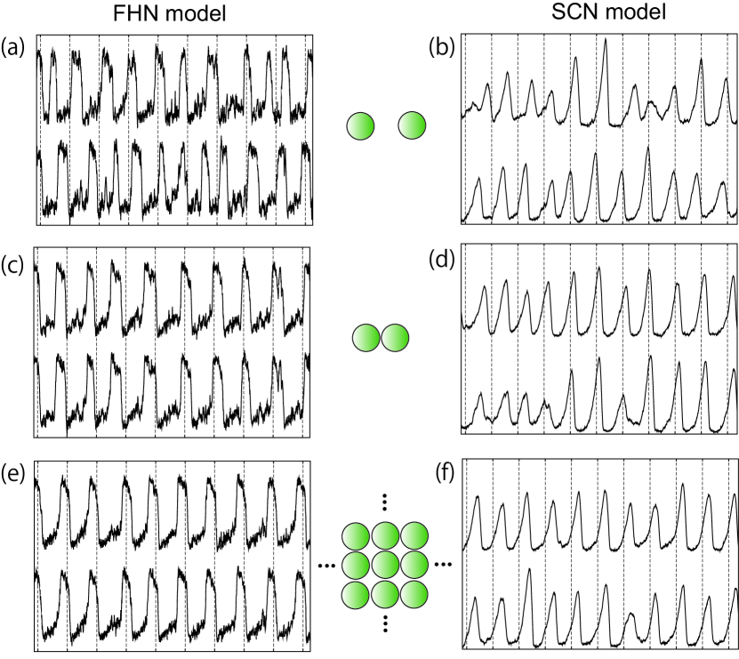
Figure 1: Waveforms obtained from biological oscillator models. We present the time series of $x_{i}(t)$ of (a,b) two isolated cells ($\kappa=0,N=2$), (c,d) two coupled cells ($\kappa>0,N=2$), and (e,f) two cells in 100 coupled cells ($\kappa>0,N=100$) in (a,c,e) the FHN model and (b,d,f) the SCN model. In (e), we employ the one-dimensional lattice with an open boundary condition and show the waveforms of two neighboring cells. In (f), we employ the all-to-all network ($A_{ij}=1/N$ for $1\leq i,j\leq N$). We set $\rho=0.1$ in all panels and (a,b) $\kappa=0$, (c,e) $\kappa=2$, and (d,f) $\kappa=1$.

Figures 1(a,c,e) and (b,d,f) present the waveforms obtained from the FHN and SCN models of different network sizes, respectively. The average cycle-to-cycle periods are depicted by dotted lines in each panel to illuminate the variations in cycle-to-cycle periods. The properties of each constituent cell were kept constant, while the connectivity between the cells is different. Typical waveforms of uncoupled cells ($N=2$) are shown in Figs. 1(a,b). When the cells are coupled sufficiently strongly, the system synchronizes stably (Figs. 1(c,d)). Figures 1(c,d) indicate that waveforms in the presence of coupling are regularized as compared to the waveforms of isolated cells [Figs. 1(a,b)]. In particular, the variation in the cycle-to-cycle period decreases. When 100 oscillators are coupled [Figs. 1(e,f)], the variation appears to be even smaller. When cells are coupled, individual cell oscillations are not only synchronized but also regularized, and the oscillation appears to be more regular for a larger system size.

There is a limit to the enhancement of temporal precision

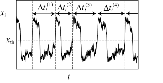
Figure 2: Schematic illustration of the concept of cycle-to-cycle period.

To quantify the dependence of temporal precision on network parameters, we measured the coefficient of variation (CV), which is the SD of the cycle-to-cycle period divided by the mean period. A cycle-to-cycle period is defined by an interval $\Delta t$ between two successive passages of an observed variable ($x_{i}$) across a specified threshold value $x_{\rm th}$ (Fig. 2). We set $x_{\rm th}=0.4$ and $2.0$ for the FHN and SCN models, respectively. We discard $\Delta t$ that is much smaller than a typical oscillation period to exclude noise-driven rapid threshold crossing. The CV is defined as

$${\rm CV}=\frac{\rm SD}{\rm\tau},$$ (1)

where $\tau$ and SD are the mean and the SD of a series of $\Delta t$, respectively.

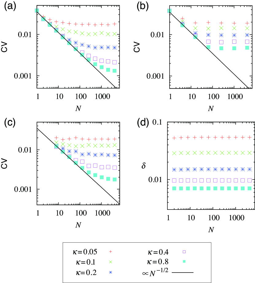
Figure 3: CV for single cell oscillations and synchronization distance $\delta$ in the FHN model. (a,b,c) CV values for single cell oscillations on (a) the all-to-all network, (b) the square lattice, and (c) the undirected random graph of size $N$. (d) Distance $\delta$ from in-phase synchrony in the all-to-all network. In (a) and (d), we set $A_{ij}=1/N$ for $1\leq i,j\leq N$. In (b), the CV of the oscillator at the center of the square lattice with an open boundary condition is presented. We set $A_{ij}=1/4$ with cell $j$ adjacent to cell $i$ and $A_{ij}=0$ otherwise. In (c), the CV value at given $\kappa$ and $N$ values is defined as $\langle{\rm CV}_{i}\rangle\equiv\sum_{i=1}^{N}{\rm CV}_{i}/N$ for a single realization of the network. We set $A_{ij}=A_{ji}=1/8$ with probability $p=8/N$ ($1\leq i<j\leq N$), and $A_{ij}=0$ otherwise. The lines are guides to the eyes. We considered identical cells and weak noise ($\rho=0.01$). The average period $\tau$ is almost constant $(\tau\approx 177)$ irrespective of $N$ and $\kappa$.

Here we investigate the FHN model on networks of different types and different sizes. We assume that the system is composed of identical cells subjected to weak noise. Figure 3(a) shows the CV of individual cell oscillations in the FHN model on the all-to-all network of size $N$. The results for different coupling strength values, $\kappa$, are plotted using different symbols. We find that

• CV is proportional to $1/\sqrt{N}$ for small $N$ values for each $\kappa$

• CV approaches a constant value for large $N$ values for each $\kappa$; i.e., there is a crossover

• the crossover point $N^{*}$ increases with $\kappa$.

We observe similar behavior for the square lattice and the random graph, as shown in Figs. 3(b) and (c), respectively.

Temporal precision increases with $N$, while the level of synchrony remains constant

A natural question is whether the enhanced synchronization induces the collective enhancement of temporal precision. To examine this possibility, we measured the distance $\delta$ between the actual state and the in-phase state (see Methods for the definition of $\delta$) for the all-to-all network. As shown in Fig. 3(d), the level of synchrony is independent of $N$ for each $\kappa$ value. We also confirmed that, in the FHN model on a square lattice, $\delta$ even increases with $N$ although the CV decreases (results not shown). Thus, the enhancement of temporal precision by an increase in $N$ is not attributed to the improvement in synchronization.

CV for ensemble activity has a larger crossover point

In nature, rhythmic output from a pacemaker organ is usually generated by an ensemble of multiple cells. For example, rhythmic electroactivity propagating within the heart is thought to originate from cells on the surface of the sinoatrial node. The SCN consists of various neural populations, and each population forms a particular pattern of efferent projections to other parts of the brain [19]. This anatomical fact suggests that the SCN’s output is generated by a combination of a subset of neurons rather than by the uniform average of the entire organ.

Therefore, we investigated the CV of the ensemble activity of a subset of cells on the all-to-all network. The ensemble activity is defined by the average waveform of $M$ ($1\leq M\leq N$) cells:

$$X(t)=\frac{1}{M}\sum_{i=1}^{M}x_{i}(t),$$ (2)

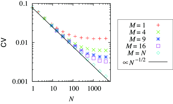
Figure 4: CV for ensemble activity of $M$ cells in the FHN model on the all-to-all network. Parameter values are the same as in Fig. 3, except $\rho=0.0256$ and $K=0.2$. The line is a guide to the eyes.

where the measured ensemble is assumed to consist of oscillators $x_{1}$, $\ldots$, $x_{M}$. The cycle-to-cycle period and the CV for the ensemble activity are defined similarly to the case of single cell activity (Fig. 2). In Fig. 4, we present the CV measured for the average waveform with different values of $M$ in the FHN model on the all-to-all network. For $M$ smaller than $N$, properties (i)–(iii) listed above are preserved. In addition, we find that

• the crossover point $N^{*}$ increases with ensemble size $M$

• for $M=N$, the CV is proportional to $1/\sqrt{N}$ for any $N$; i.e., there is no crossover.

We also confirmed that the same properties hold true for the FHN model on two–dimensional lattices and for the SCN model on the all-to-all network and the two–dimensional lattice.

Results are qualitatively the same under strong noise and heterogeneity

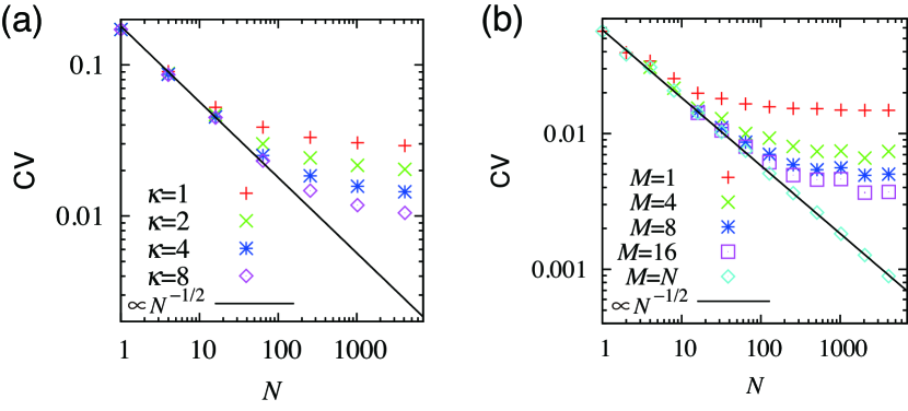
Figure 5: CV for biological models composed of heterogeneous cells subjected to relatively strong noise. (a) CV for single cell oscillations in the FHN model on the square lattice. We set $\rho=0.09$. (b) CV for the ensemble activity of $M$ cells in the SCN model on the all-to-all network. We set $\rho=0.04$ and $K=12$. The all-to-all network and the square lattice are the same as those in Figs. 3(a) and (b), respectively. The lines are guides to the eyes.

So far, we have assumed an ideal case: identical oscillators and weak noise. To simulate more realistic situations, we now consider networks composed of heterogeneous cells subjected to relatively strong noise. As examples, we measure the CV for the FHN model on the square lattice and for the SCN model on the all-to-all network (Fig. 5). In the FHN model, we made one of the parameter values heterogeneous in order to obtain the distribution of natural periods of cells as $\tau_{i}\approx 133\pm 3$ (mean $\pm$ SD). In the SCN model, the time scales of the cells were made heterogeneous such that $\tau_{i}\approx 23.4\pm 1.2$. The latter situation is consistent with the experimental observation by Honma et al. [20]. In all cases, we apply sufficiently strong coupling to ensure that the oscillators are well synchronized. Under this condition, as seen in Fig. 5, all properties (i)–(v) hold true.

Theory

We found, numerically, that properties (i)–(v) hold true in various situations. In the following, we develop a theory for relating temporal precision to network parameters by assuming weak coupling and weak noise. Under this assumption, a large class of oscillator systems including the models considered above are reduced to the phase model (see Methods and References [21, 22]) given by

$$\dot{\phi}_{i}(t)=\omega_{i}+\kappa\sum_{j=1}^{N}A_{ij}f(\phi_{j}-\phi_{i})+\sqrt{D}\xi_{i}(t),$$ (3)

where $\phi_{i}$ and $\omega_{i}$ $(1\leq i\leq N)$ are the phase and intrinsic frequency of the $i$th oscillator, respectively; $A=(A_{ij})$ is the weighted adjacency matrix with its element $A_{ij}$ equal to the intensity of the coupling from the $j$th to $i$th oscillators; $\kappa$ is the overall coupling intensity; $f(\cdot)$ is a $2\pi$–periodic function; $\xi_{i}(t)$ is independent white Gaussian noise with ${\rm E}[\xi_{i}(t)]=0$ and ${\rm E}[\xi_{i}(t)\xi_{j}(t^{\prime})]=\delta_{ij}\delta(t-t^{\prime})$, where ${\rm E}$ represents the expectation; and $D$ is the strength of the noise. The adjacency matrix $A$ is allowed to be asymmetric, weighted, and to possess negative components. Extension of the following results in the case of $i,j$-dependent coupling function $f_{ij}(\cdot)$ and $i$-dependent noise strength $D_{i}$ is straightforward. For clarity of the presentation, we focus on Eq. (3). We assume that all the oscillators are synchronized in frequency; i.e., all the oscillators have the actual frequency $\Omega$ owing to the effect of coupling. Synchronization usually occurs when coupling is sufficiently strong compared to noise and heterogeneity in $\omega_{i}$.

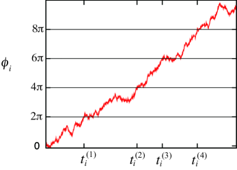
Figure 6: First passage time for a phase oscillator.

One oscillation cycle corresponds to an increase in the phase by $2\pi$. More precisely, the $k$th cycle-to-cycle period of the $i$th oscillator is defined by $\Delta t_{i}^{(k)}=t_{i}^{(k)}-t_{i}^{(k-1)}$, where $t_{i}^{(k)}$ is the first passage time for $\phi_{i}(t)$ to exceed $2k\pi$ (Fig. 6). Because we assumed that all the oscillators are synchronized to $\Omega$, the expected value of $\Delta t_{i}^{(k)}$ ($\tau$) is independent of $i$ and is given as

$$\tau\equiv{\rm E}[\Delta t_{i}^{(k)}]=\frac{2\pi}{\Omega},$$ (4)

where the statistical averages are taken over different $k$ values. The temporal precision of the $i$th oscillator is characterized by

$${\rm SD}_{i} \equiv{\rm std}[\Delta t_{i}]=\sqrt{{\rm var}[\Delta t_{i}]}=\sqrt{{\rm E}[(\Delta t_{i}^{(k)}-\tau)^{2}]}.$$ (5)

The CV for the $i$th oscillator is equal to

$${\rm CV}_{i}\equiv\frac{{\rm SD}_{i}}{\tau}.$$ (6)

To obtain the dependence of ${\rm SD}_{i}$ on network parameters, we employ an approximation given by

$$\frac{2\pi}{\tau}{\rm std}[\Delta t_{i}]\approx{\rm std}[\Delta\phi_{i}],$$ (7)

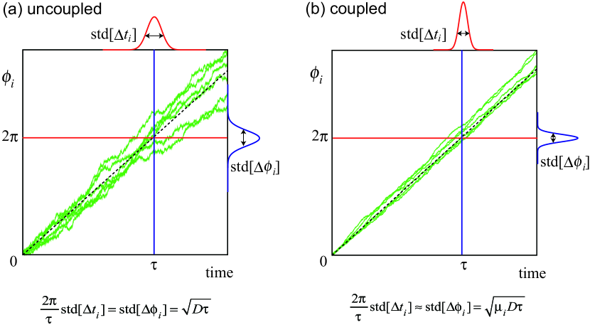
Figure 7: Schematic illustration of our approximation to the cycle-to-cycle variation. Green trajectories represent different realizations of the phase $\phi_{i}(t)$ of a single oscillator in (a) uncoupled and (b) coupled cases, where we set $\phi_{i}(0)=0$. The red curves on the top of each panel represent distribution function $P_{t}(t)$ obtained from the first passage time of $\phi_{i}(t)=2\pi$ in different realizations. Our concern is its standard deviation, ${\rm SD}_{i}={\rm std}[\Delta t_{i}]$. The blue curves on the right of each panel represent distribution function $P_{\phi}(\phi_{i})$ obtained from different realizations of $\phi_{i}(\tau)$, where $\tau$ is the mean period, and its standard deviation is denoted by ${\rm std}[\Delta\phi_{i}]$. We approximate ${\rm std}[\Delta t_{i}]$ using ${\rm std}[\Delta\phi_{i}]$. Suppose that $P_{t}(t)dt=P_{\phi}(\phi_{i})d\phi_{i}$. On average, the phase crosses $2\pi$ with slope $2\pi/\tau$, i.e., $d\phi_{i}/dt=2\pi/\tau$. We thus obtain Eq. (7). For uncoupled oscillators ($\kappa=0$), our model corresponds to the Wiener process with a constant drift. In this case, Eq. (7) is exact, and we obtain $(2\pi/\tau){\rm std}[\Delta t_{i}]={\rm std}[\Delta\phi]=\sqrt{D\tau}$ [37]. We also know that Eq. (7) is asymptotically exact in the one-dimensional Ornstein-Uhlenbeck process for weak noise [37]. For coupled oscillators $(\kappa>0)$, however, our model (3) is a multivariate Ornstein-Uhlenbeck process when linearized. Even in this case, as is numerically confirmed in the examples shown in Figs. 8–11, Eq. (7) provides a suitable approximation.

where $\Delta\phi_{i}\equiv\phi_{i}(t+\tau)-\phi_{i}(t)-2\pi$ (Fig. 7). For an isolated oscillator obeying $\dot{\phi}_{i}=\omega_{i}+\sqrt{D}\xi_{i}(t)$, one immediately finds that ${\rm var}[\Delta\phi_{i}]=D\tau_{i}$, where $\tau_{i}=2\pi/\omega_{i}$. When oscillators are coupled and synchronized with frequency $\Omega$, we write

$${\rm var}[\Delta\phi_{i}]=\mu_{i}D\tau.$$ (8)

We refer to $\mu_{i}$ as the scaling factor of the $i$th oscillator (Fig. 7).

To obtain an expression for $\mu_{i}$, we assume that noise is sufficiently weak and linearize Eq. (3) around the synchronized state. The synchronized solution $\phi_{i}^{\rm s}(t)$ $(1\leq i\leq N)$ is represented as

$$\phi_{i}^{\rm s}(t)=\Omega t+\psi_{i},$$ (9)

where $\Omega$ and $\psi_{i}$ are the constants derived by setting $\dot{\phi}_{i}=\Omega$ and $D=0$ in Eq. (3); i.e.,

$$\Omega=\omega_{i}+\kappa\sum_{j=1}^{N}A_{ij}f(\psi_{j}-\psi_{i}).$$ (10)

By introducing a small deviation

$$\theta_{i}(t)=\phi_{i}(t)-\phi_{i}^{\rm s}(t),$$ (11)

we obtain

$$\dot{\theta}_{i}(t)=\kappa\sum_{j=1}^{N}w_{ij}(\theta_{j}-\theta_{i})+\sqrt{D}\xi_{i}(t),$$ (12)

where $w_{ij}=A_{ij}f^{\prime}(\psi_{j}-\psi_{i})$ is the effective coupling weight. For convenience, we rewrite Eq. (12) as

$$\dot{\theta}_{i}(t)=-\kappa\sum_{j=1}^{N}L_{ij}\theta_{j}+\sqrt{D}\xi_{i}(t),$$ (13)

where $L=(L_{ij})$ is the Jacobian matrix with its element $L_{ij}$ given by

$$L_{ij}=\left\{\begin{array}[]{cl}-w_{ij}&\mbox{for $i\neq j$},\\ \sum_{i^{\prime}\neq i}w_{ii^{\prime}}&\mbox{for $i=j$}.\\ \end{array}\right.$$ (14)

Note that $L$ has a zero eigenvalue with the corresponding right eigenvector $\bm{u}^{(1)}=(1,\ldots,1)^{\top}/\sqrt{N}$. Furthermore, because of the assumption of the stability of the synchronized state, the real parts of the other $N-1$ eigenvalues of $L$ are positive, i.e., $0\equiv\lambda_{1}<{\rm Re}\lambda_{2}\leq\ldots\leq{\rm Re}\lambda_{N}$. The assumption of the stability holds true when $w_{ij}\geq 0$ ($1\leq i,j\leq N$) and the network described by the adjacency matrix $(w_{ij})$ is strongly connected [23, 24, 25]. For more general cases, the stability condition is nontrivial.

For in-phase synchrony (i.e., $\psi_{i}=0$ for $1\leq i\leq N$ in Eq. (9)), which occurs when the heterogeneity in the network and in individual oscillators is sufficiently small and/or the coupling is sufficiently strong, we obtain $w_{ij}\propto A_{ij}$ for $1\leq i,j\leq N$. In this case, $L$ is the network Laplacian generalized for a directed and weighted network [26], given by

$$L_{ij}\propto\left\{\begin{array}[]{cl}-A_{ij}&\mbox{for $i\neq j$},\\ \sum_{i^{\prime}\neq i}A_{ii^{\prime}}&\mbox{for $i=j$}.\\ \end{array}\right.$$ (15)

Note that $L$ is symmetric when the adjacency matrix $A$ is symmetric.

As shown in Methods, for any diagonalizable matrix $L$, we obtain $\mu_{i}=C_{ii}$, where

$$C_{ij} \equiv\frac{{\rm E}[(\theta_{i}(t+\tau)-\theta_{i}(t))(\theta_{j}(t+\tau)-\theta_{j}(t))]}{D\tau}$$

$$=\frac{V_{11}}{N}+\sum_{m,n\;(m+n>2)}^{N}\frac{2-e^{-\kappa\lambda_{m}\tau}-e^{-\kappa\lambda_{n}\tau}}{\kappa(\lambda_{m}+\lambda_{n})\tau}V_{mn}u^{(m)}_{i}u^{(n)}_{j}.$$ (16)

Here $\bm{u}^{(n)}=(u^{(n)}_{i})$ and $\bm{v}^{(n)}$ are, respectively, the right and left eigenvectors of $L$ that satisfy the orthogonality and normalization conditions; i.e., $L\bm{u}^{(n)}=\lambda_{n}\bm{u}^{(n)}$, $\bm{v}^{(n)}L=\lambda_{n}\bm{v}^{(n)}$, and $\bm{v}^{(m)}\bm{u}^{(n)}=\delta_{mn}$; and $V_{mn}=\bm{v}^{(m)}\cdot\bm{v}^{(n)}$.

For symmetric $L$, which is the case for in-phase synchrony on undirected networks, Eq. (16) becomes much simpler. Because all the eigenvalues are real, $\bm{u}^{(n)}=\bm{v}^{(n)\top}$, $V_{mn}=\bm{u}^{(m)}\cdot\bm{u}^{(n)}=\delta_{mn}$ for $1\leq m,n\leq N$, and $\sum_{i=1}^{N}u^{(n)}_{i}\propto\bm{u}^{(1)}\cdot\bm{u}^{(n)}=0$ for $n\geq 2$, we obtain

$$\mu_{i}=\frac{1}{N}+\sum_{n=2}^{N}\frac{1-e^{-\kappa\lambda_{n}\tau}}{\kappa\lambda_{n}\tau}u_{i}^{(n)}u_{i}^{(n)}.$$ (17)

Moreover, because of the normalization condition, $\sum_{i=1}^{N}u_{i}^{(n)}u_{i}^{(n)}=1$, the mean of $\mu_{i}$ over the entire network, $\langle\mu\rangle=\sum_{i=1}^{N}\mu_{i}/N$, is independent of the eigenvectors and is given by

$$\langle\mu\rangle=\frac{1}{N}+\frac{1}{N}\sum_{n=2}^{N}\frac{1-e^{-\kappa\lambda_{n}\tau}}{\kappa\lambda_{n}\tau}.$$ (18)

Crossover point $N^{*}$ increases with coupling strength $\kappa$

If the second term of Eq. (18) is negligible compared to the first term, we obtain $\langle\mu\rangle\approx 1/N$; i.e., the SD decreases proportionally to $1/\sqrt{N}$. However, as $N$ increases, the second term becomes comparable at certain $N^{*}$ and even dominant for $N\gg N^{*}$. If the eigenvalue spectrum converges to a certain density function $q(\lambda)$ as $N\to\infty$, we obtain

$$\langle\mu\rangle\to\mu_{\infty}\equiv\int_{0}^{\infty}q(\lambda)\frac{1-e^{-\kappa\lambda\tau}}{\kappa\lambda\tau}d\lambda\quad(N\to\infty).$$ (19)

We later demonstrate the convergence for the all-to-all and ring networks. Spectra of finite dimensional lattices [27], uncorrelated random graphs with arbitrary degree distributions [28], and the small-world network with a fixed expected degree [29] also converge. By equating the first and second terms in Eq. (18), we estimate the crossover point as $N^{*}\sim 1/\mu_{\infty}$. Since $\mu_{\infty}$ monotonically decreases with increasing $\kappa$, $N^{*}$ increases with $\kappa$.

Furthermore, if the second smallest eigenvalue $\lambda_{2}$ is nonvanishing in the limit $N\to\infty$ (which is the case, for example, in the all-to-all network and various random networks including small-world networks [29, 28]) and $\kappa$ is so large that $e^{-\kappa\lambda_{2}\tau}\ll 1$, we obtain $\mu_{\infty}\propto 1/\kappa$. Then, the crossover point scales as

$$N^{*}\propto\kappa.$$ (20)

Crossover point $N^{*}$ is proportional to the size of a measured ensemble

By assuming in-phase synchrony, we calculate the scaling factor of the noise reduction for the ensemble activity of an arbitrary set of oscillators. We rearrange the oscillator indices and write the ensemble activity as

$$X(t)=\sum_{i=1}^{M}\zeta_{i}x_{i}(t),$$ (21)

where $\zeta_{i}\geq 0$ is an arbitrary constant with the normalization condition $\sum_{i=1}^{M}\zeta_{i}=1$. When the deviation $\theta_{i}$ from in-phase synchrony (i.e., $\psi_{i}=0$ for $1\leq i\leq N$ in Eq. (9)) is small for each oscillator, the phase of $X(t)$ is approximated by

$$\Phi(t)=\sum_{i=1}^{M}\zeta_{i}\phi_{i}(t)=\Omega t+\sum_{i=1}^{M}\zeta_{i}\theta_{i}(t).$$ (22)

Then, similar to the case of individual cell oscillations, we define the scaling factor $\mu_{\Phi}$ for the ensemble activity as

$${\rm var}[\Delta\Phi]=\mu_{\Phi}D\tau,$$ (23)

where $\Delta\Phi=\Phi(t+\tau)-\Phi(t)-2\pi$. We then obtain

$$\mu_{\Phi}=\frac{{\rm var}[\Delta\Phi]}{D\tau}=\sum_{i,j=1}^{M}\zeta_{i}\zeta_{j}\frac{{\rm E}[(\theta_{i}(t+\tau)-\theta_{i}(t))(\theta_{j}(t+\tau)-\theta_{j}(t))]}{D\tau}=\sum_{i,j=1}^{M}\zeta_{i}\zeta_{j}C_{ij}.$$ (24)

Henceforth, we assume $\zeta_{i}=1/M$ for $1\leq i\leq M$, as is the case in Figs. 4 and 5(b).

There are notable properties for symmetric $L$ (see Methods). When $M=N$ (i.e., $X(t)$ is the mean activity of the entire network), we obtain

$$\mu_{\Phi}=\frac{1}{N},$$ (25)

that is, there is no crossover. For $M<N$, $\mu_{\Phi}$ generally depends on the choice of $M$ oscillators. However, if we randomly choose $M$ oscillators out of $N$ oscillators, where $1\ll M\ll N$, we estimate

$$\mu_{\Phi}\approx\frac{1}{N}+\frac{1}{MN}\sum_{n=2}^{N}\frac{1-e^{-\kappa\lambda_{n}\tau}}{\kappa\lambda_{n}\tau}\approx\frac{1}{N}+\frac{\mu_{\infty}}{M}.$$ (26)

In this case, the lower bound of the SD is inversely proportional to $\sqrt{M}$ and the crossover point increases as

$$N^{*}\propto M.$$ (27)

As shown later, this estimation is asymptotically exact for the all-to-all network.

Behavior $1/\sqrt{N}$ can be violated even for small $N$ values when $L$ is asymmetric

The behavior ${\rm CV}\propto 1/\sqrt{N}$ is obtained for $N<N^{*}$ when the Jacobian $L$ is symmetric, which is the case when a network is undirected and the oscillators are synchronized in phase. We refer to this situation as “democratic” because symmetric $L$ implies that the action and reaction between any two nodes are balanced.

For asymmetric $L$, Eq. (16) implies that the SD at small $N$ values decreases as $\sqrt{V_{11}/N}$ instead of $1/\sqrt{N}$. In [30], we analyzed the long-time diffusion property of Eq. (3) to obtain $\sigma^{2}\equiv\lim_{\Delta t\to\infty}{\rm var}[\theta_{i}(t+\Delta t)-\theta_{i}(t)]/(D\Delta t)=V_{11}/N$ through a different technique. This previous result is consistent with that obtained in the present paper because $\sigma^{2}$ corresponds to phase diffusion after infinitely many cycles, and the second term on the right-hand side of Eq. (16) vanishes with this limit. Furthermore, we showed in [30] that $\sqrt{V_{11}/N}$ is larger than or equal to $1/\sqrt{N}$ for asymmetric $L$. For example, in directed scale-free networks, which is a strongly heterogeneous network, we obtained $\sqrt{V_{11}/N}\propto N^{-\beta}$ with $0\leq\beta\leq 1/2$; the effect of collective enhancement is significantly weaker. Moreover, the scaling $\sqrt{V_{11}/N}=N^{-1/2}$ can be violated even when a network is undirected. This is the case when the synchronized state is not in-phase but accompanies a wave pattern. Wave patterns arise when the network is spatially extended (such as Euclidian lattices) and the natural frequency is sufficiently heterogeneous [22, 31]. In this case, $V_{11}/N$ decreases with $N$ for small $N$ values but approaches a constant value for large $N$ values. Thus, strongly asymmetric connectivity and/or strong heterogeneity in the oscillator’s properties can hamper the collective enhancement of temporal precision.

Examples and numerical verification

To demonstrate and numerically confirm our analytical results, we investigate the phase model (Eq. (3)) on several networks. In numerical simulations, we set $\omega_{i}=1$, $f(\phi)=\sin\phi$, and $\sqrt{D}=0.01$ in Eq. (3). In the example networks, all the oscillators synchronize in phase in the absence of noise. Thus, $w_{ij}=A_{ij}$ and $\Omega=\omega$ for any coupling strength $\kappa$ and any $N$. Note that the dependence of the CV on $\kappa$ and $N$ is only through the SD because $\tau=2\pi/\omega$ is constant. In the following, we show the values of the normalized CV, that is actual CV values divided by the CV of isolated oscillators, shown as $\sqrt{D\tau}/2\pi$. Our theory predicts that ${\rm CV}_{i}\approx\sqrt{\mu_{i}}$ and ${\rm CV}_{\Phi}\approx\sqrt{\mu_{\Phi}}$.

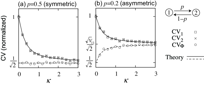
Figure 8: Normalized CV versus coupling strength in asymmetrically coupled phase oscillators ($N=2$). Presented is the normalized CV, i.e., ${\rm CV}_{i}/(\sqrt{D\tau}/2\pi)$ $(i=1,2)$ and ${\rm CV}_{\Phi}/(\sqrt{D\tau}/2\pi)$ for two coupled phase oscillators with (a) $p=0.5$ and (b) $p=0.2$. Numerical results are shown by symbols. The solid and dotted lines represent the analytical results given by Eqs. (28) and (29), respectively. Note that $V_{11}=2p^{2}+2(1-p)^{2}=1$ for $p=0.5$ and $V_{11}=1.36$ for $p=0.2$.

Two asymmetrically coupled elements. The first example is two asymmetrically coupled elements ($N=2$): $w_{12}=p$ and $w_{21}=1-p$ (Fig. 8). In this case, we have $\lambda_{1}=0,\lambda_{2}=-1,\bm{u}^{(1)}=\frac{1}{\sqrt{2}}(1\;1)^{\top},\bm{v}^{(1)}=\sqrt{2}(p\;1-p),\bm{u}^{(2)}=\sqrt{2}(1-p\;-p)^{\top}$, and $\bm{v}^{(2)}=\frac{1}{\sqrt{2}}(1\;-1)$. By substituting them in Eqs. (16) and (24) for $M=2$ and setting $\zeta_{1}=\zeta_{2}=1/2$, we obtain

$$\mu_{1} =\mu_{2}=\frac{V_{11}}{2}+\left(1-\frac{V_{11}}{2}\right)\frac{1-e^{-\kappa\tau}}{\kappa\tau},$$ (28)

$$\mu_{\Phi} =\frac{V_{11}}{2}+\left(\frac{1}{2}-\frac{V_{11}}{2}\right)\frac{1-e^{-\kappa\tau}}{\kappa\tau},$$ (29)

where $V_{11}=2p^{2}+2(1-p)^{2}$. For any $\kappa$ and $\tau$ values, the best precision is obtained in the symmetric case ($p=0.5$). Figure 8 suggests that the analytical and numerical results are in strong agreement.

All-to-all coupling. The second example is all-to-all coupling; i.e., $w_{ij}=1/N$ for $1\leq i,j\leq N$. The eigenvalues are given by $\lambda_{n}=1$ ($2\leq n\leq N$). Because all the nodes are equivalent (i.e., permutation symmetry), we obtain $\mu_{i}=\langle\mu\rangle$. Then, from Eq. (18), it follows that

$$\mu_{i}=\frac{1}{N}+\left(1-\frac{1}{N}\right)\frac{1-e^{-\kappa\tau}}{\kappa\tau}.$$ (30)

We also obtain a concise form for $\mu_{\Phi}$ (see Methods), given by

$$\mu_{\Phi}=\frac{1}{N}+\left(\frac{1}{M}-\frac{1}{N}\right)\frac{1-e^{-\kappa\tau}}{\kappa\tau}.$$ (31)

We denote the CV value at $N=N^{*}$ by ${\rm CV}^{*}$. By equating the first and second terms on the right-hand side in Eq. (31) and assuming $M\ll N$ and $e^{-\kappa\tau}\ll 1$, we obtain

$$N^{*}\approx\kappa\tau M,\quad{\rm CV}^{*}\propto\frac{1}{\sqrt{\kappa\tau M}}.$$ (32)

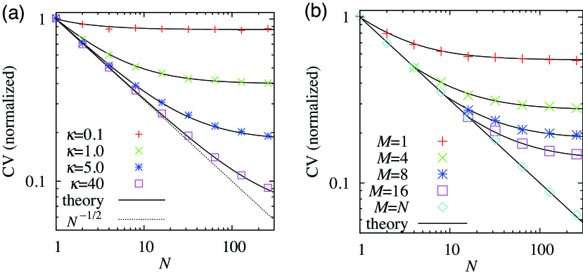
Figure 9: Normalized CV in phase oscillators on the all-to-all network. (a) CV for individual cells ($M=1$) for various $\kappa$ and $N$ values. (b) CV for ensemble activity for various $M$ values with $\kappa=0.5$. Symbols represent numerical data. Solid lines represent (a) $\sqrt{\mu_{i}}$ given by Eq. (30) and (b) $\sqrt{\mu_{\Phi}}$ given by Eq. (31).

Figure 9 shows the analytical and numerical results. Note that in Figs. 4 and 5(b), the lower bounds are roughly proportional to $1/\sqrt{M}$, as our theory predicts.

Ring. The third example is the ring of size $N$, i.e., $w_{i,i+1}=w_{i,i-1}=1/2$ for $1\leq i\leq N$ and $w_{i,j}=0$ for $j\neq i-1,i+1$, as an example of spatially extended systems. For this network, we obtain

$$\lambda_{n}=1-\cos\left(\frac{2(n-1)\pi}{N}\right)$$ (33)

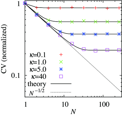
Figure 10: Normalized CV for single cells in phase oscillators on the ring. Symbols represent numerical results. Solid lines represent $\sqrt{\mu_{i}}$ given by Eq. (18) with Eq. (33).

for $1\leq n\leq N$. Because $L$ is symmetric and the network has permutation symmetry, we obtain $\mu_{i}=\langle\mu\rangle$ where $\langle\mu\rangle$ is given by Eqs. (18) and (33). Figure 10 shows the analytical and numerical results. Although each cell is adjacent to just two cells for any $N\geq 3$, there is a clear $N$-dependence of the CV for individual cells. Temporal precision is not simply determined by local connectivity.

The lower bound of the CV for the ring is considerably larger than that for the all-to-all network (Figs. 9(a) and 10). The reason for this is as follows. The Laplacian of the ring for a large $N$ value has negligible eigenvalues (i.e., $\lambda_{n}$ for $n\approx 0$ and $n\approx N$ in Eq. (33)), and these eigenvalues significantly enlarge the second term of Eq. (18). In contrast, there is a nonvanishing spectrum gap (i.e., the second smallest eigenvalue $\lambda_{2}$) in the all-to-all and various random networks [29, 28]. In the FHN model, we observed a similar difference between the cases of the square lattice (Fig. 3(b)) and the all-to-all and random networks (Figs. 3(a) and (c), respectively). This is also because the square lattice has negligible eigenvalues [27]. Such small eigenvalues are associated with slow synchronization of remote oscillators owing to a time lag in communication, and this property is shared by any spatially extended networks with local interaction. Therefore, spatial networks with only local interaction are disadvantageous to temporal precision.

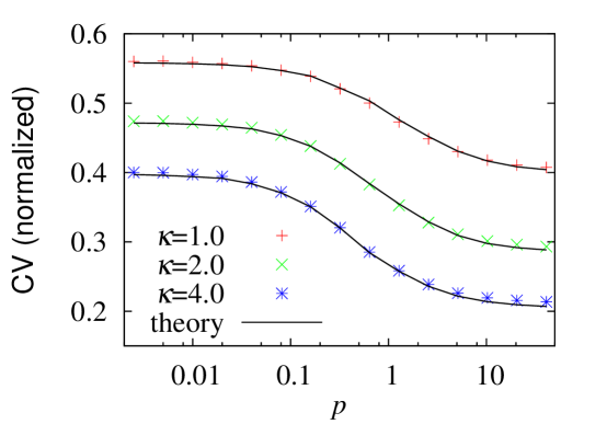
Figure 11: Normalized CV for individual cells in phase oscillators on the variant of the Watts-Strogatz model. We present $\langle{\rm CV}_{i}\rangle/(\sqrt{\tau D}/2\pi)$, where $\langle{\rm CV}_{i}\rangle\equiv\sum_{i=1}^{N}{\rm CV}_{i}/N$. Lines represent $\sqrt{\mu_{i}}$ given by Eq. (17). We set $N=400$.

Small-world networks. By using a type of the Watts-Strogatz model [32, 33] of fixed size $N$, we demonstrate that a small fraction of long-range interactions added to the ring drastically improves temporal precision. We generate a network by adding $pN$ bidirectional shortcuts sequentially to the ring, where $p$ is the shortcut density. Under the condition that multiple links are avoided, the two endpoints of each shortcut are chosen from the $N$ nodes with equal probability. The generated network is undirected. To maintain the total coupling strength independent of $p$, we set $w_{ij}=w_{ji}=1/(2+2p)$ for all links. The ring and all-to-all networks are obtained at $p=0$ and $p=N/2-1$, respectively. Figure 11 shows the numerically obtained $\langle{\rm CV}\rangle$ for each $p$, where $\langle{\rm CV}\rangle\equiv\sum_{i=1}^{N}{\rm CV}_{i}/N$ for a single realization of the network. The lines represent $\sqrt{\langle\mu\rangle}$ obtained from Eq. (18), where we numerically computed the eigenvalues $\lambda_{n}$ for the generated network We set the coupling strength such that $\langle\mu\rangle\gg 1/N$ (i.e., $N\gg N^{*}$) for the initial ring ($p=0$).

Figure 11 indicates that temporal precision is considerably improved at $p\approx 1$, i.e., when $O(N)$ shortcuts are added (the small-world regime). Moreover, the corresponding CV value is close to that of the all-to-all network, in which $O(N^{2})$ “shortcuts” exist. As discussed above, there are small eigenvalues that hamper temporal precision in spatially extended networks. Such small eigenvalues do not exist in networks with a sufficient number of shortcuts because of rapid communication between any pair of oscillators.

Mechanism of the crossover

We demonstrated using various models that the crossover generally occurs in the collective enhancement. On the basis of our theory, the crossover can be interpreted as follows. When Jacobian $L$ is symmetric, the SD for the mean phase decreases as $1/\sqrt{N}$ for any $N$ (Eq. (25)). When coupling strength $\kappa$ is infinite, the oscillators are completely synchronized in phase. Then, the phase of each oscillator is identical with the mean phase, and so is the SD, i.e., ${\rm SD}_{i}\propto 1/\sqrt{N}$ for any $N$. This behavior is expressed in the first term on the right-hand side of Eq. (17). However, for finite $\kappa$, individual oscillators’ phases fluctuate around the mean phase because of the independent noise applied to the oscillators. Owing to this additional fluctuation, the SD for individual oscillators is larger than that for the mean phase, as expressed in the second term on the right-hand side of Eq. (17). Although the fluctuation in the mean phase vanishes with the limit $N\to\infty$, it remains finite in individual oscillators. This is the origin of the lower bound.

Discussion

We found that the collective enhancement is ineffective for system size $N$ above the crossover point $N^{*}$. We further showed that $N^{*}$ increases with coupling strength (Eq. (20)). Therefore, as oscillators are more strongly coupled, the behavior ${\rm CV}\propto 1/\sqrt{N}$ persists up to a larger $N$ value. This is the case for different oscillation and coupling mechanisms, as demonstrated in the two biological models (the FHN and SCN models) and the phase oscillator model. Moreover, this behavior also holds true for different network connectivities, as demonstrated using the ring, the square lattice, the all-to-all network, and the random graph.

Our theory is useful for inferring the magnitude of fluctuations in individual cells and the coupling strength between cells. Suppose that temporal precision in a pacemaker tissue that is genetically modified or subjected to a treatment (e.g., drug) is lower than that in an intact tissue. If the cells in the tissue are well synchronized in both cases, one may consider that the treatment affects the oscillation mechanism of individual cells. Our theory suggests another possibility: a decrease in the coupling strength, not the alteration in the oscillation property of individual cells, may be the reason for the reduced temporal precision (Figs. 3(a,b,c)). By observing reduced temporal precision only, we cannot distinguish these two possibilities. However, our theory makes it possible to individually quantify the effects of the treatment on the two properties if we can observe cell networks of different sizes. By observing temporal precision in small (i.e., $N<N^{*}$) tissues of different sizes, we can infer the magnitude of fluctuations in individual cells by fitting the law ${\rm CV}\propto 1/\sqrt{N}$. Furthermore, by observing relatively large tissues and determining $N^{*}$ values for different treatments (e.g., different days of cultivation, different concentrations of a drug, treated versus untreated), we can infer changes in the coupling strength induced by the treatment because $N^{*}$ increases with the coupling strength (Eq. (20)).

Our study also indicates that long-range interactions among cells are advantageous to temporal precision. As demonstrated in Fig. 11, the addition of shortcut links considerably decreases the CV. A similar result was reported in a previous numerical study using a more realistic model for the SCN [13]. This result might underlie an evolutionary origin of dense fibers across the SCN [19].

Our theoretical results provide an interpretation of previous experiments on cardiac and circadian oscillations. Kojima et al observed a decrease in the CV with increasing cell number in cultivated cardiac cells coupled via micro channels [9]. They showed that the CV decreases considerably with $N$ for small $N$ values ($N=1,2,3$), while it is almost constant for $N\geq 4$. In contrast, in cultivated cardiac cells that are directly and tightly coupled to each other, Clay and DeHaan found that the reduction in the CV roughly obeys ${\rm CV}\propto 1/\sqrt{N}$ up to $N\approx 100$ [6]. Although the cells are kept synchronized in both cases, the behavior of temporal precision is different. This discrepancy may be due to a difference in coupling strength. While the coupling was strong enough to guarantee synchrony in both cases, coupling in the latter experiments may be stronger than that in the former experiments, resulting in $N^{*}\approx 4$ and $N^{*}>100$, respectively. It would be of great interest to investigate systematically how the crossover point increases with coupling strength, possibly controlled by the width of the micro channel implemented in the former experiments [9].

Collective enhancement has been examined experimentally in circadian oscillation as well. Herzog et al measured temporal precision in SCN cells [8]. There, individual cell oscillations in both synchronized and unsynchronized cases were observed in slice cultures of SCN and dispersed SCN cells, respectively. They found that the SD in the former (0.42 h) was approximately five times smaller than that in the latter (2.1 h), and argued that the collective enhancement of temporal precision occurs in synchronized cells. They further speculated that, under the assumption ${\rm SD}\approx 1/\sqrt{N}$, only 25 cells out of the order of $10^{5}$ cells composing the SCN are involved in the collective enhancement of temporal precision in the explant SCN.

We interpret this experimental result as follows. In the SCN, a wave pattern is observed [34, 35]. As indicated above as well as in our previous paper [30], the law ${\rm SD}\propto 1/\sqrt{N}$ is violated in the presence of a wave pattern even if the coupling is sufficiently strong. Roughly speaking, the reason for this is that only the cells forming the source of the wave pattern can contribute to the collective enhancement of temporal precision, and other cells simply obey those cells [30]. The number of cells forming the source might be of the order of 25. Cells located downstream of the wave may contribute to functions other than temporal precision.

Our theory is widely applicable to frequency-synchronized oscillators with weak noise and weak coupling. Our theory can also apply to the case of the coexistence of multiple coupling mechanisms, only by replacing coupling function $f$ by $f_{ij}$ in the phase model (Eq. (3)). Although the phase model is not justified when the assumption of weak noise and weak coupling is violated, we have numerically confirmed that our main finding, i.e., the properties (i)–(v), are preserved in the case of strong coupling and strong noise (Fig. 5). We thus expect that our theory, based on the phase model, captures the essence of the collective enhancement of temporal precision.

Methods

Model equations for biological pacemaker systems

We consider two systems—the FHN model and the SCN model representing the cardiac pacemaker organ and the circadian master clock, respectively.

The FHN model has been extensively used as a model of neurons and cardiac cells [36]. Our FHN model is given by

$$\frac{dx_{i}}{dt} =x_{i}(a-x_{i})(x_{i}-1)-y_{i}+\rho\xi_{i}(t)+\kappa\sum_{j=1}^{N}A_{ij}(x_{j}-x_{i}),$$ (34a)

$$\frac{dy_{i}}{dt} =\epsilon(x_{i}-by_{i}+c),$$ (34b)

where $a,b,c,\epsilon$ are the model parameters, $\rho$ is the noise strength, $\xi_{i}(t)$ is white Gaussian noise with ${\rm E}[\xi_{i}(t)]=0$ and ${\rm E}[\xi_{i}(t)\xi_{j}(t^{\prime})]=\delta_{ij}\delta(t-t^{\prime})$. We chose parameter values such that each unit is autonomous oscillator. In Figs. 1, 3 and 4, we set $a=0.1,\epsilon=0.01,b=0.5$, and $c=0.05$. In Fig. 5(a), we replace $c$ with $c_{i}=0.1+0.02\nu_{i}$ ($1\leq i\leq N$), where $\nu_{i}$ is a random variable independently taken from the Gaussian distribution with zero mean and unit variance. We varied the noise strength and coupling strength, as specified in the figures and their captions. The distance $\delta$ from the in-phase state is defined as

$$\delta=\sqrt{\frac{1}{N-1}\sum_{i=1}^{N}(x_{i}-\overline{x})^{2}},$$ (35)

where $\overline{x}=\sum_{i=1}^{N}x_{i}/N$.

As the SCN model, we employed a previously proposed model [18], given by

$$\frac{dx_{i}}{dt} =T_{i}\left(V_{1}\frac{K_{1}^{n}}{K_{1}^{n}+z_{i}^{n}}-V_{2}\frac{x_{i}}{K_{2}+x_{i}}+V_{c}\frac{\kappa F_{i}}{K_{c}+\kappa F_{i}}\right)+\rho\xi_{i}^{(x)},$$ (36a)

$$\frac{dy_{i}}{dt} =T_{i}\left(k_{3}x_{i}-V_{4}\frac{y_{i}}{K_{4}+y_{i}}\right)+\rho\xi_{i}^{(y)},$$ (36b)

$$\frac{dz_{i}}{dt} =T_{i}\left(k_{5}y_{i}-V_{6}\frac{z_{i}}{K_{6}+z_{i}}\right)+\rho\xi_{i}^{(z)},$$ (36c)

$$\frac{dr_{i}}{dt} =T_{i}\left(k_{7}x_{i}-V_{8}\frac{r_{i}}{K_{8}+r_{i}}\right)+\rho\xi_{i}^{(r)},$$ (36d)

$$F_{i} =\sum_{j=1}^{N}A_{ij}r_{j},$$ (36e)

where $V_{1}=6.8355,n=5.6645,K_{1}=2.7266,K_{2}=0.2910,k_{3}=0.1177,V_{4}=1.0841,K_{4}=8.1343,k_{5}=0.3352,V_{6}=4.6645,K_{6}=9.9849,k_{7}=0.2282,V_{8}=3.5216,K_{8}=7.4519,V_{c}=6.7924,K_{c}=4.8283,\kappa=12.0$, and $V_{2}=12.0$. All parameter values except for $\kappa$ and $V_{2}$ are taken from [18]. Time constant $T_{i}$ is introduced to express heterogeneity in the oscillation period. We set $T_{i}=1$ in Fig. 1. In Fig. 5(b), $T_{i}=1+0.05\nu_{i}$ with $\nu_{i}$ independently obeying the Gaussian distribution with zero mean and unit variance. The functions $\xi_{i}^{(\zeta)}(t)$ ($\zeta=x,y,z,r$) represent white Gaussian noise processes with ${\rm E}[\xi_{i}^{(\zeta)}(t)]=0$ and ${\rm E}[\xi_{i}^{(\zeta)}(t)\xi_{j}^{(\eta)}(t^{\prime})]=\delta_{ij}\delta_{\zeta\eta}\delta(t-t^{\prime})$. The noise strength $\rho$ and coupling strength $\kappa$ are specified in the figures and their captions.

In both models, we applied sufficiently strong coupling to ensure that the oscillators were synchronized nearly in phase. When we computed the CV, we assumed random initial conditions and measured a sufficiently large number of cycle-to-cycle periods after the transient.

Networks

The all-to-all network used in Figs. 1(b,d,f), 3(a,d), 4, 5(b), and 9 is defined by $A_{ij}=1/N$ for $1\leq i,j\leq N$. The one-dimensional lattice with an open boundary condition used in Fig. 1(e) is defined by $A_{ij}=1/2$ for $1\leq i\leq N$ and $1\leq j=i\pm 1\leq N$, and $A_{ij}=0$ otherwise. The ring used in Fig. 10 is the same as the one-dimensional lattice except that we impose a periodic boundary condition $A_{1,N}=A_{N,1}=1/2$. The square lattice with an open boundary condition used in Figs. 3(b) and 5(a) is defined by $A_{ij}=1/4$ with cell $j$ adjacent to $i$ for $1\leq i,j\leq\sqrt{N}$ and $A_{ij}=0$ otherwise. The undirected random graph used in Fig. 3(c) is the Erdős-Rényi random graph, where $A_{ij}=A_{ji}=1/8$ for $1\leq i<j\leq N$ with probability $p=8/N$ and $A_{ij}=A_{ji}=0$ otherwise. We set link weights such that the summed weight of the links per node is independent of $N$; i.e., for $1\leq i\leq N$, $\sum_{j=1}^{N}A_{ij}=1$ in the ring and all-to-all network and $\sum_{j=1}^{N}A_{ij}\approx 1$ in the other networks including the Watts-Strogataz model used in Fig. 11.

Phase description

A large class of oscillator systems including the FHN and SCN models (Eqs. (34) and (36)) are reduced to phase models if the coupling and noise are sufficiently weak [21, 22]. The concept behind the reduction is as follows. We denote an element of the state variable of the $i$th oscillator by $x_{i}(t)$. When unperturbed, the oscillator portrays a one-dimensional closed orbit after transient so that $x_{i}(t)=x_{i}(t+2\pi/\omega_{i})$, where $\omega_{i}$ is the intrinsic frequency. We define the phase $\phi_{i}$ by $x_{i}(t)=x_{i}(\phi_{i}/\omega_{i})$; that is, the phase increases linearly with time in the unperturbed oscillator. For convenience, we denote the unperturbed orbit by $\chi(\phi_{i})=x_{i}(\phi_{i}/\omega_{i})$. Although the trajectory deviates from the closed orbit when the oscillator is weakly perturbed, it is still possible to parameterize a trajectory of an oscillator by only the phase and describe the dynamics of coupled oscillators in terms of the phases only [21, 22]. The resulting equation is given by Eq. (3). Because of the assumption of weak perturbation, $x_{i}(t)$ is approximated by that of the unperturbed orbit, i.e.,

$$x_{i}(t)\approx\chi(\phi_{i}(t)).$$ (37)

Therefore, the first passage time problem for $x_{i}(t)$ is approximated by that for $\phi_{i}{\color[rgb]{0,0,1}(}t)$.

Calculation of Eq. (16)

Our linearized equation is given by Eq. (13), which is reproduced as

$$\dot{\theta}_{i}(t)=-\kappa\sum_{j=1}^{N}L_{ij}\theta_{j}+\sqrt{D}\xi_{i}(t),$$ (38)

where $\theta_{i}$ ($1\leq i\leq N$) is the deviation from the synchronized state, $\kappa>0$ is the coupling strength, $L=(L_{ij})$ is a diagonalizable matrix, and $\xi_{i}(t)$ is white Gaussian noise with

$${\rm E}\left[\xi_{i}(t)\right]=0,\quad{\rm E}\left[\xi_{i}(t)\xi_{j}(s)\right]=\delta_{ij}\delta(t-s).$$ (39)

From the assumption of the stability of frequency synchronization, we have

$$0=\lambda_{1}<{\rm Re\,}\lambda_{2}\leq{\rm Re\,}\lambda_{3}\leq\cdots\leq\lambda_{N}.$$ (40)

The right and left eigenvectors of $L$ corresponding to $\lambda_{n}$ are denoted by $\bm{u}^{(n)}=(u_{i}^{(n)})$ and $\bm{v}^{(n)}=(v_{i}^{(n)})$, respectively; i.e.,

$$L\bm{u}^{(n)} =\lambda_{n}\bm{u}^{(n)},$$ (41a)

$$\bm{v}^{(n)}L =\lambda_{n}\bm{v}^{(n)}$$ (41b)

with the normalization and orthogonality conditions

$$\bm{v}^{(m)}\bm{u}^{(n)}=\delta_{mn}.$$ (42)

Using these eigenvectors, we decompose $\theta_{i}(t)$ as

$$\theta_{i}(t)=\sum_{m=1}^{N}\varphi_{m}(t)u_{i}^{(m)},$$ (43)

where $\varphi_{m}(t)$ is given by

$$\varphi_{m}(t)=\sum_{i=1}^{N}\theta_{i}(t)v_{i}^{(m)}.$$ (44)

By taking the time derivative of Eq. (44) and using Eqs. (38), (42) and (43), we obtain

$$\dot{\varphi}_{m}(t)=-\kappa\lambda_{m}\varphi_{m}+\eta_{m}(t),$$ (45)

where

$$\eta_{m}(t)=\sqrt{D}\sum_{i=1}^{N}v_{i}^{(m)}\xi_{i}(t).$$ (46)

Equation (39) yields $\left\langle\eta_{m}(t)\right\rangle=0$. We also have

$${\rm E}\left[\eta_{m}(t)\eta_{n}(s)\right] ={\rm E}\left[D\sum_{i=1}^{N}v_{i}^{(m)}\xi_{i}(t)\sum_{j=1}^{N}v_{j}^{(n)}\xi_{j}(s)\right]$$

$$=D\sum_{i,j=1}^{N}v_{i}^{(m)}v_{j}^{(n)}{\rm E}\left[\xi_{i}(t)\xi_{j}(s)\right]$$

$$=D\sum_{i,j=1}^{N}v_{i}^{(m)}v_{j}^{(n)}\delta_{ij}\delta(t-s)$$

$$=D\left(\sum_{i=1}^{N}v_{i}^{(m)}v_{i}^{(n)}\right)\delta(t-s)$$

$$=DV_{mn}\delta(t-s),$$ (47)

where

$$V_{mn}\equiv\sum_{i=1}^{N}v_{i}^{(m)}v_{i}^{(n)}.$$ (48)

Now we derive $C_{ij}$ given in Eq. (16). The definition of $C_{ij}$ is

$$C_{ij}\equiv\frac{1}{D\tau}{\rm E}[(\theta_{i}(t+\tau)-\theta_{i}(t))(\theta_{j}(t+\tau)-\theta_{j}(t))].$$ (49)

By substituting Eq. (43) in Eq. (49), we obtain

$$C_{ij}=\frac{1}{D\tau}\sum_{m,n=1}^{N}u_{i}^{(m)}u_{j}^{(n)}{\rm E}\left[(\varphi_{m}(t+\tau)-\varphi_{m}(t))(\varphi_{n}(t+\tau)-\varphi_{n}(t))\right].$$ (50)

The solution to Eq. (45) is formally written as

$$\varphi_{m}(t)=e^{-\kappa\lambda_{m}t}\varphi_{m}(0)+\int_{0}^{t}ds\,e^{-\kappa\lambda_{m}(t-s)}\eta_{m}(s).$$ (51)

Using Eq. (51), we obtain

$$\varphi_{1}(t+\tau)-\varphi_{1}(t)=\int_{t}^{t+\tau}ds\,\eta_{1}(s),$$ (52)

$${\rm E}\left[(\varphi_{1}(t+\tau)-\varphi_{1}(t))(\varphi_{1}(t+\tau)-\varphi_{1}(t))\right] =\int_{t}^{t+\tau}ds_{1}\int_{t}^{t+\tau}ds_{2}\,{\rm E}\left[\eta_{1}(s_{1})\eta_{1}(s_{2})\right]$$

$$=DV_{11}\int_{t}^{t+\tau}ds_{1}\int_{t}^{t+\tau}ds_{2}\,\delta(s_{1}-s_{2})$$

$$=DV_{11}\tau.$$ (53)

To evaluate the terms on the right-hand side of Eq. (50) for $m+n>2$, we first calculate

$$B_{mn}(t_{1},t_{2}) \equiv\int_{0}^{t_{1}}ds_{1}\int_{0}^{t_{2}}ds_{2}\,e^{-\kappa\lambda_{m}(t_{1}-s_{1})-\kappa\lambda_{n}(t_{2}-s_{2})}{\rm E}\left[\eta_{m}(s_{1})\eta_{n}(s_{2})\right]$$

$$=\int_{0}^{t_{1}}ds_{1}\int_{0}^{t_{2}}ds_{2}\,e^{-\kappa\lambda_{m}(t_{1}-s_{1})-\kappa\lambda_{n}(t_{2}-s_{2})}DV_{mn}\delta(s_{1}-s_{2})$$

$$=DV_{mn}\int_{0}^{\min(t_{1},t_{2})}ds\,e^{-\kappa\lambda_{m}(t_{1}-s)-\kappa\lambda_{n}(t_{2}-s)}$$

$$\to DV_{mn}\left.\frac{e^{-\kappa\lambda_{m}(t_{1}-s)-\kappa\lambda_{n}(t_{2}-s)}}{\kappa(\lambda_{m}+\lambda_{n})}\right|_{s=\min(t_{1},t_{2})}.$$ (54)

We consider the limit $t\to\infty$ in Eq. (54) because we are concerned with a stationary process. Using Eq. (54), we obtain

$${\rm E}\left[(\varphi_{m}(t+\tau)-\varphi_{m}(t))(\varphi_{n}(t+\tau)-\varphi_{n}(t))\right]$$

$$=B_{mn}(t+\tau,t+\tau)-B_{mn}(t+\tau,t)-B_{mn}(t,t+\tau)+B_{mn}(t,t)$$

$$\to DV_{mn}\frac{2-e^{-\kappa\lambda_{m}\tau}-e^{-\kappa\lambda_{n}\tau}}{\kappa(\lambda_{m}+\lambda_{n})}\quad(t\to\infty).$$ (55)

By combining Eqs. (50), (53) and (55), we obtain

$$C_{ij}=V_{11}u_{i}^{(1)}u_{j}^{(1)}+\sum_{m,n\;(m+n>2)}^{N}\frac{2-e^{-\kappa\lambda_{m}\tau}-e^{-\kappa\lambda_{n}\tau}}{\kappa(\lambda_{m}+\lambda_{n})\tau}V_{mn}u^{(m)}_{i}u^{(n)}_{j}.$$ (56)

In Eq. (16), we set $u_{i}^{(1)}=1/\sqrt{N}$ for $1\leq i\leq N$.

Scaling factor $\mu_{\Phi}$ for the ensemble activity

In this section, we derive $\mu_{\Phi}$ used in Eqs. (25) and (26). By substituting Eq. (37) in Eq. (21), we express the ensemble activity $X(t)$ in terms of the phases as

$$X(t)=\sum_{i=1}^{M}\zeta_{i}x_{i}(t)\approx\sum_{i=1}^{M}\zeta_{i}\chi(\phi_{i}(t)).$$ (57)

For in-phase synchrony (i.e., $\psi_{i}=0$) and small deviation $\theta_{i}$, we can further approximate $X(t)$ to

$$X(t)\approx\chi(\Omega t)+\sum_{i=1}^{M}\zeta_{i}\chi^{\prime}(\Omega t)\theta_{i}(t)\approx\chi(\Phi(t)),$$ (58)

where $\chi^{\prime}(\phi)=d\chi(\phi)/d\phi$ and $\Phi$ is the mean phase of the ensemble, given by

$$\Phi(t)=\Omega t+\sum_{i=1}^{M}\zeta_{i}\theta_{i}(t).$$ (59)

Thus, similar to the case of individual cell oscillations, the cycle-to-cycle period for the ensemble activity $X(t)$ is approximated by the cycle-to-cycle period $\Delta t_{\Phi}^{(k)}$ for the mean phase $\Phi(t)$. We further employ the following approximation (Fig. 7)

$$\frac{2\pi}{\tau}{\rm std}[\Delta t_{\Phi}]\approx{\rm std}[\Delta\Phi],$$ (60)

where $\Delta\Phi\equiv\Phi(t+\tau)-\Phi(t)-2\pi$. We define the scaling factor $\mu_{\Phi}$ for the ensemble activity as

$${\rm var}[\Delta\Phi]=\mu_{\Phi}D\tau.$$ (61)

We then obtain

$$\mu_{\Phi}=\frac{{\rm var}[\Delta\Phi]}{D\tau}=\sum_{i,j=1}^{M}\zeta_{i}\zeta_{j}\frac{{\rm E}[(\theta_{i}(t+\tau)-\theta_{i}(t))(\theta_{j}(t+\tau)-\theta_{j}(t))]}{D\tau}=\sum_{i,j=1}^{M}\zeta_{i}\zeta_{j}C_{ij},$$ (62)

where $C_{ij}$ is given by Eq. (16).

We consider the case of symmetric $L$ and $\zeta_{i}=1/M$ for $1\leq i\leq M$. Substituting Eq. (17) in Eq. (62), we obtain

$$\mu_{\Phi}=\frac{1}{N}+\frac{1}{M^{2}}\sum_{n=2}^{N}\sum_{i,j=1}^{M}\frac{1-e^{-\kappa\lambda_{n}\tau}}{\kappa\lambda_{n}\tau}u_{i}^{(n)}u_{j}^{(n)}.$$ (63)

For $M=N$, $\sum_{i=1}^{N}u_{i}^{(n)}=\bm{u}^{(1)}\cdot\bm{u}^{(n)}=0$ for $2\leq n\leq N$ (orthogonality) leads to

$$\mu_{\Phi}=\frac{1}{N},$$ (64)

that is, there is no crossover. For $M<N$, Eq. (63) implies that $\mu_{\Phi}$ depends on the choice of $M$ oscillators. When we randomly choose $M$ out of $N$ oscillators, where $1\ll M\ll N$, the dependence of $\mu_{\Phi}$ on $M$ is estimated as follows. The orthogonality and normalization, respectively, imply

$$\frac{1}{N}\sum_{i=1}^{N}u_{i}^{(n)}=0,\qquad\frac{1}{N}\sum_{i=1}^{N}u_{i}^{(n)}u_{i}^{(n)}=\frac{1}{N}.$$ (65)

Therefore, the distribution of $u_{i}^{(n)}$ ($1\leq i\leq N$) has the mean of $0$ and variance of $1/N$. We randomly choose $M$ ($\ll N$) elements and assume that they are independent random numbers with the same mean and variance. Then, we apply the central limit theorem for $M\gg 1$ to obtain

$$\sum_{i=1}^{M}\sum_{j=1}^{M}u_{i}^{(n)}u_{j}^{(n)}\approx\sum_{i=1}^{M}u_{i}^{(n)}u_{i}^{(n)}\approx\frac{M}{N}.$$ (66)

By substituting Eq. (66) in the right-hand side of Eq. (63), we obtain Eq. (26).

Calculation of Eq. (31)

It is convenient to choose the eigenvectors $\bm{u}^{(n)}=(u_{i}^{(n)})$ for $2\leq n\leq N$ as $u_{i}^{(n)}=1/\sqrt{n^{2}-n}$ for $1\leq i\leq n-1$, $u_{n}^{(n)}=(1-n)/\sqrt{n^{2}-n}$ and $u_{i}^{(n)}=0$ for $n\leq i\leq N$. Then, the following property holds:

$$\frac{1}{M}\sum_{i=1}^{M}u_{i}^{(n)}=\left\{\begin{array}[]{cl}0&\quad\mbox{for $2\leq n\leq M$},\\ \displaystyle{\frac{1}{\sqrt{n^{2}-n}}}&\quad\mbox{for $M+1\leq n\leq N$}.\end{array}\right.$$ (67)

Substitution of Eq. (67) and the eigenvalues $\lambda_{n}=1$ ($2\leq n\leq N$) in Eq. (63) results in

$$\mu_{\Phi} =\frac{1}{N}+\frac{1-e^{-\kappa\tau}}{\kappa\tau}\sum_{n=2}^{N}\left(\frac{1}{M}\sum_{i=1}^{M}u_{i}^{(n)}\right)\left(\frac{1}{M}\sum_{j=1}^{M}u_{j}^{(n)}\right)$$

$$=\frac{1}{N}+\frac{1-e^{-\kappa\tau}}{\kappa\tau}\sum_{n=M+1}^{N}\frac{1}{n^{2}-n}$$

$$=\frac{1}{N}+\frac{1-e^{-\kappa\tau}}{\kappa\tau}\sum_{n=M+1}^{N}\left(\frac{1}{n-1}-\frac{1}{n}\right)$$

$$=\frac{1}{N}+\left(\frac{1}{M}-\frac{1}{N}\right)\frac{1-e^{-\kappa\tau}}{\kappa\tau}.$$ (68)

Figure Legends

References

- 1. Glass L (2001) Synchronization and rhythmic processes in physiology. Nature 410: 277–284.
- 2. Reppert SM, Weaver DR (2002) Coordination of circadian timing in mammals. Nature 418: 935–941.
- 3. Heiligenberg W, Finger T, Matsubara J, Carr C (1981) Input to the medullary pacemaker nucleus in the weakly electric fish, eigenmannia (sternopygidae, gymnotiformes). Brain Research 211: 418–423.
- 4. Enright JT (1980) Temporal precision in circadian systems: a reliable neuronal clock from unreliable components? Science 209: 1542–1545.
- 5. Moortgat KT, Bullock TH, Sejnowski TJ (2000) Precision of the pacemaker nucleus in a weakly electric fish: network versus cellular influences. Journal of Neurophysiology 83: 971–983.
- 6. Clay JR, DeHaan RL (1979) Fluctuations in interbeat interval in rhythmic heart-cell clusters. role of memb rane voltage noise. Biophysical Journal 28: 377–389.
- 7. Winfree AT (2001) The Geometry of Biological Time. New York: Springer, 2nd edition.
- 8. Herzog ED, Aton SJ, Numano R, Sakaki Y, Tei H (2004) Temporal precision in the mammalian circadian system: a reliable clock from less reliable neurons. Journal of Biological Rhythms 19: 35–46.
- 9. Kojima K, Kaneko T, Yasuda K (2006) Role of the community effect of cardiomyocyte in the entrainment and reestablish ment of stable beating rhythms. Biochemical and Biophysical Research Communications 351: 209–215.
- 10. Sherman A, Rinzel J, Keizer J (1988) Emergence of organized bursting in clusters of pancreatic beta-cells by channel sharing. Biophysical Journal 54: 411–425.
- 11. Moortgat K, Bullock T, Sejnowski T (2000) Gap junction effects on precision and frequency of a model pacemaker network. Journal of Neurophysiology 83: 984–997.
- 12. Garcia-Ojalvo J, Elowitz MB, Strogatz SH (2004) Modeling a synthetic multicellular clock: repressilators coupled by quorum sensing. Proceedings of the National Academy of Sciences 101: 10955–10960.
- 13. Vasalou C, Herzog E, Henson M (2009) Small-world network models of intercellular coupling predict enhanced synchronization in the suprachiasmatic nucleus. Journal of Biological Rhythms 24: 243.
- 14. Rappel W, Karma A (1996) Noise-induced coherence in neural networks. Physical Review Letters 77: 3256–3259.
- 15. Needleman DJ, Tiesinga PHE, Sejnowski TJ (2001) Collective enhancement of precision in networks of coupled oscillators. Physica D 155: 324–336.
- 16. Ly C, Ermentrout G (2010) Coupling regularizes individual units in noisy populations. Physical Review E 81: 011911.
- 17. Tabareau N, Slotine J, Pham Q (2010) How synchronization protects from noise. PLoS Computational Biology 6: e1000637.
- 18. Locke J, Westermark P, Kramer A, Herzel H (2008) Global parameter search reveals design principles of the mammalian circadian clock. BMC Systems Biology 2: 22.
- 19. Abrahamson EE, Moore RY (2001) Suprachiasmatic nucleus in the mouse: retinal innervation, intrinsic organization and efferent projections. Brain Research 916: 172–191.
- 20. Honma S, Shirakawa T, Katsuno Y, Namihira M, Honma K (1998) Circadian periods of single suprachiasmatic neurons in rats. Neuroscience Letters 250: 157–160.
- 21. Winfree AT (1967) Biological rhythms and the behavior of populations of coupled oscillators. Journal of Theoretical Biology 16: 15–42.
- 22. Kuramoto Y (1984) Chemical Oscillations, Waves, and Turbulence. New York: Springer.
- 23. Ermentrout G (1992) Stable periodic solutions to discrete and continuum arrays of weakly coupled nonlinear oscillators. SIAM Journal on Applied Mathematics 52: 1665.
- 24. Agaev R, Chebotarev P (2000) The Matrix of Maximum Out Forests of a Digraph and Its Applications. Automation and Remote Control 61: 1424–1450.
- 25. Arenas A, Díaz-Guilera A, Kurths J, Moreno Y, Zhou C (2008) Synchronization in complex networks. Physics Reports 469: 93–153.
- 26. Newman M (2010) Networks: an introduction. Oxford: Oxford University Press.
- 27. Mohar B (1991) The Laplacian spectrum of graphs. Graph Theory, Combinatorics, and Applications 2: 871–898.
- 28. Samukhin A, Dorogovtsev S, Mendes J (2008) Laplacian spectra of, and random walks on, complex networks: Are scale-free architectures really important? Physical Review E 77: 036115.
- 29. Monasson R (1999) Diffusion, localization and dispersion relations on “small-world” lattices. European Physical Journal B 12: 555–567.
- 30. Masuda N, Kawamura Y, Kori H (2010) Collective fluctuations in networks of noisy components. New Journal of Physics 12: 093007.
- 31. Blasius B, Tönjes R (2005) Quasiregular concentric waves in heterogeneous lattices of coupled oscillators. Physical Review Letters 95: 84101.
- 32. Newman M (2000) Models of the small world. Journal of Statistical Physics 101: 819–841.
- 33. Newman M, Moore C, Watts D (2000) Mean-field solution of the small-world network model. Physical Review Letters 84: 3201–3204.
- 34. Yamaguchi S, Isejima H, Matsuo T, Okura R, Yagita K, et al. (2003) Synchronization of cellular clocks in the suprachiasmatic nucleus. Science 302: 1408.
- 35. Doi M, Ishida A, Miyake A, Sato M, Komatsu R, et al. (2011) Circadian regulation of intracellular g-protein signalling mediates intercellular synchrony and rhythmicity in the suprachiasmatic nucleus. Nature Communications 2: 327.
- 36. Keener J, Sneyd J (1998) Mathematical Physiology. Springer-Verlag, New York.
- 37. Gerstner W, Kistler W (2002) Spiking neuron models: Single neurons, populations, plasticity. Cambridge: Cambridge University Press.