Improved variational approach to the two-site Bose-Hubbard model

Abstract

An improved variational ansatz is proposed to capture the most striking properties of the ground state of a slightly biased attractive two-site Bose-Hubbard Hamiltonian. Our ansatz, albeit its simplicity, is found to capture well the exact properties of the ground state for a wide variety of model parameters, in particular the fragmentation occurring before the formation of cat-like states and also the formation of strongly correlated cat-like states.

PACS numbers: 03.75.Lm, 74.50.+r

1 Introduction

The physics of ultracold bosons confined in a double-well potential has attracted a great deal of attention since the theoretical prediction of Josephson-like oscillations of the atoms population and the existence of self-trapped states ^{1, 2}. In addition, the recent experimental realization of a bosonic Josephson junction (BJJ) by the Heidelberg group using ⁸⁷Rb atoms ³ has triggered the possibility of practical applications and extensions to other physical scenarios ^{4, 5, 6, 7, 8, 9}.

The theoretical prediction of Smerzi et. al. ¹ was made by means of the mean-field Gross-Pitaevskii (GP) equation ^{10, 11, 12}, which correctly captures the tunneling dynamics of the population and its coupling to the phase difference between the two sides of the barrier. A further simplification, which turned out to be particularly useful, is the consideration of only the lowest two modes of the GP equation. Most of the semi-classical predictions of this two-mode approach ^{13, 14, 7}, dealing with the Rabi to Josephson transition, have been confirmed in a Josephson experiment where the two modes are two distinct internal states of the atom ¹⁵.

The two-mode model can be requantized giving rise to a two-site Bose-Hubbard (BH) model ^{2, 12, 16}. It is worth noting that the regime of applicability of the quantized two mode approximation can extend further: recent examples are the experiments on BJJ, the production of number squeezed states, and a non-linear atom interferometer ^{17, 18}. These phenomena are beyond GP, as they involve entangled states of the atoms in the cloud, but can, however, be explained within the Bose-Hubbard model ^{2, 19}.

The two site BH model predicts for the case of attractive interactions the existence of a strongly correlated ground state for specific values of the parameters ^{19, 7}. These ground states are far from being of mean-field type thus exhibiting interesting quantum properties, e.g. cat-state-like behavior. The existence of strongly correlated ground states of quantum systems has recently been linked to the existence of instabilities of the semi-classical predictions in several different contexts: sonic analogues of black holes ²⁰, vortex nucleation in small atomic clouds ^{21, 22, 23}, Bose-Einstein condensates (BEC) in rotating ring superlattices ²⁴, or in the ground state of BEC in a double-well potential ²⁵.

The simplicity of the two-site BH model allows for an exact numerical solution. However, it is always useful to have analytical insight which captures the essential physics sometimes hidden in the numerical diagonalization process of the Hamiltonian. In Ref. [19], a mean-field state was proposed and the need to go beyond this approach was clearly established especially in the bifurcation region where the cat-like states were identified. Later works along the same lines, but more focused on the dynamical properties, have contributed to the analysis of these systems ²⁶. Based on the limitations of the existing variational states, in this manuscript we propose an improved variational ansatz which is shown to yield an accurate description of the exact ground state of the system for a broad range of interaction strengths, including the strongly correlated regimes. This improved trial state is constructed by combining two states of mean-field type, thus also providing an analytical representation of the ground state of the system, capturing its most representative features.

The manuscript is organized as follows. In Sect. 2 we recall the definition of the two-site Bose-Hubbard model and introduce the tools to analyze the system. We also comment on some standard results obtained by exact diagonalization. Following the steps of Ref. [19], in Sect. 3 we analyze the advantages and limitations of the mean-field approximation, and explore the possibilities of a variational state that describes the system beyond mean-field. In Sect. 4 we propose an improved variational state that can be used in the full range of the interaction strength and that incorporates the mean-field description, the incipient fragmentation before the bifurcation and the strongly correlated cat-like states whenever they are present.

The main results and the conclusions are summarized in the last section.

2 Theoretical description

A good description of a system with $N$ particles that populate two weakly coupled states, which could represent the two sides (left and right) of a double-well, and with weak interaction between the particles that occupy the same state, is provided by the Bose-Hubbard model,

$$H = -\varepsilon(a_{L}^{\dagger}a_{L}-a_{R}^{\dagger}a_{R})-J(a_{L}^{\dagger}a_{R}+a_{L}a_{R}^{\dagger})+\frac{U}{2}(a_{L}^{\dagger}a_{L}^{\dagger}a_{L}a_{L}+a_{R}^{\dagger}a_{R}^{\dagger}a_{R}a_{R})\,.$$ (1)

Where $J$ describes the coupling between the two states, i.e. tunneling in the case of a double-well. Here, $U$ characterizes the interaction between the particles and is taken to be the same in both sites. $U>0$ ($U<0$) describes a repulsive (attractive) interaction. A small bias, $0<\varepsilon\ll J$, is introduced to ensure the breaking of the left-right symmetry. Positive values of $\varepsilon$ promote the $L$ state .

A natural basis to study the system is the Fock basis, which is characterized by the number of atoms in each of the two modes, $|N_{L},N_{R}\rangle$. This basis, $\left\{|N,0\rangle,|N-1,1\rangle,...,|1,N-1\rangle,|0,N\rangle\right\}$ spans an $N+1$ dimensional space, where $N=N_{L}+N_{R}$ is the total number of particles.

The action of the creation and annihilation operators on these states is defined in the following way: $a_{L}^{\dagger}|N_{L},N_{R}\rangle=\sqrt{N_{L}+1}|N_{L}+1,N_{R}\rangle$, and $a_{L}|N_{L},N_{R}\rangle=\sqrt{N_{L}}|N_{L}-1,N_{R}\rangle$. Therefore,

$$|N_{L},N_{R}\rangle=\frac{1}{{\sqrt{N_{L}!N_{R}!}}}(a_{L}^{\dagger})^{N_{L}}(a_{R}^{\dagger})^{N_{R}}|0,0\rangle\,.$$ (2)

In the two-mode approximation, a general N-body state can be written as

$$|\Psi\rangle=\sum_{k=0}^{N}c_{k}|k,N-k\rangle\,,$$ (3)

and the average number of atoms in each mode for a given state is $N_{\beta}=\langle\Psi|a_{\beta}^{\dagger}a_{\beta}|\Psi\rangle$, with $\beta=L,R$. The population imbalance of a state $|\Psi\rangle$ and its dispersion are defined as:

$$z=\langle\Psi|\hat{Z}|\Psi\rangle\;;\qquad\sigma_{z}={\sqrt{\langle\Psi|\hat{Z}^{2}|\Psi\rangle-\langle\Psi|\hat{Z}|\Psi\rangle^{2}}}\;.$$ (4)

with $\hat{Z}=(a_{L}^{\dagger}a_{L}-a_{R}^{\dagger}a_{R})/N$.

To characterize the degree of condensation of the system one can make use of the one-body density matrix, $\rho$. For a state $|\Psi\rangle$, we have $\rho_{ij}=\langle\Psi|\hat{\rho}_{ij}|\Psi\rangle$, with $\hat{\rho}_{ij}=a_{i}^{\dagger}a_{j}$ and $i,j=L,R$. The trace of $\rho$ is normalized to the total number of atoms. The two normalized eigenvalues, i.e. eigenvalues divided by the total number of atoms $N$, of $\rho$ are $n_{1(2)}$, with $n_{1}>n_{2}$. They fulfill $n_{1}+n_{2}=1$. The eigenvalue $n_{i}$ corresponds to the condensate fraction in the macro-occupied single-particle state $|\psi_{i}\rangle$ which is the $i$-th eigenvector of the one-body density matrix. When the eigenvalues of the density matrix are strictly $n_{1}=1$ and $n_{2}=0$, the system is fully condensed in a single-particle state $\psi_{1}$ (eigenvector of $\rho$). In this case, it is possible to express $|\Psi\rangle$ with a mean-field state constructed as $|\Psi\rangle_{N}=|\psi_{1}\rangle\otimes\dots\otimes|\psi_{1}\rangle\equiv|\psi_{1}\rangle^{\otimes N}$.

2.1 Exact spectral properties

In this work we fix $J=1$, which is equivalent to measuring the energy in units of $J$. We will vary the number of particles $N$ and the strength of the interaction, which will be considered always attractive, $U<0$. The bias term, that can be related to possible small asymmetries of the external potential, will be taken very small: $\varepsilon/J=10^{-8}$.

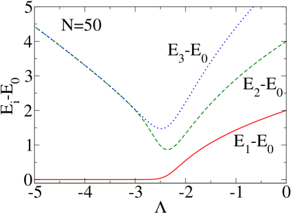
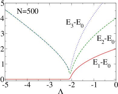
Figure 1: (Color online) Energies of the lowest energy levels with respect to the ground state energy $E_{0}$, as a function of the parameter $\Lambda=NU/J$, for $N=50$ (left panel) and $N=500$ (right panel). All energies are measured in units of $J$.

In principle, one can calculate the matrix elements of the Hamiltonian in the Fock-space basis and by diagonalization obtain the full spectrum of the system and the spectral decomposition of the eigenstates ^{19, 26, 7, 28, 29}. It is then straightforward to calculate also the population imbalance and the degree of condensation of each state.

In this paper we are interested in understanding the physical nature of the ground state of the system, which is for some parameter values quasi-degenerate with the first excited state. Therefore, we start by considering the lowest energy levels of the system as a function of $\Lambda\equiv NU/J$, a parameter governing the behavior of the system. In Fig. 1, we report the energies of the first three excited states with respect to the ground state of the system as a function of $\Lambda$ for two different numbers of particles, $N=50$ and $N=500$, obtained by direct diagonalization ¹⁹. For vanishing atom-atom interaction, $\Lambda=0$, the energy gap for consecutive states is equal (except for the bias), and the gap is independent of the number of particles. As $|\Lambda|$ increases the eigenvalues start to merge in pairs (the ground with the first excited, the second with the third, etc.) but due to both $\varepsilon$ and $J$, they do not reach complete degeneracy. Moreover, the convergence of the merging process depends on the number of particles: for higher $N$ it occurs at smaller values of $|\Lambda|$ reaching the value $|\Lambda|=2$, when the number of particles tends to infinity.

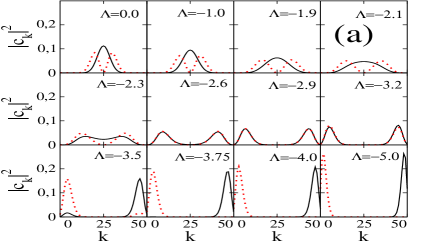
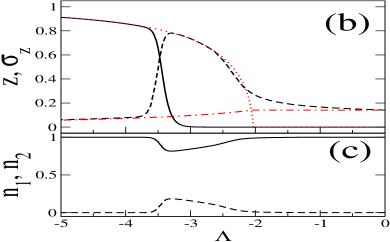
Figure 2: (Color online) (a) Spectral decomposition ($|c_{k}|^{2}$) in the Fock space of the ground (black solid line) and first excited (red dotted line) states for different values of $\Lambda$, with $N=50$. To help in the reading of the figure, instead of plotting the discretized values $|c_{k}|^{2}$ we have generated a smooth curve by joining the different points. (b) Population imbalance $z$ (black solid line) and its dispersion $\sigma_{z}$, Eqs. (4), (black dashed line) of the exact ground state as a function of $\Lambda$. The semi-classical predictions of the imbalance (red dotted line) and its dispersion (red dot-dashed) are also plotted ^{7, 30}. (c) Solid and dotted lines depict the condensed fractions $n_{1}$ and $n_{2}$ of the one-body density matrix of the exact ground state as a function of $\Lambda$. In all cases $N=50$.

In Fig. 2 (a) we plot the spectral decomposition of the ground and first excited states in the Fock space for different values of $\Lambda$, and for $N=50$. The plotted values $|c_{k}|^{2}$ give the probability that the state has $k$ particles in the left well and $N-k$ particles in the right one. Notice that if the spectral decomposition of the state is peaked at high values of $k$, it means that for this state most of the atoms are located on the left side of the double-well. For weak interactions, $|\Lambda|<2.6$, the spectral decomposition of the ground and the first excited states are clearly different, (as were also the energies in Fig. 1). For stronger interactions, $-3.2\leq\Lambda\leq-2.6$, the two states become very close in energy (Fig. 1, left panel) and their spectral decompositions $|c_{k}|^{2}$ are very similar. However, one should notice that the ground state is symmetric, $c_{N/2+k}=c_{N/2-k}$, and the first excited one is antisymmetric, $c_{N/2+k}=-c_{N/2-k}$. In this region the ground state is a strongly correlated cat-like state  as its spectral decomposition has two clear peaks.

Finally, for $|\Lambda|>3.2$, the two states become again clearly different: the ground state is peaked at a high value of $k$, with a large amount of atoms in the left well, while the first excited has its peak at a low value of $k$. Note that the energies of these states are very close to each other.

A useful characterization of the ground state is provided by the population imbalance $z$. As shown in Fig. 2 (b), it remains zero up to a certain value of $|\Lambda|$ ($\sim 3.25$ for $N=50$), approaches 1 as $|\Lambda|$ increases further. The figure also shows $\sigma_{z}$, which starts from small values associated to a relatively narrow binomial distribution. It increases in the range where the strongly cat-like state is present, and finally decreases abruptly when $|\Lambda|$ increases further and the ground state populates massively the $L$ state. Thus $z\rightarrow 1$ and $\sigma_{z}\rightarrow 0$ for $|\Lambda|\rightarrow\infty$.

The degree of condensation of the ground state, $|\phi_{\rm gs}\rangle$, is determined by the eigenvalues $n_{1}$ and $n_{2}$ of the one-body density matrix, which are plotted in Fig. 2 (c). These condensate fractions measure the macroscopic occupations of the single-particle states $|\psi_{1}\rangle$ and $|\psi_{2}\rangle$, eigenfunctions of $\langle\phi_{\rm gs}|\hat{\rho}|\phi_{\rm gs}\rangle$. The regions where these values are not close to 1 and 0, signal the occurrence of fragmentation of the ground state and the impossibility to describe the system by means of a mean-field state. In the region, $-2<\Lambda<0$, $n_{1}$ is rather close to 1 ($n_{1}\sim 0.99$), and the macroscopically occupied state is given by $|\psi_{1}\rangle=(|L\rangle+|R\rangle)/{\sqrt{2}}$, with $|L(R)\rangle\equiv a^{\dagger}_{L(R)}|0\rangle$. However, as we will discuss later in Fig. 3, this slight fragmentation produces noticeable differences in the spectral decomposition of the mean-field state build with the state $|\psi_{1}\rangle$ and the exact ground state. The fragmentation is particularly important for $-2.5>\Lambda>-3.5$, which is roughly the same interval where the cat-like structure takes place. However, the macro-occupied state $|\psi_{1}\rangle$ remains equal to the one previously discussed. The correlations beyond mean-field affect the degree of condensation, but not the single state that is mainly occupied. This is because the ground state remains almost symmetric (except for the bias) in the Fock space (see Fig. 2 (a) and 3), i.e. with $z$ almost zero. This is reflected in the symmetric character of the one-body density matrix, which in turn implies that $|\psi_{1}\rangle$ is the normalized symmetric combination of $|L\rangle$ and $|R\rangle$. For further increasing $|\Lambda|$, the system becomes again condensed: $n_{1}\rightarrow 1$. The slight energy difference introduced by the bias term, which energetically promotes the $|L\rangle$ over the $|R\rangle$ state, drives the system to $|\psi_{1}\rangle\rightarrow|L\rangle$.

The precise value of the bias term has been shown to determine, for a fixed $N$, the size of the cat-like-region. Exploring the interplay between the bias term and the hopping strength, $J$, a good estimate of the precise value of $\Lambda$ where the bias dominates is given in Ref. [30]. For larger number of particles, $N$, the bias term becomes dominant at lower values of $|\Lambda|$ ³⁰, as its effect is proportional to $N$, and therefore the cat-like-region becomes narrower at values of $\Lambda$ closer to the critical classical value $\Lambda=2$.

3 Variational state for the ground state

3.1 Mean-field ansatz

A reliable mean-field state ¹⁹ can be constructed using a general single-particle state $|\phi\rangle_{\rm sp}=\alpha|L\rangle+\beta|R\rangle$, with $|\alpha|^{2}+|\beta|^{2}=1$, and considering all the particles to be in this single-particle state:

$$|\phi\rangle_{N}=\frac{1}{{\sqrt{N!}}}\left[\alpha a_{L}^{\dagger}+\beta a_{R}^{\dagger}\right]^{N}|0\rangle\,.$$ (5)

The expectation value of the Hamiltonian for this state is,

$$E(\alpha,\alpha^{*},\beta,\beta^{*})=\langle\phi|H|\phi\rangle_{N} = -\varepsilon N(\alpha\alpha^{*}-\beta\beta^{*})-JN(\alpha^{*}\beta+\alpha\beta^{*})$$ (6)

$$+\frac{U}{2}N(N-1)(|\alpha|^{4}+|\beta|^{4})\,.$$

The minimization of the energy with respect to the variational parameters, together with the normalization condition $|\alpha|^{2}+|\beta|^{2}=1$, yields the following equation

$$2\varepsilon N-JN\left(\frac{\alpha^{2}-\beta^{2}}{\alpha\beta}\right)+UN(N-1)(|\beta|^{2}-|\alpha|^{2})=0\,.$$ (7)

The possible solutions of the previous equation will be of the type $(\alpha,\pm\beta)$ with both $\alpha$ and $\beta$ positive real numbers. Explicit simple analytic solutions to the previous equation can be obtained by neglecting the bias term. Therefore, taking $\varepsilon=0$ and introducing $\tilde{\Lambda}=\Lambda(N-1)/N$, one gets the following set of solutions ¹⁹:

$$\alpha_{0}=\beta_{0}=\frac{1}{{\sqrt{2}}}\,,\quad\alpha_{\pm}=\beta_{\mp}={\sqrt{\frac{1}{2}\pm{\sqrt{\frac{1}{2^{2}}-\frac{1}{\tilde{\Lambda}^{2}}}}}}\,,$$ (8)

that give rise to the multi-particle states:

$$|\phi_{i}^{\pm}\rangle_{N}=\frac{1}{{\sqrt{N!}}}\left[\alpha_{i}a_{L}^{\dagger}\pm\beta_{i}a_{R}^{\dagger}\right]^{N}|0\rangle\,,$$ (9)

with $i=0,+,-$. Note that the solutions $\alpha_{\pm}$ and $\beta_{\pm}$ only exist when $|\tilde{\Lambda}|>2$. The expectation value of the energy in these states, with $\varepsilon=0$, is :

$$E_{0}^{\pm}\equiv\langle\phi_{0}^{\pm}|H|\phi_{0}^{\pm}\rangle=\frac{U}{4}N(N-1)\mp JN\,,$$ (10)

$$E_{+}^{\pm}\equiv\langle\phi_{+}^{\pm}|H|\phi_{+}^{\pm}\rangle=E_{-}^{\pm}\equiv\langle\phi_{-}^{\pm}|H|\phi_{-}^{\pm}\rangle=\frac{U}{2}N(N-1)-\frac{NJ}{\tilde{\Lambda}}(1\mp 2)\,.$$ (11)

As $U<0$ and $J=1$, the states $|\phi_{i}^{+}\rangle_{N}$ have a lower mean energy than the $|\phi_{i}^{-}\rangle_{N}$ in all cases. To find the lowest energy, we study the difference between $E_{0}^{+}$ and $E_{+}^{+}$ (notice that $E_{+}^{+}=E_{-}^{+}$),

$$E_{0}^{+}-E_{+}^{+}=-NJ\left[\frac{1}{4}\tilde{\Lambda}+\left(\frac{1}{\tilde{\Lambda}}+1\right)\right]\,.$$ (12)

Thus for $|\tilde{\Lambda}|<2$, the lowest energy state is $|\phi_{0}^{+}\rangle_{N}$, and for $\tilde{\Lambda}<-2$, both states $|\phi_{+}^{+}\rangle_{N}$ and $|\phi_{-}^{+}\rangle_{N}$ have the same minimum mean energy.

3.2 Variational ansatz beyond mean-field

In the case that $E_{\pm}^{+}$ are the smallest mean-field energies, i.e., for $|\tilde{\Lambda}|>2$, one can propose an alternative ansatz ¹⁹ for the multi-particle many-body state that goes beyond the mean-field approach and tries to incorporate the cat-like structure :

$$|\phi_{\rm cat}\rangle_{N}={1\over\sqrt{2}}\sqrt{{1\over 1+\big{(}{2/|\tilde{\Lambda}|}\big{)}^{N}}}\Big{(}|\phi_{+}^{+}\rangle_{N}+|\phi_{-}^{+}\rangle_{N}\Big{)}.$$ (13)

The expectation value of the Hamiltonian for this many-body state,

$$\langle\phi_{\rm cat}|H|\phi_{\rm cat}\rangle_{N}={NJ\over 4\tilde{\Lambda}}\Bigg{[}{4-\tilde{\Lambda}^{2}\over 1+(2/|\tilde{\Lambda}|)^{N}}+3\tilde{\Lambda}^{2}\Bigg{]}\,,$$ (14)

is smaller than $E_{\pm}^{+}$. This state is a linear combination of two non-orthogonal mean-field states having the same energy expectation value (if the bias is not taken into account), but two different spectral decompositions. It is precisely the fact that they are not orthogonal that allows the mean energy value in the state $|\phi_{\rm cat}\rangle$ to be smaller than $E_{+}^{+}=E_{-}^{+}$.

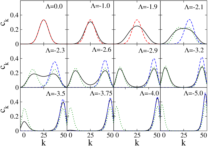
Figure 3: (Color online) Spectral decomposition ($c_{k}$) in Fock space of the ground state of the system, for different values of $\Lambda$, computed by exact diagonalization (black solid line) and compared to the spectral decomposition of the mean-field functions $|\phi_{0}^{+}\rangle_{N}$ for $|\Lambda|<2$ (red dashed line) and $|\phi_{+}^{+}\rangle_{N}$ for $|\Lambda|>2$ (blue dashed line). For $|\Lambda|>2$, we also show the results for the variational cat-state $|\phi_{\rm cat}\rangle$ (green dotted line). In all cases $N=50$.

In Fig. 3, we show the Fock space decomposition ($c_{k}$) for different values of $\tilde{\Lambda}$ of the ground state of the system computed by exact diagonalization of the many-body Hamiltonian, Eq. (1). We compare these coefficients with the ones provided by the mean-field state $|\phi_{0}^{+}\rangle_{N}$ for $|\tilde{\Lambda}|<2$, and $|\phi_{+}^{+}\rangle_{N}$ for $|\tilde{\Lambda}|>2$. In this last case we also plot the results for the variational state $|\phi_{\rm cat}\rangle_{N}$ given in Eq. (13). In all cases $N=50$. Note that for this number of particles $\Lambda$ and $\tilde{\Lambda}$ are very similar and therefore the critical value of $\Lambda$ where the mean-field states $|\phi_{\pm}^{+}\rangle_{N}$ appear is $\Lambda\sim\tilde{\Lambda}=-2$.

For $|\tilde{\Lambda}|<2$, the best mean-field representation of the ground state corresponds to $|\phi_{0}^{+}\rangle_{N}$. The coefficients $c_{k}$ follow a binomial distribution, symmetric around $k=N/2$. This mean-field state gives a good qualitative description of the system in this range, however it coincides with the exact solution only for $\tilde{\Lambda}=0$. In Fig. 3 one can appreciate that the distribution of the exact ground state is slightly broader and the differences increase with $|\tilde{\Lambda}|$ (recall that the fragmentation in this region was very small). The energy difference between $\langle\phi_{0}^{+}|H|\phi_{0}^{+}\rangle$ and the exact ground state energy, $E_{\rm gs}$, relative to $E_{\rm gs}$ is shown in Fig. 4 (a). This relative difference increases with $\Lambda$ and is zero only for $\Lambda=0$. Another measure of the capability of the mean-field state to describe the exact ground state is provided by the overlap of the trial state with the exact ground state. This overlap, $\langle\phi_{\rm gs}|\phi_{0}^{+}\rangle$ is plotted in Fig. 4 (b). The overlap is 1 only for $\Lambda=0$. The differences in the spectral decomposition in the Fock space reflect in an overlap smaller than 1 when $\Lambda$ increases. Clearly at $\Lambda=-2$ the overlap between $\langle\phi_{\rm gs}|\phi_{0}^{+}\rangle$, decreases quickly and tends to zero for large values of $|\Lambda|$.

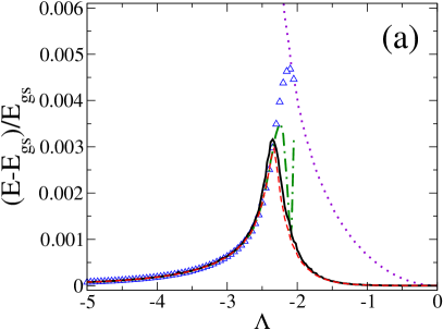
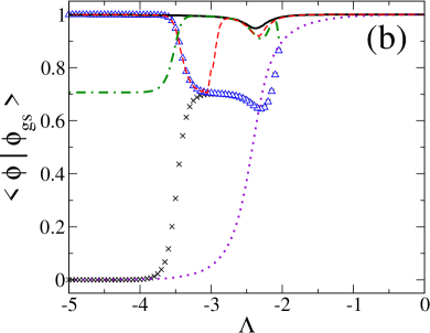
Figure 4: (Color online) (a) Relative difference with respect to the exact ground state energy of the expectation value of the Hamiltonian with different variational many-body states: $|\phi_{0}^{+}\rangle$ (violet dotted line), $|\phi_{\pm}^{+}\rangle$ (blue triangles), $|\phi_{\rm cat}\rangle$ (Eq. 13) (green dot-dashed line), $|\Psi_{\rm var}\rangle_{\rm min}$ (red dashed line) and $|\Psi_{\rm var}\rangle_{\rm max}$, (black solid line). (b) Overlap of the different states discussed in the text with the exact ground state of the system as a function of $\Lambda$. $|\phi_{0}^{+}\rangle$ (violet dotted line), $|\phi_{+}^{+}\rangle$ (blue triangles), $|\phi_{-}^{+}\rangle$(black crosses), $|\phi_{\rm cat}\rangle$ (Eq. 13) (green dot-dashed line), $|\Psi_{\rm var}\rangle_{\rm min}$ (red dashed line) and $|\Psi_{\rm var}\rangle_{\rm max}$ (black solid line).

In the region $-3.2<\tilde{\Lambda}<-2$, the minimum energy mean-field solutions, $|\phi_{+}^{+}\rangle$ and $|\phi_{-}^{+}\rangle$, provide the same energy expectation value when the bias is not taken into account. The Fock decomposition of $|\phi_{+}^{+}\rangle$ is plotted in Fig. 3. The distribution for $|\phi_{-}^{+}\rangle$ would be symmetric with respect to $k=N/2$. The differences of the expectation energies, of these two states ($|\phi_{+}^{+}\rangle$ and $|\phi_{-}^{+}\rangle$), with respect to the ground state energy are rather small, not only in the cat-like state region but also for larger values of $|\Lambda|$, where the difference tends to zero. On the contrary, the behavior of the overlap of these two states with the ground state is rather different. In the cat-state region, both overlaps are rather similar. The reason is that $|\phi_{+}^{+}\rangle$ overlaps with the right part of the cat-state (in the Fock space) and $|\phi_{-}^{+}\rangle$ overlaps with the left part of the cat-state. As $|\Lambda|$ is increased and the cat-state disappears, the presence of the bias term in the Hamiltonian ensures the breaking of the left/right symmetry by energetically promoting the $|L\rangle$ state. Thus, the system selects $|\phi_{+}^{+}\rangle$ as the ground state, and therefore its overlap with the exact ground state tends to 1, while the overlap of $\langle\phi_{\rm gs}|\phi_{-}^{+}\rangle$ tends to zero.

The cat-state structure can be reproduced by defining as trial state the linear combination of $|\phi_{+}^{+}\rangle$ and $|\phi_{-}^{+}\rangle$, Eq. (13), as one can see by looking at the spectral decomposition of this state shown also in Fig. 3. Obviously, when $|\Lambda|$ increases, and the ground state is preferentially located in one of the wells, this state $|\phi_{\rm cat}\rangle$ does not give anymore a good reproduction of the Fock space decomposition of the ground state. If one looks at the overlap $\langle\phi_{\rm gs}|\phi_{\rm cat}\rangle$, this variational state clearly improves the overlap with the ground state in the cat-like region, but when $|\Lambda|$ increases, the overlap tends to a constant ${1/\sqrt{2}}$. The behavior of the energy can be observed in Fig. 4 (a). We can see that there is an improvement in the cat-state region when using $|\phi_{\rm cat}\rangle$. However, when $|\Lambda|$ increases all three functions $|\phi_{\rm cat}\rangle$, $|\phi_{+}^{+}\rangle$ and $|\phi_{-}^{+}\rangle$ become degenerate in energy with the exact ground state.

4 Improved global variational ansatz

We propose a variational ansatz that is valid independent of the strength of the interaction including at the same time the possibility of a mean-field and the existence of a cat-state. This state is a combination of two different mean-field states:

$$|\Psi_{\rm var}\rangle = A|\phi\rangle_{1}+B|\phi\rangle_{2}=\frac{A}{{\sqrt{N!}}}\left[\alpha a_{L}^{\dagger}+\beta a_{R}^{\dagger}\right]^{N}|0\rangle$$ (15)

$$+ \frac{B}{{\sqrt{N!}}}\left[\beta a_{L}^{\dagger}+\alpha a_{R}^{\dagger}\right]^{N}|0\rangle\,.$$

The variational parameters $\alpha$, $\beta$, $A$ and $B$ are taken real. Note that the two mean-field states are not necessarily orthogonal and therefore the normalization conditions are imposed in the following way:

$$\alpha^{2}+\beta^{2}=1\,,\quad A^{2}+B^{2}+2(2\alpha\beta)^{N}AB=1\,.$$ (16)

Let us discuss the differences of the ansatz in Eq. (15) with the states studied in the previous section. Here if $A$ or $B$ are zero, the state reduces to a mean-field state of the type considered before. On the other hand, if one constructs the combination of the two mean-field states and allows for a new minimization of the variational parameters, a noticeable improvement of the state is obtained. The expectation value of the Hamiltonian with this ansatz is given by

$$\frac{E}{JN} = \left[-2\alpha\beta+\frac{\tilde{\Lambda}}{4}(1-4\alpha^{2}\beta^{2})+\frac{1}{2\alpha\beta}\,\right](A^{2}+B^{2})$$ (17)

$$+ \frac{\varepsilon}{J}(\beta^{2}-\alpha^{2})(A^{2}-B^{2})+\frac{\tilde{\Lambda}}{4}-\frac{1}{2\alpha\beta}\,.$$

To determine the parameters of the variational state we follow two different criteria. The first consists in performing a numerical minimization of the expectation value of the energy, Eq. (17). The many-body state thus computed is named $|\Psi_{\rm var}\rangle_{\rm min}$. In the second procedure, which can be pursued only when we already have a numerical solution of the exact ground state, we determine the coefficients by maximizing the overlap of the variational state with the exact ground state, giving the state $|\Psi_{\rm var}\rangle_{\rm max}$.

Figure 5: (Color online) Values of $\alpha$, $\beta$ (a) and of $A$, $B$ (b) obtained in the improved global variational approach of Eq. (15) by overlap maximization (black solid line) and by energy minimization (red dashed line), and the ones obtained in the variational approach of Eq. (13), for which $A=B$ (green dot-dashed line).

The first procedure, which does not require the previous numerical solution of the ground state, produces by construction the closest energy to the exact ground state energy within the form of Eq. (15). As will be discussed in the following, the second criteria although requiring the previous numerical solution of the ground state, produces in all cases an extremely close agreement with the ground state from the energetic point of view, while also improving the overlap with the numerically computed ground state. Thus, for certain applications where an analytical rendition of the state is preferable, our variational proposal should be very useful.

The values of $\alpha,\beta$, $A$, and $B$ obtained in both cases are reported in Fig. 5. For $\Lambda=0$, we have $\alpha=\beta=1/{\sqrt{2}}$ and $A=B=1/2$, recovering the function $|\phi_{0}^{+}\rangle$ that was the exact solution. This is the only case where our improved variational state coincides with the one proposed in Ref. [19]. Obviously in this case both conditions: minimum energy and maximum overlap, provide the same solution. Note that in this case, the overlap between the two components of the generalized variational ansatz ($|\phi\rangle_{1}$ and $|\phi\rangle_{2}$) is maximum, i.e. the two components coincide.

When $|\Lambda|$ is increased, $-2<\Lambda<0$, $\alpha$ and $\beta$ become different while $A$ and $B$ remain equal but different from $1/2$. The improved variational state incorporates correlations beyond mean-field, and the overlaps $\langle\phi_{\rm gs}|\Psi_{\rm var}\rangle_{\rm min}$ and $\langle\phi_{\rm gs}|\Psi_{\rm var}\rangle_{\rm max}$, [see Fig. 4 (b)] clearly improve with respect to $|\phi_{0}^{+}\rangle$. Also the difference in the expectation values of the energies $\langle\Psi_{\rm var}|H|\Psi_{\rm var}\rangle_{\rm min}$ and $\langle\Psi_{\rm var}|H|\Psi_{\rm var}\rangle_{\rm max}$ relative to the ground state energy become smaller as shown in Fig. 4 (a).

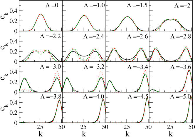
Figure 6: (Color online) Spectral decomposition of the exact ground state (black solid line), and the states obtained using the ansatz defined in Eq. (15) when its overlap with the exact ground state is maximized (green dashed line) or when its energy is minimized (red dotted line).

In this region ($|\Lambda|<2$) the differences between the observables corresponding to these two variational states associated with the maximum overlap or with the minimum energy criteria are rather small. The state that minimizes the energy provides slightly better energies, however this difference is not significant in Fig. 4 (a). Correspondingly the state that maximizes the overlap provides overlaps with the ground state closer to unity. However these differences are also not appreciable in Fig. 4 (b). The Fock decomposition of these two variational states $|\Psi_{\rm var}\rangle_{\rm min}$ and $|\Psi_{\rm var}\rangle_{\rm max}$ compared with the one of the ground state are shown in Fig. 6 for different values of $\Lambda$ and $N=50$. One can observe a clear improvement of the Fock decomposition with respect to the mean-field state in this range of the interaction $|\Lambda|<2$.

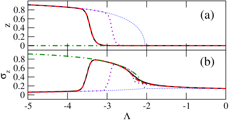
Figure 7: (Color online) (a) Population imbalance $z$ and (b) its dispersion $\sigma_{z}$ as a function of $\Lambda$ for the exact calculation (black solid line), the improved global variational approach in Eq. (15) by overlap maximization (red dashed line) and by energy minimization (violet dotted line) The blue dashed line is the semi-classical prediction and the green dot-dashed line corresponds to the $|\phi_{\rm cat}\rangle_{N}$ of Eq. (13). The number of particles is $N=50$.

Interestingly, the proposed state captures well the correlations beyond mean-field existing in the ground state of the problem before the classical bifurcation. These correlations, as discussed above and shown in Fig. 2 (a), produce very small effects on the condensate fractions but become clearly visible when looking at the spectral decomposition of the ground state, see Fig. 3, or the dispersion of the population imbalance which is no longer corresponding to a simple binomial distribution, see Fig. 2 (b).

Once we cross the classical bifurcation, $\Lambda<-2$, the spectral decomposition of the ground state broadens and at $\Lambda\sim-2.2$ becomes quickly two-peaked. This region where the ground state has two maxima is what we refer to as the cat-state region. The main objective of the variational ansatz introduced in  [19], and discussed in Sect. 3.1, is to describe the ground state properties in this region. The results with the improved global variational ansatz of Eq. (15) are shown in Figs. 4, 6, and 7. Unlike in the region before the bifurcation, here the two criteria used to compute the variational parameters provide fairly different results in some cases. The computed energy of the state is very close with both criteria, but its overlap with the ground state is different depending on the criteria used, see Fig. 4. This is a consequence of the clear differences seen in the spectral decomposition, Fig. 6. The variational solution obtained by minimizing the energy is seen to depart from the exact solution in the region $-3.5<\Lambda<-3$, predicting an earlier transition to the ’self-trapped’ domain, see Figs. 5 and 7.

The criterion of maximizing the overlap implies the ansatz to follow much closer some of the explored ground state properties of the system as shown in Fig. 7, where the agreement with the exact calculation both for the population imbalance and its dispersion is extremely good in the considered domain. Thus, for these parameter values, obtaining a faithful representation of the ground state with the form proposed in Eq. (15) would require the prior numerical solution of the exact ground state.

4.1 Fragmentation of the ground state

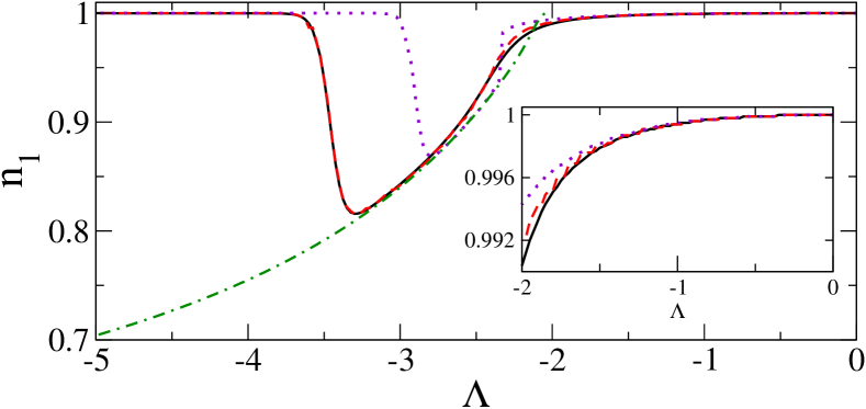
Figure 8: (Color online) Largest eigenvalue of the one body density matrix, $n_{1}$, as a function of $\Lambda$ for the different many-body states discussed in the text: exact calculation (black solid line), $|\Phi_{\rm var}\rangle_{\rm max}$ (red dashed line), $|\Phi_{\rm var}\rangle_{\rm min}$ (violet dotted line), and the cat-state $|\phi_{\rm cat}\rangle$ of Ref. [19] (green dot-dashed line). The inset shows the region before the bifurcation.

To complete the characterization of the proposed states we also study the fragmentation of the ground state of the system. To this end, we calculate the one-body density matrix and look at its larger eigenvalue. If the largest eigenvalue ($n_{1}$) is significantly smaller than unity, we have fragmentation and the system is not condensed in one single state. It also indicates the impossibility to describe the system by a mean-field state and therefore reveals the existence of correlations beyond mean-field. The largest eigenvalue of the one-body density matrix associated to the different states discussed in this work is reported in Fig. 8 for different values of $|\Lambda|$. The two mean-field states, ($|\phi_{0}^{+}\rangle,|\phi_{+}^{+}\rangle$), are not plotted as they have this eigenvalue equal to unity independently of $\Lambda$. The exact ground state gives rise to an $n_{1}$ very close to unity, in the region $|\Lambda|<2$. However, the eigenvalue is strictly one only for $\Lambda=0$, and is actually a smooth decreasing function of $|\Lambda|$. It decreases faster in the cat-like region reaching a minimum ($n_{1}\sim 0.8$) (maximal fragmentation) around $\Lambda=-3.2$. For larger values of $|\Lambda|$ it grows again reaching the value 1 as the system condenses in the left well due to the bias.

The $n_{1}$ associated to the variational state, $|\phi_{\rm cat}\rangle$, which exists for $|\Lambda|>2$, starts from $n_{1}=1$ and decreases with increasing $|\Lambda|$ reproducing rather well the exact $n_{1}$. Contrary to what happens with the exact $n_{1}$, it continues decreasing and increasing the fragmentation failing to reproduce the region dominated by the bias. Finally, the variational many-body states proposed in the present paper, $|\Phi_{\rm var}\rangle_{\rm min}$ and $|\Phi_{\rm var}\rangle_{\rm max}$ reproduce very well the exact $n_{1}$ in the region before the bifurcation, where the system is slightly fragmented, see the inset in Fig. 8. This small fragmentation, as discussed above, indicates the presence of some correlations beyond the mean-field already in this region. In the cat-state region, the $|\Phi_{\rm var}\rangle_{\rm max}$ also reproduces the exact $n_{1}$, see Fig. 8.

5 Conclusions

The variational analytical approach to the two-site Bose-Hubbard model gives a useful insight into the physical nature of the ground state of this apparently simple system that however shows a very rich phenomenology when the interaction or the number of particles change. We have carefully studied the limitations of the mean-field description strongly linked to the presence of fragmentation of the condensate and quantum fluctuations. The proposed variational state is able to describe rather well the exact state and reproduces the energy, the one-body density matrix and thus the fragmentation of the state which are the main magnitudes that we have used to characterize the ground state.

We have also compared the spectral decomposition of the exact ground state with the proposed state obtaining good agreement. The many-body states $|\Phi_{\rm var}\rangle_{\rm min}$, whose parameters are obtained by minimizing the energy, can be used for any number of particles. This state, incorporates for all $\Lambda$s, quantum correlations beyond the mean-field and reproduces very well the fragmentation induced by these correlations which become larger in the cat-state region.

The authors want to thank J. Martorell for a careful reading of the manuscript. M. M.-M. , is supported by an FPI grant from the MICINN (Spain). B.J.-D. is supported by a Grup Consolidat 2009SGR21 contract. This work is also supported by Grants No. FIS2008-01661, and No. 2009SGR1289 from Generalitat de Catalunya.

References

- 1 A. Smerzi, S. Fantoni, S. Giovanazzi, and S.R.Shenoy, Phys. Rev. Lett. 79, 4950 (1997).
- 2 G.J. Milburn, J. Corney, E.M. Wright, and D.F. Walls, Phys. Rev. A 55, 4318 (1997).
- 3 M. Albiez, R. Gati, J. Fölling, S. Hunsmann, M. Cristiani, and M.K. Oberthaler, Phys. Rev. Lett. 95, 010402 (2005).
- 4 S. Ashhab and C. Lobo, Phys. Rev. A 66, 013609 (2002).
- 5 M. Lewenstein, A. Sanpera, V. Ahufinger, B. Damski, A. Sen, and U. Sen, Advances in Physics 56, 243 (2007).
- 6 B. Juliá-Díaz, M. Melé-Messeguer, M. Guilleumas, and A. Polls, Phys. Rev. A 80, 043622 (2009).
- 7 B. Juliá-Díaz, D. Dagnino, M. Lewenstein, J. Martorell, and A. Polls, Phys. Rev. A 81, 023615 (2010).
- 8 B. Juliá-Díaz, J. Martorell, M. Melé-Messeguer, and A. Polls, Phys. Rev. A 82, 063626 (2010).
- 9 M. Abad, M. Guilleumas, R. Mayol, M. Pi, and D.M. Jezek, EPL 94, 10004 (2011).
- 10 C.J. Pethick and H. Smith, Bose-Einstein Condensation in Dilute Gases (Cambridge University Press, 2002).
- 11 L. Pitaevskii and S. Stringari, Bose-Einstein Condensation. (Oxford University Press, Oxford, 2003).
- 12 A. J. Leggett, Rev. Mod. Phys. 73, 307 (2001).
- 13 S. Raghavan, A. Smerzi, S. Fantoni, and S. R. Shenoy, Phys. Rev. A 59, 620 (1999).
- 14 M. Chuchem, K. Smith-Mannschott, M. Hiller, T. Kottos, A. Vardi, and D. Cohen, Phys. Rev. A 82, 053617 (2010).
- 15 T. Zibold, E. Nicklas, C. Gross, and M.K. Oberthaler, Phys. Rev. Lett. 105, 204101 (2010).
- 16 I. Bloch, J. Dalibard, and W. Zwerger, Rev. Mod. Phys. 80, 885 (2008).
- 17 J. Esteve, C. Gross, A. Weller, S. Giovanazzi, and M.K. Oberthaler, Nature 455, 1216 (2008).
- 18 C. Gross, T. Zibold, E. Nicklas, J. Esteve, and M.K. Oberthaler, Nature 464, 1165 (2010).
- 19 J.I. Cirac, M. Lewenstein, K. Mölmer, and P. Zoller, Phys. Rev. A 57, 1208 (1998).
- 20 L.J. Garay, J.R. Anglin, J.I. Cirac, and P. Zoller, Phys. Rev. Lett. 85, 4643 (2000).
- 21 M. Ueda and T. Nakajima, Phys. Rev. A73, 043603 (2006).
- 22 D. Dagnino, N. Barberán, M. Lewenstein, and J. Dalibard, Nature Phys. 5, 431–437 (2009).
- 23 M.I. Parke, N.K. Wilkin, J.M.F. Gunn, and A. Bourne, Phys. Rev. Lett. 101, 110401 (2008).
- 24 A. Nunnenkamp, A.M. Rey, and K. Burnett, Phys. Rev. A 77, 023622 (2008).
- 25 C. Weiss and N. Teichmann, Phys. Rev. Lett. 100, 140408 (2008).
- 26 M. Holthaus and S. Stenholm, Eur. Phys. J. B 20, 451, (2001).
- 27 A. Micheli, D. Jaksch, J. I. Cirac, and P. Zoller, Phys. Rev. A 67, 013607 (2003).
- 28 M.Jääskeläinen and P. Meystre, Phys. Rev. A 71, 043603 (2005).
- 29 V.S. Shchesnovich and M. Trippenbach, Phys. Rev. A 78, 023611 (2008).
- 30 B. Juliá-Díaz, J. Martorell, and A. Polls, Phys. Rev. A 81, 063625 (2010).