Modeling Magnetorotational Turbulence in Protoplanetary Disks with Dead Zones

Abstract

Turbulence driven by magnetorotational instability (MRI) crucially affects the evolution of solid bodies in protoplanetary disks. On the other hand, small dust particles stabilize MRI by capturing ionized gas particles needed for the coupling of the gas and magnetic fields. To provide an empirical basis for modeling the coevolution of dust and MRI, we perform three-dimensional, ohmic-resistive MHD simulations of a vertically stratified shearing box with an MRI-inactive “dead zone” of various sizes and with a net vertical magnetic flux of various strengths. We find that the vertical structure of turbulence is well characterized by the vertical magnetic flux and three critical heights derived from the linear analysis of MRI in a stratified disk. In particular, the turbulent structure depends on the resistivity profile only through the critical heights and is insensitive to the details of the resistivity profile. We discover scaling relations between the amplitudes of various turbulent quantities (velocity dispersion, density fluctuation, vertical diffusion coefficient, and outflow mass flux) and vertically integrated accretion stresses. We also obtain empirical formulae for the integrated accretion stresses as a function of the vertical magnetic flux and the critical heights. These empirical relations allow to predict the vertical turbulent structure of a protoplanetary disk for a given strength of the magnetic flux and a given resistivity profile.

1. Introduction

Planets are believed to form in protoplanetary gas disks. The standard scenario for planet formation consists of the following steps. Initially, submicron-sized dust grains grow into kilometer-sized planetesimals by collisional sticking and/or gravitational instability (Safronov, 1969; Goldreich & Ward, 1973; Weidenschilling & Cuzzi, 1993). Planetesimals undergo further growth toward Moon-sized protoplanets through mutual collision assisted by gravitational interaction (Wetherill & Stewart, 1989). Accretion of the disk gas onto protoplanets leads to the formation of gas giants (Mizuno, 1980; Pollack et al., 1996), while terrestrial planets form through the giant impacts of protoplanets after the gas disk disperses by viscous accretion onto the central star and other effects (Chambers & Wetherill, 1998).

Turbulence in protoplanetary disks plays a decisive role on planet formation as well as on disk dispersal. The impact of turbulence is particularly strong on the formation of planetesimals since the frictional coupling of gas and dust particles governs the process. Classically, planetesimal formation has been attributed to the collapse of a dust sedimentary layer by self-gravity (Safronov, 1969; Goldreich & Ward, 1973) and/or the collisional growth of dust grains (Weidenschilling & Cuzzi, 1993). The presence of strong turbulence is preferable for dust growth when the dust particles is so small that Coulomb repulsion is effective (Okuzumi, 2009; Okuzumi et al., 2011). However, strong turbulence acts against the growth of macroscopic dust aggregates since it makes their collision disruptive (Weidenschilling, 1984; Johansen et al., 2008). Furthermore, turbulence causes the diffusion of a dust sedimentary layer, making planetesimal formation via gravitational instability difficult as well (Weidenschilling, 1984). Turbulence is also known to concentrate dust particles of particular sizes, but its relevance to planetesimal formation via gravitational instability is still under debate (Cuzzi et al., 2001, 2008, 2010; Pan et al., 2011). More recently, it has been suggested that two-fluid instability of gas and dust can produce dust clumps with density high enough for gravitational collapse, but successful dust coagulation to macroscopic sizes seems to be still required for this mechanism to become viable (Youdin & Goodman, 2005; Johansen & Youdin, 2007; Johansen et al., 2007; Bai & Stone, 2010). Besides, turbulence also affects planetesimal growth as turbulent density fluctuations gravitationally interact with planetesimals and can raise their random velocities above the escape velocity (Ida et al., 2008; Nelson & Gressel, 2010). The fluctuating gravitational field can even cause random orbital migration of protoplanets (Laughlin et al., 2004; Nelson & Papaloizou, 2004). Thus, to understand the growth of solid bodies in various stages, it is essential to know the strength and spatial distribution of disk turbulence.

Interestingly, the evolution of solid bodies is not only affected but also affects disk turbulence. The most viable mechanism for generating disk turbulence is the magnetorotational instability (MRI; Balbus & Hawley 1991). This instability has its origin in the interaction between the gas disk and magnetic fields, and therefore requires a sufficiently high ionization degree to operate. Importantly, whether the MRI operates or not in each location of the disk is strongly dependent on the amount of small dust grains because they efficiently capture ionized gas particles and thus reduce the ionization degree (Sano et al., 2000; Ilgner & Nelson, 2006; Okuzumi, 2009). This implies that dust and MRI-driven turbulence affect each other and thus evolve simultaneously.

The purpose of this study is to present an empirical basis for studying the coevolution of solid particles and MRI-driven turbulence. It is computationally intensive to simulate the evolution of dust and MRI-driven turbulence simultaneously, since the evolutionary timescale of solid bodies is generally much longer than the dynamical timescale of the turbulence. For example, turbulent eddies grow and decay on a timescale of one orbital period (e.g., Fromang & Papaloizou, 2006), while dust particles grow to macroscopic sizes and settle to the midplane spending 100–1000 orbital periods (e.g., Nakagawa et al., 1981; Dullemond & Dominik, 2005; Brauer et al., 2008). However, this also means that MRI-driven turbulence can be regarded as quasi-steady in each evolutionary stage of dust evolution. Motivated by this fact, we restrict ourselves to time-independent ohmic resistivity, but instead focus on how the quasi-steady structure of turbulence depends on the vertical profile of the resistivity.

To characterize the vertical structure of MRI-driven turbulence, we perform a number of three-dimensional MHD simulations of local stratified disks including resistivity and nonzero net vertical magnetic flux. Inclusion of a nonzero net vertical flux is important as it determines the saturation level of turbulence (Hawley et al., 1995; Sano et al., 2004; Suzuki & Inutsuka, 2009, see also our Section 4). Similar simulations have been done in a number of previous studies (e.g., Miller & Stone, 2000; Suzuki & Inutsuka, 2009; Oishi & Mac Low, 2009; Suzuki et al., 2010; Turner et al., 2010; Gressel et al., 2011; Simon et al., 2011; Hirose & Turner, 2011). One important difference between our study and previous ones is that we focus on general dependence of the saturated turbulent state on the model parameters such as the resistivity and net magnetic vertical flux.

Our modeling of MRI-driven turbulence follows two steps. In the first step, we seek scaling laws giving the relations among turbulent quantities. We express the relations as a function of the vertically integrated accretion stress, which is the quantity that determines the rate at which turbulent energy is extracted from the differential rotation (Balbus & Papaloizou, 1999). As we will see, excellent scaling relations are obtained if we divide the integrated stress into two components that characterize the contributions from different regions in the stratified disk (which we will call the “disk core” and “atmosphere”) In the second step, we find out empirical formulae that predict the vertically integrated stresses as a function of the resistivity profile and vertical magnetic flux.

The plan of this paper is as follows. In Section 2, we describe the method and setup used in our MHD simulations. In Section 3, we introduce “critical heights” derived from the linear analysis of MRI in stratified disks. As we will see later, these critical heights are useful to characterize the turbulent structure observed in our simulations. We present our simulation results in Section 4, and obtain scaling relations and predictor functions for the quasi-steady state of turbulence in Section 5. In Section 6, we simulate dust settling in a dead zone to model the diffusion coefficient for small particles as a function of height. Effects of numerical resolutions on our simulation results are discussed in Section 7. Our findings are summarized in Section 8.

2. Simulation setup and Method

In this section, we describe the setup and method adopted in our stratified resistive MHD simulations.

2.1. Setup

Our MHD simulations adopt the shearing box approximation (Hawley et al., 1995). We consider a small patch of disk centered on the midplane of an arbitrary distance from the central star, and model it as a stratified shearing box corotating with the angular speed $\Omega$ at the domain center. We use the Cartesian coordinate system $(x,y,z)$, where $x$, $y$, and $z$ stand for the radial, azimuthal, and vertical distance from the domain center. In addition, we assume that the gas is isothermal throughout the box; thus, the sound velocity $c_{s}$ of the gas is constant in both time and space.

2.1.1 Initial Conditions

For the initial condition, we assume that the gas disk is initially in hydrostatic equilibrium and is threaded by uniform vertical magnetic field $B_{z0}$. The assumption of the hydrostatic equilibrium leas to the initial gas density profile

$$\rho=\rho_{0}\exp\left(-\frac{z^{2}}{2h^{2}}\right),$$ (1)

where $\rho_{0}$ is the initial gas density at the midplane and

$$h=\frac{c_{s}}{\Omega}$$ (2)

is the pressure scale height. The ratio between the initial midplane gas pressure $P_{0}=\rho_{0}c_{s}^{2}$ and the initial magnetic pressure $B_{z0}^{2}/8\pi$ defines the initial plasma beta

$$\beta_{z0}\equiv\frac{8\pi\rho_{0}c_{s}^{2}}{B_{z0}^{2}}.$$ (3)

In this paper, the strength of the initial magnetic flux will be referred by $\beta_{z0}^{-1}$ rather than $B_{z0}$.

2.1.2 Resistivity Profile

The main purpose of this study is to see how the turbulence depends on the vertical profile of the ohmic resistivity. We adopt a simple analytic resistivity profile based on the following consideration. For fixed temperature, the resistivity is inversely proportional to the ionization degree (Blaes & Balbus, 1994). In protoplanetary disks, the ionization degree at each location is determined by the balance of ionization (by, e.g., cosmic rays and X-rays) and recombination (in the gas phase and on grain surfaces). Detailed structure of the resistivity profile depends on what processes dominate the ionization and recombination. However, a general tendency is that the ionization degree decreases toward the midplane of the disk, because the ionization rate is lower as the column depth is greater and because the recombination rate is higher as the gas density is higher (see, e.g., Sano et al., 2000). Based on this fact, we give the resistivity profile $\eta(z)$ such that $\eta$ increases as $z$ decreases. To be more specific, we adopt the following resistivity profile

$$\eta=\eta_{\rm mid}\exp\left(-\frac{z^{2}}{2h_{\eta}^{2}}\right),$$ (4)

where $\eta_{\rm mid}$ is the resistivity at the midplane and $h_{\eta}$ is the scale height of $\eta$.

Table 1Model Parameters and Initial Critical Heights

Model	${\displaystyle\frac{\eta_{\rm mid}}{c_{s}h}}$	${\displaystyle\frac{h^{2}}{h_{\eta}^{2}}}$	$\beta_{z0}$	$\log(\Lambda_{0})$	${\displaystyle\frac{h_{{\rm ideal},0}}{h}}$	${\displaystyle\frac{h_{\Lambda,0}}{h}}$	${\displaystyle\frac{h_{{\rm res},0}}{h}}$
Ideal	$0$	$\cdots$	$3\times 10^{5}$	$\infty$	$4.1$	$0.0$	$0.0$
X0	$0.02$	$0.3$	$3\times 10^{5}$	$-3.5$	$4.1$	$3.5$	$2.8$
X1	$0.02$	$1.0$	$3\times 10^{5}$	$-3.5$	$4.1$	$2.8$	$2.2$
X2	$0.02$	$4.0$	$3\times 10^{5}$	$-3.5$	$4.1$	$1.8$	$1.3$
X3	$0.02$	$20.0$	$3\times 10^{5}$	$-3.5$	$4.1$	$0.9$	$0.6$
Y1	$0.0004$	$0.0$	$3\times 10^{5}$	$-1.8$	$4.1$	$2.9$	$0.0$
Y2	$0.0004$	$1.5$	$3\times 10^{5}$	$-1.8$	$4.1$	$1.8$	$0.0$
Y3	$0.0004$	$9.5$	$3\times 10^{5}$	$-1.8$	$4.1$	$0.9$	$0.0$
Y4	$0.0004$	$40.0$	$3\times 10^{5}$	$-1.8$	$4.1$	$0.4$	$0.0$
W1	$1.0$	$2.0$	$3\times 10^{5}$	$-5.2$	$4.1$	$2.8$	$2.4$
W2	$1.0$	$6.4$	$3\times 10^{5}$	$-5.2$	$4.1$	$1.8$	$1.5$
W3	$1.0$	$30.0$	$3\times 10^{5}$	$-5.2$	$4.1$	$0.9$	$0.7$
X1a	$0.02$	$1.0$	$1\times 10^{7}$	$-5.0$	$4.8$	$3.4$	$2.7$
X1b	$0.02$	$1.0$	$3\times 10^{6}$	$-4.5$	$4.6$	$3.2$	$2.5$
X1c	$0.02$	$1.0$	$1\times 10^{5}$	$-3.0$	$3.8$	$2.6$	$1.9$
X1d	$0.02$	$1.0$	$3\times 10^{4}$	$-2.5$	$3.4$	$2.4$	$1.4$
FS03L	$0.01$	$\cdots$	$3\times 10^{5}$	$-3.2$	$4.1$	$1.3$	$0.6$

Equation (4) satisfies the important property of realistic resistivity profiles mentioned above. Furthermore, as shown in Appendix, Equation (4) exactly reproduces the vertical resistivity profile of a disk in some limited cases. However, it will be useful to examine possible influences of limiting $\eta$ to Equation (4). In order to do that, we also consider a resistive profile used in Fleming & Stone (2003),

$$\eta_{\rm FS03}=\eta_{0}\exp\left(-\frac{z^{2}}{4h^{2}}\right)\exp\left(\frac{\Sigma_{0}}{\Sigma_{\rm CR}}\frac{1}{2\sqrt{2\pi}}\int_{|z|/h}^{\infty}e^{-z^{\prime 2}/2}dz^{\prime}\right),$$ (5)

which is characterized by two parameters $\eta_{0}$ and $\Sigma_{0}/\Sigma_{\rm CR}$ (see Equation (10) of Fleming & Stone 2003). Physically, Equation (5) corresponds to the resistivity profile when the ionization degree is determined by the balance between cosmic-ray ionization and gas-phase recombination (see also Appendix).

We construct 17 simulation models using Equations (4) and (5). 16 models are constructed from Equation (4) with various sets of the parameters ($\eta_{\rm mid}$, $h_{\eta}$, $\beta_{z0}$). Table 1 lists the parameters adopted in each run. The model “Ideal” assumes zero resistivity throughout the simulation box. Models X0–X3 are defined by the same value of $\eta_{\rm mid}$ but different values of $h_{\eta}$. The difference between X, Y, and W models is in the value of $\eta_{\rm mid}$. The initial plasma beta is taken to be $3\times 10^{5}$ in all models except X1a–X1d. In addition, we construct one model from Equation (5) with $\eta_{\rm mid}=\eta_{0}\exp(\Sigma_{0}/4\Sigma_{\rm CR})=0.01$ and $\Sigma_{0}/\Sigma_{\rm CR}=34.7$. This set of parameters corresponds to the “larger dead zone” model of Fleming & Stone (2003) defined by ${\rm Re}_{M,{\rm mid}}=100$ and ${\rm Re}_{M,z=2\sqrt{2}h}=5.6\times 10^{6}$, where ${\rm Re}_{M}\equiv c_{s}h/\eta$ is the magnetic Reynolds number with the typical length and velocity set to be $h$ and $c_{s}$, respectively. We refer to the model with these parameters as model FS03L. The initial plasma beta in the FS03L model is taken to be $3\times 10^{5}$. Note that our FS03L run is not exactly the same as the larger dead zone run of Fleming & Stone (2003) since they assumed zero net vertical magnetic flux.

2.2. Method

We solve the equations of the isothermal resistive MHD using the ZEUS code (Stone & Norman, 1992). The domain is a box of size $2\sqrt{2}h\times 8\sqrt{2}h\times 10\sqrt{2}h$ along the radial, azimuthal, and vertical directions, divided into $40\times 80\times 200$ grid cells. For all runs, the radial and azimuthal boundary conditions are taken to be shearing-periodic and periodic, respectively. Therefore, the vertical magnetic flux is a conserved quantity of our simulations. The vertical boundary condition for all runs except X1d is the standard ZEUS outflow condition, where the fields on the boundaries are computed from the extrapolated electromotive forces; only for run X1d, we assume for numerical stability that the magnetic fields are vertical on the top and bottom boundaries as done by Flaig et al. (2010). We have checked that the results hardly depend on the choice of the two types of boundary conditions. Note that the radial and azimuthal components of the mean magnetic fields are not conserved due to the outflow boundary condition. We also added a small artificial resistivity near the boundaries for numerical stability (Hirose et al., 2009). A density floor of $10^{-5}\rho_{0}$ is applied to prevent high Alfvén speeds from halting the calculations.

3. Characteristic Wavelengths and Critical Heights

As we will see in the following sections, it is useful to analyze the simulation results using the knowledge obtained from the linear analysis of MRI. In this subsection, we introduce several quantities that characterize the linear evolution of MRI.

3.1. Characteristic Wavelengths of MRI

According to the local linear analysis of MRI including ohmic resistivity (Sano & Miyama, 1999), the wavelength of the most unstable MRI mode can be approximately expressed as

$$\lambda_{\rm local}\approx\max\{\lambda_{\rm ideal},\lambda_{\rm res}\},$$ (6)

where

$$\lambda_{\rm ideal}\equiv 2\pi\frac{v_{Az}}{\Omega}$$ (7)

and

$$\lambda_{\rm res}\equiv 2\pi\frac{\eta}{v_{Az}}$$ (8)

are the characteristic wavelengths of MRI modes in the ideal and resistive MHD limits, respectively, and $v_{Az}=B_{z}/\sqrt{4\pi\rho}$ is the vertical component of the Alfvén velocity. Equation (6) can be written as $\lambda_{\rm local}\approx\lambda_{\rm ideal}\max\{1,\Lambda^{-1}\}$, where $\Lambda$ is the Elsasser number defined by

$$\Lambda\equiv\frac{v_{Az}^{2}}{\eta\Omega}.$$ (9)

The Elsasser number determines the growth rate of the MRI. If $\Lambda>1$, ohmic diffusion does not affect the most unstable mode lying at $\lambda=\lambda_{\rm ideal}$, and the local instability occurs rapidly at a wavelength $\lambda_{\rm local}\approx\lambda_{\rm ideal}$ and at a rate $\approx\Omega$. If $\Lambda<1$, ohmic diffusion stabilizes the most unstable mode, and the local instability occurs at a longer wavelength $\lambda_{\rm local}\approx\lambda_{\rm res}=\Lambda^{-1}\lambda_{\rm ideal}$ and at a slower rate $\approx\Lambda^{-1}\Omega$. We will refer to the former case as the “ideal MRI,” and to the latter case as the “resistive MRI.”

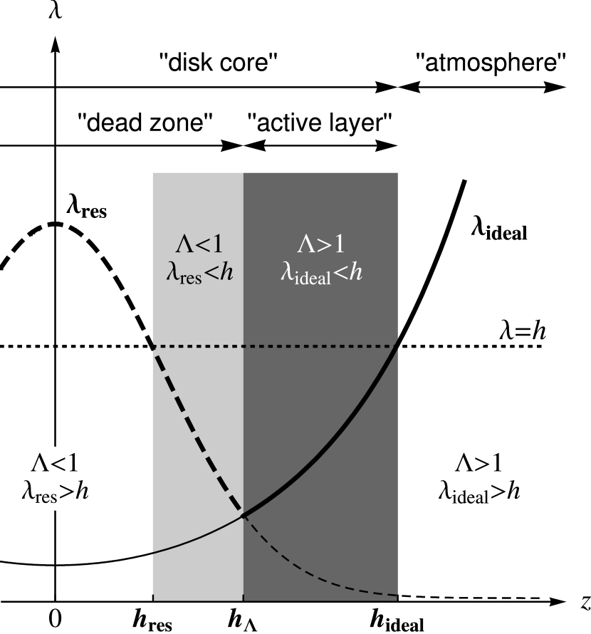
Figure 1.— Schematic illustration showing the vertical structure of a stratified protoplanetary disk with vertical magnetic fields. The horizontal axis shows the distance $z$ from the midplane, while the vertical axis shows the characteristic wavelengths $\lambda_{\rm ideal}$ (solid curve) and $\lambda_{\rm res}$ (dashed curve) of MRI at each $z$ as well as the gas scale height $h$ (dotted line). The set of three ratios $\lambda_{\rm ideal}/h$, $\lambda_{\rm res}/h$, and $\lambda_{\rm ideal}/\lambda_{\rm res}\equiv\Lambda$ defines four layers. At $|z|>h_{\rm ideal}$ ($\Lambda>1$ and $\lambda_{\rm ideal}>h$), MRI is stabilized due to the weak gas pressure compared to the magnetic tension. At $h_{\Lambda}<|z|<h_{\rm ideal}$ ($\Lambda>1$ and $\lambda_{\rm ideal}<h$; dark gray region), MRI operates without affected by ohmic dissipation. At $h_{\rm res}<|z|<h_{\Lambda}$ ($\Lambda<1$ and $\lambda_{\rm res}<h$; light gray region), ohmic dissipation is effective and MRI operates only weakly. At $|z|<h_{\rm res}$ ($\Lambda<1$ and $\lambda_{\rm res}>h$), ohmic dissipation perfectly stabilizes MRI. We refer to the regions $|z|<h_{\rm ideal}$ and $|z|>h_{\rm ideal}$ as the “disk core” and “atmosphere,” respectively.

Figure 1 schematically illustrates how $\lambda_{\rm ideal}$ and $\lambda_{\rm res}$ vary with height $|z|$. In general, $\lambda_{\rm ideal}$ grows toward higher $|z|$ because the Alfvén speed $v_{Az}$ increases as the density decreases. By contrast, $\lambda_{\rm res}$ grows toward lower $|z|$ because $\lambda_{\rm res}$ is inversely proportional to $v_{Az}$ and because $\eta$ increases with decreasing $|z|$ (see the discussion in Section 2.1.2).

The global instability of a stratified disk can be described in terms of the local analysis. As shown by Sano & Miyama (1999), the gas motion at height $z$ is unstable if the local unstable wavelength $\lambda_{\rm local}$ is shorter than the scale height of the disk, i.e.,

$$\max\{\lambda_{\rm ideal},\lambda_{\rm res}\}\lesssim h.$$ (10)

3.2. Critical Heights

With the global instability criterion (Equation (10)) together with the vertical dependence of $\lambda_{\rm ideal}$ and $\lambda_{\rm res}$, we can define three different critical heights for a stratified disk.

1. The first one is $h_{\rm ideal}$ defined by

   $$\lambda_{\rm ideal}({z=h_{\rm ideal}})=h,$$ (11)

   or equivalently, $\beta_{z}(z=h_{\rm ideal})=8\pi^{2}$, where $\beta_{z}(z)=8\pi\rho(z)c_{s}^{2}/B_{z}^{2}(z)$. At $|z|\gtrsim h_{\rm ideal}$ ($\beta_{z}\lesssim 8\pi^{2}$), MRI does not operate because the wavelengths of the unstable modes exceed the disk thickness $\sim h$ (Sano & Miyama, 1999). We refer to the region $|z|\geqslant h_{\rm ideal}$ as the “atmosphere” and to the region $|z|\leqslant h_{\rm ideal}$ as the “disk core.”

2. The second one is $h_{\Lambda}$ defined by

   $$\Lambda(z={h_{\Lambda}})=1,$$ (12)

   or equivalently, $\lambda_{\rm ideal}(z={h_{\Lambda}})=\lambda_{\rm res}(z={h_{\Lambda}})$. The layer $h_{\Lambda}\leqslant|z|\leqslant h_{\rm ideal}$ is the so-called “active layer,” where MRI operates without affected by ohmic diffusion nor gas stratification. The region $|z|\leqslant h_{\Lambda}$ is what we call the “dead zone,” where ohmic diffusion stabilizes the most unstable ideal MRI mode. For convenience, we regard $h_{\Lambda}$ as zero when a dead zone is absent. This is the case for model Ideal.

3. The third one is $h_{\rm res}$ defined by

   $$\lambda_{\rm res}({z=h_{\rm res}})=h.$$ (13)

   Ohmic diffusion allows the resistive MRI to operate at $h_{\rm res}\lesssim|z|\lesssim h_{\Lambda}$. At $|z|\lesssim h_{\rm res}$, ohmic diffusion stabilizes all the unstable MRI modes. Note that some previous studies (e.g., Gammie, 1996; Sano et al., 2000) used the terminology “dead zone” for the region $|z|\leqslant h_{\rm res}$ rather than $|z|\leqslant h_{\Lambda}$. In fact, as we will see in Section 4, the set of $h_{\Lambda}$ and $h_{\rm res}$ best characterizes our dead zone. We regard $h_{\rm res}$ as zero when $\lambda_{\rm res}$ is less than $h$ at all heights. This is the case for Y models.

The critical heights in the initial state ($h_{{\rm ideal},0}$, $h_{\Lambda,0}$, and $h_{{\rm res},0}$) are shown in Table 1 for all of our 17 simulations. Using Equations (1) and (4), one can analytically calculate the initial critical heights for models except FL03L as

$$h_{{\rm ideal},0}=\left[2\ln\biggl{(}{\displaystyle\frac{\beta_{z0}}{8\pi^{2}}}\biggr{)}\right]^{1/2}h,$$ (14)

$$h_{\Lambda,0}=\left(\frac{2\ln\Lambda_{0}^{-1}}{1+(h/h_{\eta})^{2}}\right)^{1/2}h,$$ (15)

$$h_{{\rm res},0}=\Biggl{[}{\displaystyle\frac{2\ln\left(8\pi^{2}\beta_{z0}^{-1}\Lambda_{0}^{-2}\right)}{1+2(h/h_{\eta})^{2}}}\Biggr{]}^{1/2}h,$$ (16)

where

$$\Lambda_{0}=\frac{2c_{s}h}{\eta_{\rm mid}\beta_{z0}}$$ (17)

is the initial Elsasser number at the midplane.

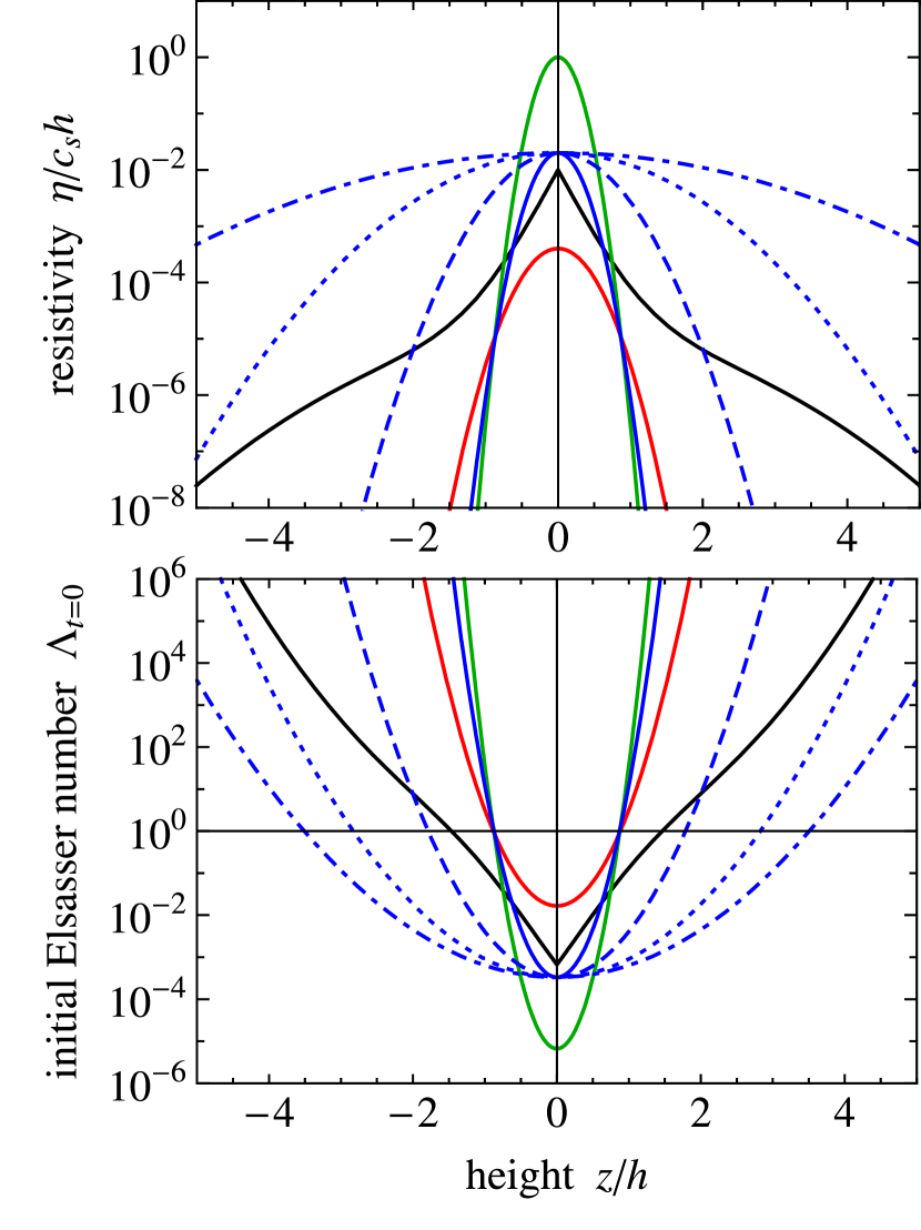
Figure 2.— Vertical profiles of the ohmic resistivity $\eta$ (upper panel) and the initial Elsasser number $\Lambda_{t=0}$ (lower panel) for models X0 (blue dot-dashed curve), X1 (blue dotted curve), X2 (blue dashed curve), X3 (blue solid curve), Y3 (red curve), W3 (green curve), and FS03L (black curve).

Figure 2 shows the vertical profiles of the resistivity $\eta$ and the initial Elsasser number $\Lambda_{t=0}$ for some of our models. The initial midplane Elsasser number $\Lambda_{0}$ and initial critical heights ($h_{{\rm ideal},0},h_{\Lambda,0},h_{{\rm res},0}$) are listed in Table 1 for all models. As one can see from Table 1 and the lower panel of Figure 2, models labeled by the same number are arranged so that they have similar values of $h_{\Lambda,0}$.

For turbulent states, we evaluate $v_{Az}$ in the Elsasser number and the characteristic wavelengths as $({\overline{B_{z}^{2}}}/4\pi{\overline{\rho}})^{1/2}$, where the overbars denote the horizontal averages.

4. Simulation Results

4.1. The Fiducial Model

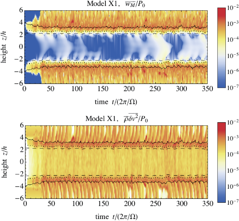
Figure 3.— Horizontally averaged Maxwell stress ${\overline{w_{M}}}$ (upper panel) and density-weighted velocity dispersion ${\overline{\rho}}{\overline{\delta v^{2}}}$ (bottom panel) as a function of time $t$ and height $z$ for model X1. The solid, dotted, and dashed lines show the critical heights $z=h_{\rm ideal}$, $h_{\Lambda}$, and $h_{\rm res}$, respectively.

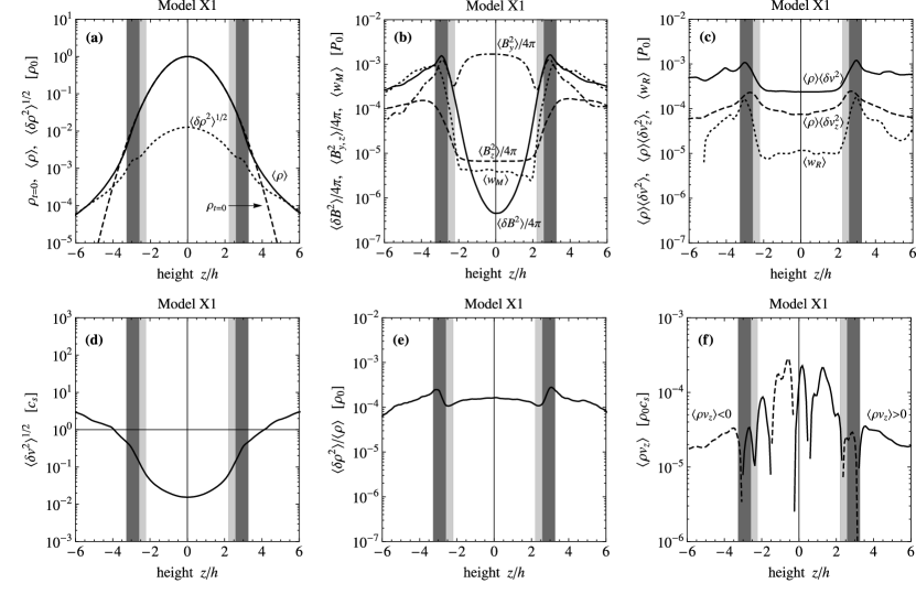
Figure 4.— Vertical profiles of various quantities averaged over $x$–$y$ planes and over a time interval $175~{}{\rm orbits}<t<350~{}{\rm orbits}$ for model X1. (a) Initial (dashed curve) and time-averaged (solid curve) gas densities, and amplitude of the density fluctuation (dotted curve). (b) Magnetic energies $\langle\delta B^{2}\rangle/4\pi$ (solid curve), $\langle B_{y}^{2}\rangle/4\pi$ (dot-dashed curve), and $\langle B_{z}^{2}\rangle/4\pi$ (dashed curve), and Maxwell stress $\langle w_{M}\rangle$ (dotted curve) normalized by the initial midplane gas pressure $P_{0}=\rho_{0}c_{s}^{2}$. (c) Density-weighted velocity dispersions $\langle\rho\rangle\langle\delta v^{2}\rangle$ (thick solid curve) and $\langle\rho\rangle\langle\delta v_{z}^{2}\rangle$ (dashed curve), and Reynolds stress $\langle w_{R}\rangle$ (dotted curve). (d) Root-mean-squared random velocity $\langle\delta v^{2}\rangle^{1/2}$. (e) $\langle\delta\rho^{2}\rangle/\langle\rho\rangle$, which represents the thermal energy of fluctuation. (f) Vertical mass flux $\langle\rho v_{z}\rangle$, plotted for positive (solid curve) and negative (dashed curve) values. The regions shaded in dark and light gray indicate where ideal and resistive MRIs operate, respectively (see also Figure 1).

We select model X1 as the fiducial model to describe in detail. Figure 3 shows how MRI-driven turbulence reaches a quasi-steady state in run X1. The upper and lower panels plot the horizontal averages of the Maxwell stress ${\overline{w_{M}}}=-{\overline{\delta B_{x}\delta B_{y}}}/4\pi$ and the density-weighted velocity dispersion ${\overline{\rho}}{\overline{\delta v^{2}}}$, respectively, as a function of time $t$ and height $z$. The solid, dotted, and dashed lines are the loci of the critical heights $h_{\rm ideal}$, $h_{\Lambda}$, and $h_{\rm res}$, respectively. As seen in the figure, a quasi-steady state is reached within the first 40 orbits. The critical height $h_{\rm ideal}$ measured in the quasi-steady state is slightly lower than that in the initial nonturbulent state. This is because the ideal MRI wavelength $\lambda_{\rm ideal}\propto v_{Az}$ is increased by the fluctuation in the vertical magnetic field, $\delta B_{z}^{2}$. By contrast, $h_{\Lambda}$ and $h_{\rm res}$ are almost unchanged, because the fluctuation of the magnetic field is suppressed in the dead zone.

Figure 4 shows the vertical structure of the disk averaged over a time interval $175<\Omega t/(2\pi)<350$. The dark and light gray bars in each panel indicate the heights where ideal and resistive MRIs operate, respectively (see also Figure 1). The brackets $\langle\cdots\rangle$ denote the averages over time and horizontal directions.

In Figure 4(a), we compare the averaged gas density $\langle\rho\rangle$ with the initial density given by Equation (1). We see that the density is almost unchanged in the disk core ($|z|<h_{\rm ideal}$) but is considerably increased in the atmosphere ($|z|>h_{\rm ideal}$). This is because the magnetic pressure is negligibly small in the disk core but dominates over the gas pressure in the atmosphere. Figure 4(a) also shows the amplitude of the density fluctuation, $\langle\delta\rho^{2}\rangle^{1/2}$. As one can see, the density fluctuation is small ($\langle\delta\rho^{2}\rangle^{1/2}\ll\langle\rho\rangle$) except at $|z|\gg h_{\rm ideal}$.

The magnetic activity in the disk can be seen in Figure 4(b), where the vertical profiles of the magnetic energies ($\langle\delta B^{2}\rangle/4\pi$, $\langle B_{y}^{2}\rangle/4\pi$, and $\langle B_{z}^{2}\rangle/4\pi$) and Maxwell stress $\langle w_{M}\rangle$ are plotted. One can see that these quantities peak near the outer boundaries of the active layers, $|z|\approx h_{\rm ideal}$. This is because the largest channel flows develop at locations where $\lambda_{\rm ideal}\approx h$ (see, e.g., Suzuki & Inutsuka, 2009). In the dead zone, ohmic dissipation suppresses the fluctuation in the magnetic fields, $\langle\delta B^{2}\rangle$, leaving the initial vertical field ($\langle B_{z}^{2}\rangle\approx B_{z0}^{2}$) and coherent toroidal fields ($\langle B_{y}^{2}\rangle\approx\langle B_{y}\rangle^{2}$) generated by the differential rotation.

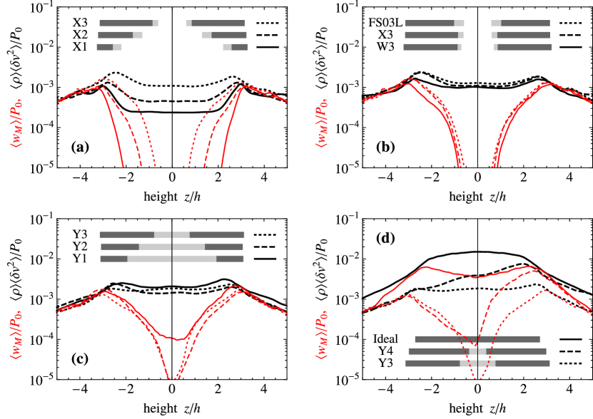
Figure 5.— Vertical profiles of temporally and horizontally averaged Maxwell stress $\langle w_{M}\rangle$ (red curves) and density-weighted velocity dispersion $\langle\rho\rangle\langle\delta v^{2}\rangle$ (black curves) normalized by the initial midplane gas pressure $P_{0}=\rho_{0}c_{s}^{2}$ for $\beta_{z0}=3\times 10^{5}$ models. The dark gray bars indicate where MRI operates without affected by ohmic resistivity ($h_{\Lambda}<|z|<h_{\rm ideal}$), while the light gray bars show where MRI operates but is weakened by ohmic resistivity ($h_{\rm res}<|z|<h_{\Lambda}$).

Figure 4(c) shows the density-weighted velocity dispersions $\langle\rho\rangle\langle\delta v^{2}\rangle$ and $\langle\rho\rangle\langle\delta v_{z}^{2}\rangle$ and the Reynolds stress $\langle w_{R}\rangle=\langle\rho\delta v_{x}\delta v_{y}\rangle$. These quantities characterize the kinetic energy in the random motion of the gas. Comparing Figures 4(b) and (c), we find that the drop in these quantities in the disk core is not as significant as the drop in $\langle\delta B^{2}\rangle$ and $\langle w_{M}\rangle$. This is an indication that sound waves generated in the active layers penetrate deep inside the dead zone (Fleming & Stone, 2003). Furthermore, we find that $\langle\rho\rangle\langle\delta v^{2}\rangle$ is approximately constant, i.e., the velocity dispersion $\langle\delta v^{2}\rangle$ is inversely proportional to the mean density $\langle\rho\rangle$, in the disk core. This means that the kinetic energy density of fluctuation is nearly constant in the disk core. This is another indication of sound waves, because the amplitude of the velocity fluctuation $\delta v$ is generally proportional to $1/\sqrt{\rho}$ for freely propagating sound waves. The root-mean-squared random velocity $\langle\delta v^{2}\rangle^{1/2}$ is shown in Figure 4(d). The random velocity is subsonic in the disk core and exceeds the sound speed only in the atmosphere.

An indication of freely sound waves can be also found in the density fluctuation. Shown in Figure 4(e) is the mean squared density fluctuation $\langle\delta\rho^{2}\rangle$ divided by the mean density $\langle\rho\rangle$. Since $\langle\delta\rho^{2}\rangle^{1/2}\ll\langle\rho\rangle$, the quantity $\langle\delta\rho^{2}\rangle/\langle\rho\rangle\approx\langle\delta\rho^{2}/\rho\rangle$ is approximately proportional to the thermal energy density of fluctuation, $\langle c_{s}^{2}\delta\rho^{2}/2\rho\rangle$. In the disk core, we see that $\langle\delta\rho^{2}\rangle/\langle\rho\rangle$ is roughly constant along the vertical direction, meaning that the amplitude of the density fluctuation, $\langle\delta\rho^{2}\rangle^{1/2}$, is proportional to the square root of the mean density $\langle\rho\rangle$. The similarity between $\langle\rho\rangle\langle\delta v^{2}\rangle$ and $\langle\delta\rho^{2}\rangle/\langle\rho\rangle$ is peculiar to sound waves, for which $\delta v/c_{s}\sim\delta\rho/\rho$.

Figure 4(f) displays the profile of the vertical mass flux $\langle\rho v_{z}\rangle$. In the atmosphere, the vertical flux is outward, i.e., $\langle\rho v_{z}\rangle>0$ at $z>h_{\rm ideal}$ and $\langle\rho v_{z}\rangle<0$ at $z<-h_{\rm ideal}$. This outflow results from the breakup of large channel flows at the outer boundaries of the active layers, $|z|\approx h_{\rm ideal}$ (Suzuki & Inutsuka, 2009; Suzuki et al., 2010). The vertical mass flux reaches a constant value at $|z|\gtrsim 5h$. This fact allows us to measure a well-defined outflow flux for each simulation (see Section 5.1.3).

4.2. Model Comparison

We now investigate how the vertical structure of turbulence depends on the resistivity profile and vertical magnetic flux.

Figure 5 displays the temporal and horizontal averages of the Maxwell stress $\langle w_{M}\rangle$ and the density-weighted velocity dispersion $\langle\rho\rangle\langle\delta v^{2}\rangle$ as a function of $z$ for various $\beta_{z0}=3\times 10^{5}$ models. As in Figures 1 and 4, the dark and light gray bars in each panel indicate the heights where ideal and resistive MRIs operate, respectively.

The effect of changing the size of the dead zone can be seen in Figure 5(a), where models X1, X2, and X3 are compared. These models are characterized by the same values of $\beta_{z0}$ and $\Lambda_{0}$ but different values of $h_{\eta}$. For all the models, $\langle w_{M}\rangle$ sharply falls at $z\sim h_{\rm res}$, meaning that $h_{\rm res}$ well predicts where the resistivity shuts off the magnetic activity. By contrast, $\langle\rho\rangle\langle\delta v^{2}\rangle$ exhibits a flat profile at $|z|\lesssim h_{\rm ideal}$ with no distinct change across $z=h_{\rm res}$ nor $z=h_{\Lambda}$. The only clear difference is the value of $\langle\rho\rangle\langle\delta v^{2}\rangle$ in the disk core, i.e., the value is lower when the dead zone is wider. Note that $\langle\rho\rangle\langle\delta v^{2}\rangle$ decreases more slowly than the column density of the active layers $(h_{\Lambda}<|z|<h_{\rm ideal})$. For example, the active column density in model X1 is 20 times smaller than that in model X3. However, the midplane value of $\langle\rho\rangle\langle\delta v^{2}\rangle$ in the former is only five times smaller than that in the latter. This suggests that even a very thin active layer can provide a large velocity dispersion near the midplane.

Interestingly, the vertical structure of turbulence depends on the critical heights ($h_{\rm ideal}$, $h_{\Lambda}$, and $h_{\rm res}$) but are very insensitive to the details of the resistivity profile. This can be seen in Figure 5(b), where we compare runs with similar critical heights (runs X3, W3, and FS03L). We see that these models produce very similar vertical profiles of $\langle w_{M}\rangle$ and $\langle\rho\rangle\langle\delta v^{2}\rangle$ even though they assume quite different resistivity profiles (see the upper panel of Figure 2). This suggests that the vertical structure of turbulence is determined by the values of the critical heights.

Importance of distinguishing $h_{\Lambda}$ and $h_{\rm res}$ is illustrated in Figures 5(c) and (d). These panels compare five models (Y1–4 and Ideal) in which the resistive MRI is active at the midplane, i.e., $h_{\rm res}=0$. Figure 5(c) shows models with $h_{\Lambda}>0.5h$. We see that the profiles of $\langle\rho\rangle\langle\delta v^{2}\rangle$ and $\langle w_{M}\rangle$ are very similar for the three models. This implies that the vertical structure is determined by the value of $h_{\rm res}$ when $h_{\Lambda}\gtrsim 0.5h$. Figure 5(d) shows what happens when $h_{\Lambda}$ falls below $0.5h$. Model Ideal is clearly different from the other models. Model Y4 ($h_{\Lambda}=0.4$) is interesting because it exhibits both features. In the lower half of the disk ($z<0$), the Maxwell stress behaves as in the other Y models. In the upper half ($z>0$), however, the profile of $\langle w_{M}\rangle$ is closer to that in model Ideal.

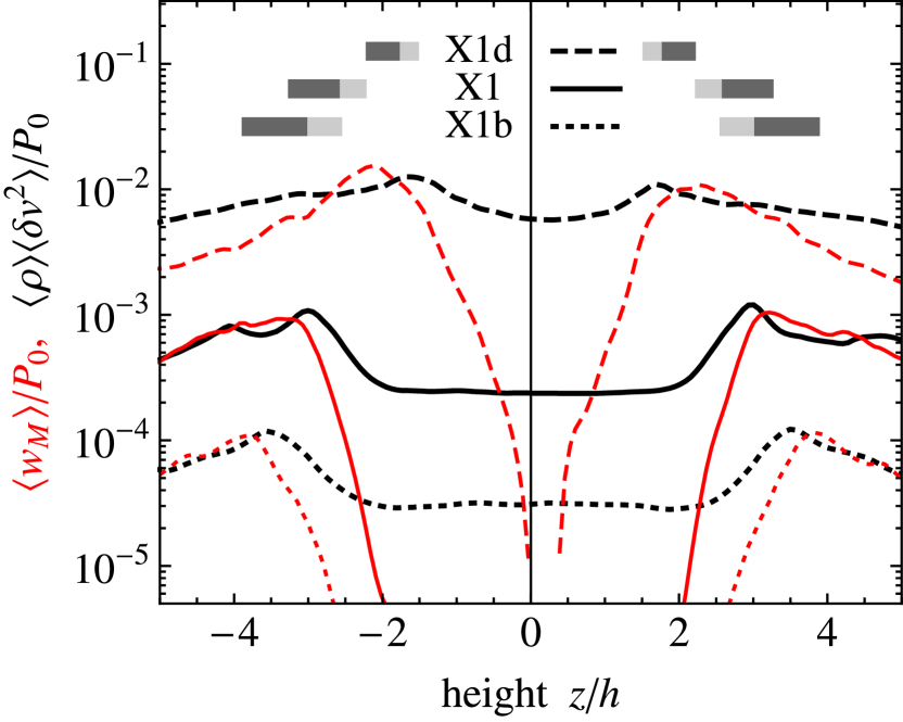
Figure 6.— Vertical profiles of temporally and horizontally averaged Maxwell stress $\langle w_{M}\rangle$ (red curves) and density-weighted velocity dispersion $\langle\rho\rangle\langle\delta v^{2}\rangle$ (black curves) for models with different $\beta_{z0}$. The dotted, solid, and dashed curves correspond to models X1b, X1, and X1d, respectively.

Next, we see how the saturation level of turbulence depends on the vertical magnetic flux. Figure 6 shows the vertical profiles of $\langle w_{M}\rangle$ and $\langle\rho\rangle\langle\delta v^{2}\rangle$ for three runs with different values of $\beta_{z0}$ (X1b, X1, and X1d). We see that these values increase with decreasing $\beta_{z0}$. The peak value of $\langle w_{M}\rangle$ is approximately $10^{-4}P_{0}$, $10^{-3}P_{0}$, and $10^{-2}P_{0}$ for runs X1b, X1, and X1d, respectively ($P_{0}=\rho_{0}c_{s}^{2}$ is the initial midplane gas pressure). This indicates a linear scaling between the turbulent stress and $\beta_{z0}^{-1}$.

5. Scaling Relations and Predictor Functions

Now we seek how the amplitudes of turbulent quantities depend on the vertical magnetic flux and the resistivity profile. We do this in two steps. First, we derive relations between the amplitudes of turbulent quantities and the vertically integrated turbulent stress. We then obtain empirical formulae that predict the integrated stress as a function of the vertical magnetic flux and the resistivity profile.

5.1. Scaling Relations between Turbulent Quantities and Vertically Integrated Accretion Stresses

The ultimate source of the energy of turbulence is the shear motion of the background flow. The accretion stress $w_{xy}\equiv w_{R}+w_{M}$ determines the rate at which the free energy is extracted. Therefore, we expect that the accretion stress is related to the amplitudes of turbulent quantities, such as the gas velocity dispersion and outflow mass flux.

To quantify the rate of the energy input in the simulation box, we introduce the effective $\alpha$ parameter

$$\alpha\equiv\frac{\int\langle w_{xy}\rangle dz}{\Sigma c_{s}^{2}},$$ (18)

where $\Sigma=\int\langle\rho\rangle dz$ is the gas surface density. In the classical, one-dimensional viscous disk theory (Lynden-Bell & Pringle, 1974), the parameter $\alpha$ is related to the turbulent viscosity $\nu_{\rm trub}$ as $\nu_{\rm trub}=(3/2)\alpha c_{s}^{2}/\Omega$, where the prefactor $3/2$ comes from the slope of the Keplerian rotation. Thus, $\alpha$ also characterizes the vertically integrated mass accretion rate.

As we will see below, it is useful to decompose $\alpha$ as $\alpha=\alpha_{\rm core}+\alpha_{\rm atm}$, where

$$\alpha_{\rm core}\equiv\frac{\int_{|z|<h_{\rm ideal}}\langle w_{xy}\rangle dz}{\Sigma c_{s}^{2}}$$ (19)

and

$$\alpha_{\rm atm}\equiv\frac{\int_{|z|>h_{\rm ideal}}\langle w_{xy}\rangle dz}{\Sigma c_{s}^{2}}$$ (20)

are the contributions from the disk core ($|z|<h_{\rm ideal}$) and atmosphere ($|z|>h_{\rm ideal}$), respectively. Table 2 shows the values of $\alpha$, $\alpha_{\rm core}$, and $\alpha_{\rm atm}$ as well as the time-averaged critical heights ($h_{\rm ideal}$, $h_{\Lambda}$, $h_{\rm res}$) for all our simulations.

Table 2Time-averaged Properties of MHD Simulations

Model	${\displaystyle\frac{h_{{\rm ideal}}}{h}}$	${\displaystyle\frac{h_{\Lambda}}{h}}$	${\displaystyle\frac{h_{{\rm res}}}{h}}$	${\displaystyle\frac{\alpha}{10^{-3}}}$	${\displaystyle\frac{\alpha_{\rm core}}{10^{-3}}}$	${\displaystyle\frac{\alpha_{\rm atm}}{10^{-3}}}$	${\displaystyle\frac{\langle\delta v^{2}\rangle_{\rm mid}}{10^{-3}c_{s}^{2}}}$	${\displaystyle\frac{\langle\delta v_{z}^{2}\rangle_{\rm mid}}{\langle\delta v^{2}\rangle_{\rm mid}}}$	${\displaystyle\frac{\langle\delta\rho^{2}\rangle_{\rm mid}}{10^{-3}\langle\rho\rangle_{\rm mid}^{2}}}$	${\displaystyle\frac{\dot{m}_{w}}{10^{-5}\langle\rho\rangle_{\rm mid}c_{s}^{2}}}$
Ideal	$2.4$	$0.0$	$0.0$	$18$	$12$	$6.0$	$15$	$0.22$	$6.4$	$4.7$
X0	$3.3$	$3.0$	$2.8$	$1.9$	$0.30$	$1.6$	$0.13$	$0.34$	$0.12$	$2.5$
X1	$3.2$	$2.5$	$2.2$	$2.0$	$0.42$	$1.5$	$0.24$	$0.32$	$0.16$	$2.8$
X2	$3.1$	$1.7$	$1.3$	$2.3$	$0.68$	$1.6$	$0.45$	$0.35$	$0.27$	$2.9$
X3	$3.0$	$0.8$	$0.6$	$3.3$	$1.4$	$1.9$	$1.1$	$0.32$	$0.66$	$2.9$
Y1	$2.9$	$1.6$	$0.0$	$4.3$	$2.0$	$2.2$	$2.1$	$0.26$	$1.2$	$3.4$
Y2	$3.0$	$1.3$	$0.0$	$3.6$	$1.5$	$2.1$	$1.4$	$0.31$	$0.84$	$3.4$
Y3	$3.0$	$0.8$	$0.0$	$3.5$	$1.6$	$1.9$	$1.8$	$0.23$	$1.2$	$3.0$
Y4	$2.8$	$0.4$	$0.0$	$7.0$	$3.8$	$3.3$	$3.9$	$0.26$	$2.2$	$4.0$
W1	$3.2$	$2.6$	$2.4$	$1.9$	$0.37$	$1.5$	$0.24$	$0.36$	$0.16$	$3.1$
W2	$3.2$	$1.7$	$1.5$	$2.1$	$0.59$	$1.5$	$0.38$	$0.37$	$0.23$	$2.6$
W3	$3.1$	$0.9$	$0.7$	$2.7$	$1.1$	$1.7$	$1.0$	$0.39$	$0.51$	$2.7$
X1a	$4.2$	$3.2$	$2.7$	$0.061$	$0.014$	$0.047$	$0.0097$	$0.17$	$0.0083$	$0.049$
X1b	$3.8$	$2.9$	$2.5$	$0.19$	$0.056$	$0.13$	$0.031$	$0.25$	$0.023$	$0.29$
X1c	$2.8$	$2.2$	$1.9$	$7.6$	$1.4$	$6.2$	$0.93$	$0.40$	$0.50$	$9.0$
X1d	$2.0$	$1.6$	$1.4$	$29$	$8.0$	$21$	$7.0$	$0.47$	$1.8$	$59$
FS03L	$3.0$	$1.0$	$0.6$	$3.4$	$1.5$	$2.0$	$1.3$	$0.35$	$0.70$	$3.1$

5.1.1 Velocity Dispersion

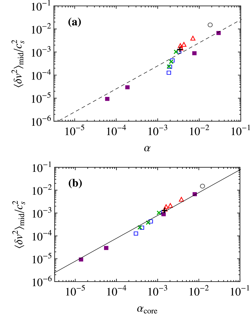
Figure 7.— Gas velocity dispersion at the midplane, $\langle\delta v^{2}\rangle_{\rm mid}$, for all runs presented in this study. Panels (a) and (b) plot the data versus $\alpha$ and $\alpha_{\rm core}$, respectively. The symbols correspond to models Ideal (circle), X0–X3 (open squares), Y1–Y4 (triangles), W1–W3 (crosses), X1a–X1d (filled squares), and FS03L (plus sign). The lines show the best linear fits (Equation (21) for panel (b)).

Random motion of the gas crucially affects the growth of dust particles as it enhances the collision velocity between the particles via friction forces (Weidenschilling, 1984; Johansen et al., 2008). Here, we seek how the velocity dispersion $\langle\delta v^{2}\rangle$ is related to the integrated accretion stress.

First, we focus on the velocity dispersion at the midplane, $\langle\delta v^{2}\rangle_{\rm mid}$. Figure 7(a) shows $\langle\delta v^{2}\rangle_{\rm mid}$ versus the total accretion stress $\alpha$ for all our runs. The value of $\langle\delta v^{2}\rangle_{\rm mid}$ for each run is listed in Table 2. One can see a rough linear correlation between the velocity dispersion and the accretion stress (for reference, a linear fit $\langle\delta v^{2}\rangle_{\rm mid}=0.25\alpha c_{s}^{2}$ is shown by the dashed line). However, detailed inspection shows that $\langle\delta v^{2}\rangle_{\rm mid}$ decreases more rapidly than $\alpha$ as the dead zone increases in size. As found from Table 2, this is because the contribution from the atmosphere, $\alpha_{\rm atm}$, is insensitive to the size of the dead zone in the disk core. In Figure 7(b), we replot the data by replacing $\alpha$ with the accretion stress in the disk core, $\alpha_{\rm core}$. Comparison between Figures 7(a) and (b) shows that $\langle\delta v^{2}\rangle_{\rm mid}$ more tightly correlates with $\alpha_{\rm core}$ rather than with $\alpha$. We find that the data can be well fit by a simple linear relation

$$\langle\delta v^{2}\rangle_{\rm mid}=0.78\alpha_{\rm core}c_{s}^{2},$$ (21)

which is shown by the solid line in Figure 7(b). This result indicates that the accretion stress in the atmosphere does not contribute to the velocity fluctuation near the midplane.

Once $\langle\delta v^{2}\rangle_{\rm mid}$ is known, it is also possible to reproduce the vertical profile of the velocity dispersion. For the disk core ($|z|<h_{\rm ideal}$), we already know that $\langle\delta v^{2}\rangle$ is inversely proportional to the mean gas density $\langle\rho\rangle$ and that $\langle\rho\rangle$ hardly deviates from the initial Gaussian profile. From these facts, we can predict the vertical distribution of $\langle\delta v^{2}\rangle$ as

$$\langle\delta v^{2}\rangle \approx \langle\delta v^{2}\rangle_{\rm mid}\frac{\langle\rho\rangle_{\rm mid}}{\langle\rho\rangle}\approx\langle\delta v^{2}\rangle_{\rm mid}\exp\biggl{(}{\displaystyle\frac{z^{2}}{2h^{2}}}\biggr{)}$$ (22)

$$\approx 0.78\alpha_{\rm core}c_{s}^{2}\exp\biggl{(}{\displaystyle\frac{z^{2}}{2h^{2}}}\biggr{)},$$

where Equation (21) has been used in the final equality. In Figure 8, we compare the vertical profiles of the random velocity $\langle\delta v^{2}\rangle^{1/2}$ directly obtained from runs Ideal, X1, and X1a with the predictions from Equation (22), where the values of $\alpha_{\rm core}$ are taken from Table 2. We see that Equation (22) successfully reproduces the vertical profiles of $\langle\delta v^{2}\rangle^{1/2}$ in the disk core. We remark that Equation (22) greatly overestimates the velocity dispersion at $|z|\gg h_{\rm ideal}$, where the gas density can no longer be approximated by the initial Gaussian profile (see Figure 4(a)).

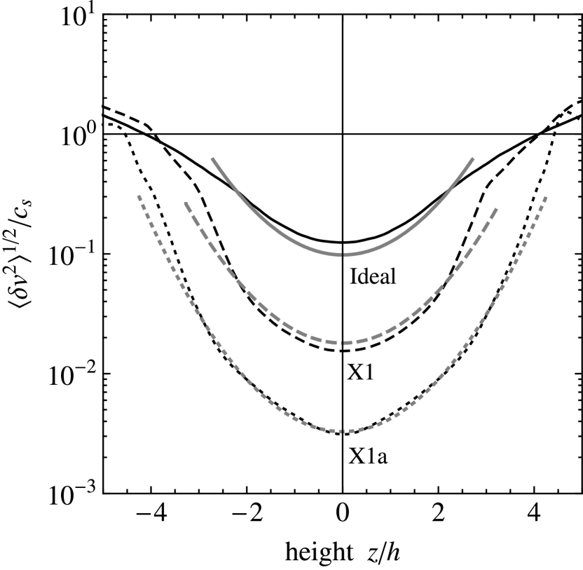
Figure 8.— Vertical profiles of the random velocity $\langle\delta v^{2}\rangle^{1/2}$ directly obtained from MHD simulations (black curves), compared with the predictions from Equation (22) with $\alpha_{\rm core}$ taken from Table 2 (gray curves). The solid, dashed, and dotted curves correspond to runs Ideal, X1, and X1a, respectively. The predicted profiles are plotted only at $|z|<h_{\rm ideal}$, where Equation (22) is valid.

5.1.2 Density Fluctuation

Density fluctuations generated by MRI-driven turbulence gravitationally interact with planetesimals and larger solid bodies, affecting their collisional and orbital evolution in protoplanetary disks (Laughlin et al., 2004; Nelson & Papaloizou, 2004; Nelson & Gressel, 2010; Gressel et al., 2011). Here, we examine how the amplitude of the density fluctuations is determined the vertically integrated accretion stress.

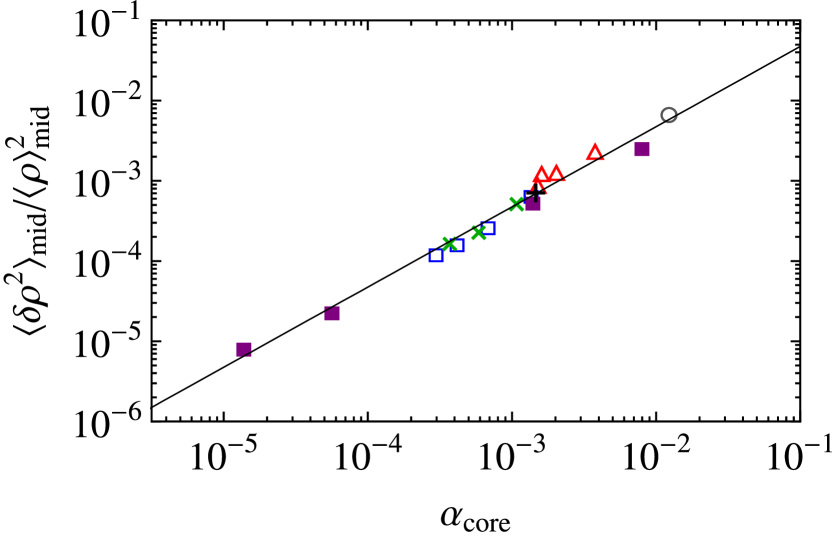
Figure 9.— Gas density fluctuation at the midplane, $\langle\delta\rho^{2}\rangle_{\rm mid}/\langle\rho\rangle_{\rm mid}^{2}$, versus $\alpha_{\rm core}$ for all runs presented in this study. The symbols correspond to models Ideal (circle), X0–X3 (open squares), Y1–Y4 (triangles), W1–Y3 (crosses), X1a–X1d (filled squares), and FS03L (plus sign). The line shows the best linear fit (Equation (23)).

As in Section 5.1.1, we begin with the analysis of the density fluctuations at the midplane, $\langle\delta\rho^{2}\rangle^{1/2}_{\rm mid}$. We find from Table 2 that $\langle\delta\rho^{2}\rangle_{\rm mid}$ more tightly correlates with $\alpha_{\rm core}$ than with $\alpha$. Figure 9 shows $\langle\delta\rho^{2}\rangle_{\rm mid}/\langle\rho\rangle_{\rm mid}$ versus $\alpha_{\rm core}$ for all runs. The best linear fit is given by

$$\langle\delta\rho^{2}\rangle_{\rm mid}=0.47\alpha_{\rm core}\langle\rho\rangle_{\rm mid}^{2},$$ (23)

which is shown by the solid line in Figure 9. If we use this equation with Equation (21), we can also obtain the relation between the velocity dispersion and density fluctuation, $\langle\delta v^{2}\rangle_{\rm mid}/c_{s}^{2}=1.7\langle\delta\rho^{2}\rangle_{\rm mid}/\langle\rho\rangle^{2}_{\rm mid}$. This is consistent with the idea that the fluctuations near the midplane are created by sound waves, for which $\delta v/c_{s}\sim\delta\rho/\rho$ (see also Section 4.1).

As shown in Section 4.1, $\langle\delta\rho^{2}\rangle$ is roughly proportional to $\langle\rho\rangle$ along the vertical direction in the disk core. Hence, if $\langle\delta\rho^{2}\rangle^{1/2}_{\rm mid}$ is given, one can reconstruct the vertical profile of the density fluctuation in the disk core according to

$$\langle\delta\rho^{2}\rangle \approx \langle\delta\rho^{2}\rangle_{\rm mid}\frac{\langle\rho\rangle}{\langle\rho\rangle_{\rm mid}}\approx\langle\delta\rho^{2}\rangle_{\rm mid}\exp\left(-\frac{z^{2}}{2h^{2}}\right)$$ (24)

$$\approx 0.47\alpha_{\rm core}\langle\rho\rangle_{\rm mid}^{2}\exp\left(-\frac{z^{2}}{2h^{2}}\right),$$

where we have used $\langle\rho\rangle\approx\langle\rho\rangle_{\rm mid}\exp(-z^{2}/2h^{2})$ and Equation (23) in the second and third equalities, respectively.

5.1.3 Outflow Flux

We have seen in Section 4.1 and Figure 4(f) that MRI drives outgoing gas flow at the outer boundaries of the active layers. The MRI-driven outflow has been first observed by Suzuki & Inutsuka (2009) in shearing-box simulations and been recently demonstrated by Flock et al. (2011) in global simulations. Suzuki & Inutsuka (2009) and Suzuki et al. (2010) point out that this outflow might contribute to the dispersal of protoplanetary disks, although it is still unclear whether the outflow can really escape from the disks (see below). Meanwhile, MRI also contributes to the accretion of the gas in the radial direction. For consistent modeling of these two effects, we seek how the accretion stress and outflow flux are correlated with each other.

We evaluate the outflow mass flux in the following way. As seen in Section 4.1, the temporally and horizontally averaged vertical mass flux $\langle\rho v_{z}\rangle$ is nearly constant at heights $|z|\gtrsim 5h$. Using this fact, we define the outflow mass flux $\dot{m}_{w}$ as the sum of $|\langle\rho v_{z}\rangle|$ averaged near upper and lower boundaries,

$$\dot{m}_{w}=\frac{\int_{h_{\rm bnd}-h}^{h_{\rm bnd}}|\langle\rho v_{z}\rangle|dz}{h}+\frac{\int_{-h_{\rm bnd}}^{-h_{\rm bnd}+h}|\langle\rho v_{z}\rangle|dz}{h},$$ (25)

where $h_{\rm bnd}=5\sqrt{2}h\approx 7h$ is the height of the upper and lower boundaries of the simulation box.

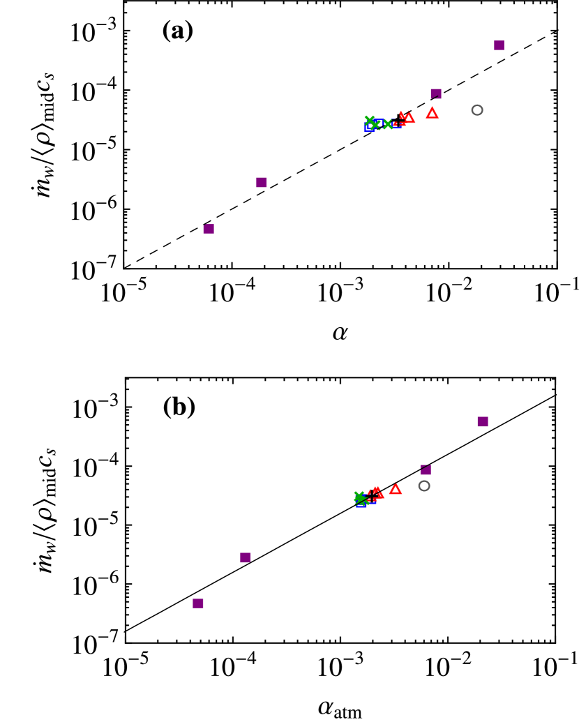
Figure 10.— Outflow mass flux $\dot{m}_{w}$ normalized by $\langle\rho\rangle_{\rm mid}c_{s}$ for all runs presented in this study. Panels (a) and (b) plot the data versus $\alpha$ and $\alpha_{\rm atm}$, respectively. The symbols correspond to models Ideal (circle), X0–X3 (open squares), Y1–Y4 (triangles), W1–W3 (crosses), X1a–X1d (filled squares), and FS03L (plus sign). The lines show the best linear fits (Equation (26) for panel (b)).

Figure 10(a) shows $\dot{m}_{w}$ normalized by $\langle\rho\rangle_{\rm mid}c_{s}$ versus $\alpha$ for all simulations. The dimensionless quantity $\dot{m}_{w}/(\langle\rho\rangle_{\rm mid}c_{s})$ is equivalent to $C_{w}$ used in Suzuki et al. (2010). For model Ideal, the value $\dot{m}_{w}=5\times 10^{-5}\langle\rho\rangle_{\rm mid}c_{s}$ is consistent with the $\beta_{z0}=10^{5}$ ideal run of Suzuki & Inutsuka (2009). The dashed line shows the best linear fit $\dot{m}_{w}/(\langle\rho\rangle_{\rm mid}c_{s})=0.015\alpha$. It can be seen that the linear fit captures a rough trend but still considerably overestimates the outflow flux for models Ideal and Y4. As seen in Table 2, these are the models in which $\alpha_{\rm core}$ dominates over $\alpha_{\rm atm}$. This implies that the turbulence in the disk core (which is the source of $\alpha_{\rm core}$) does not contribute to the outflow. In Figure 10(b), we replot the data by replacing $\alpha$ with $\alpha_{\rm atm}$. We find that $\dot{m}_{w}$ more tightly correlates with $\alpha_{\rm atm}$ than with $\alpha$. The best linear fit is found to be

$$\dot{m}_{w}=0.016\alpha_{\rm atm}\langle\rho\rangle_{\rm mid}c_{s}.$$ (26)

This result is consistent with the idea that the outflow is driven at the outer boundaries of the active layers (Suzuki & Inutsuka, 2009), because the dominant contribution to $\alpha_{\rm atm}$ comes from heights very close to $h_{\rm ideal}$.

Although outflow from the simulation box is a general phenomenon in our simulations, it is unclear whether the outflow leaves or returns to the disk. In fact, the outflow velocity observed in our simulations does not exceed the sound speed even at the vertical boundaries. Since the escape velocity is higher than the sound speed, this means that the outflow does not have an outward velocity enough to escape out of the disk. Acceleration of the outflow beyond the escape velocity has not been directly demonstrated by previous simulations as well (Suzuki et al., 2010; Flock et al., 2011). However, Suzuki et al. (2010) point out a possibility that magnetocentrifugal forces and/or stellar winds could accelerate the outflow to the escape velocity. If the escape of the outflow will be confirmed in the future, our scaling formula for $\dot{m}_{w}$ will certainly become a useful tool to discuss the dispersal of protoplanetary disks.

5.2. Saturation Predictors for the Accretion Stresses

In the previous subsection, we have shown that the amplitudes of various turbulent quantities scale with the vertically integrated stresses $\alpha_{\rm core}$ and $\alpha_{\rm atm}$. The next step is to find out how to predict $\alpha_{\rm core}$ and $\alpha_{\rm atm}$ in the saturated state from the vertical magnetic flux $B_{z0}$ (or equivalently $\beta_{z0}$) and the resistivity profile $\eta$. As shown in Section 4.2, the turbulent state of a disk depends on the resistivity only through the critical heights of the dead zone, $h_{\Lambda}$ and $h_{\rm res}$. Furthermore, the values of $h_{\Lambda}$ and $h_{\rm res}$ are only weakly affected by the nonlinear evolution of MRI since the fluctuations in $B_{z}$ and $\rho$ are small inside the dead zone (see Section 4.1). Therefore, we expect that the effect of the resistivity can be well predicted by the values of $h_{\Lambda}$ and $h_{\rm res}$ in the initial state, i.e., $h_{\Lambda,0}$ and $h_{{\rm res},0}$. With this expectation, we try to derive saturation predictors for $\alpha_{\rm core}$ and $\alpha_{\rm atm}$ as a function of $\beta_{z0}$, $h_{\Lambda,0}$, and $h_{{\rm res},0}$.

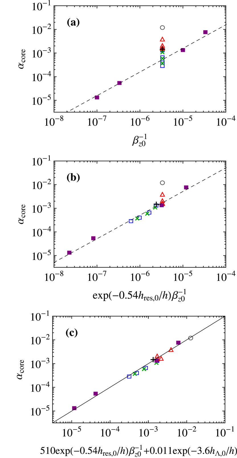
Figure 11.— Disk core accretion stress $\alpha_{\rm core}$ for all our simulations. (a) Vs. the inverse initial plasma beta $\beta_{z0}^{-1}$. (b) Vs. $\beta_{z0}^{-1}$ multiplied by $\exp(-0.54h_{{\rm res},0}/h)$ (see also Figure 12). (c) Vs. the final predictor function, Equation (28) (solid line). The symbols correspond to models Ideal (circle), X0–X3 (open squares), Y1–Y4 (triangles), W1–Y3 (crosses), X1a–X1d (filled squares), and FS03L (plus sign). The dashed lines in panels (a) and (b) are linear fits, shown only for reference.

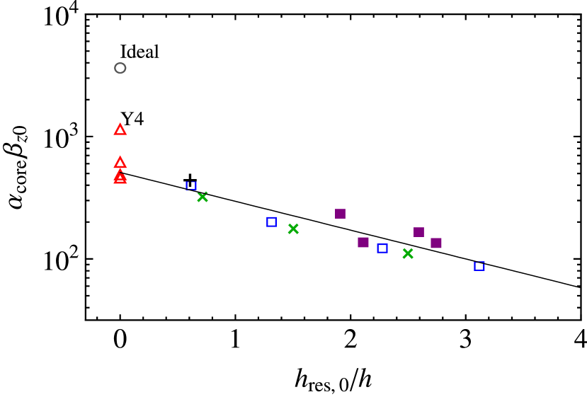
Figure 12.— $\alpha_{\rm core}\beta_{z0}$ versus $h_{{\rm res},0}$ for all runs. The symbols correspond to models Ideal (circle), X0–X3 (open squares), Y1–Y4 (triangles), W1–W3 (crosses), X1a–X1d (filled squares), and FS03L (plus sign). The solid line shows an exponential fit for runs except Ideal and Y4 (Equation (27)).

First, we focus on $\alpha_{\rm core}$. Figure 11(a) plots $\alpha_{\rm core}$ versus $\beta^{-1}_{z0}$ for all our simulations. We see that $\alpha_{\rm core}$ scales roughly linearly with $\beta^{-1}_{z0}$. The deviation from the linear scaling is expected to come from the difference in the dead zone size, i.e., $h_{\Lambda,0}$ and $h_{{\rm res},0}$. In Figure 12, we plot the product $\alpha_{\rm core}\beta_{z0}$ as a function of $h_{{\rm res},0}$. For models except Ideal and Y4, we find that $\alpha_{\rm core}\beta_{z0}$ is well predicted by a simple formula

$$\alpha_{\rm core}\beta_{z0}=510\exp(-0.54h_{{\rm res},0}/h).$$ (27)

Figure 11(b) replot the data in Figure 11(a) by replacing $\beta^{-1}_{z0}$ with $\exp(-0.54h_{{\rm res},0}/h)\beta^{-1}_{z0}$. For models Ideal and Y4, Equation (27) underestimates $\alpha_{\rm core}$. As explained in Section 4.2, these models exhibit higher magnetic activity near the midplane than the other models because of no or a thin dead zone $(2h_{\Lambda}<h)$. We expect that the higher magnetic activity gives additional contribution to $\alpha_{\rm core}$. Taking into account this effect, we arrive at the final predictor function,

$$\alpha_{\rm core}=510\exp(-0.54h_{{\rm res},0}/h)\beta^{-1}_{z0}+0.011\exp(-3.6h_{\Lambda,0}/h).$$ (28)

Here, the numerical factors $0.011$ and $3.6$ appearing in the second term have been chosen to reproduce the results of runs Ideal and Y4, respectively. Figure 11(c) compares the final fitting formula with the numerical data. It can be seen that Equation (28) well predicts $\alpha_{\rm core}$ for all our models. Note that the second term of the predictor function is assumed to have no explicit linear dependence on $\beta_{z0}^{-1}$ unlike the first term. In fact, it is possible to reproduce our data by multiplying the second term by a prefactor $3\times 10^{5}/\beta_{z0}$. However, as we will see below, the absence of the prefactor makes the predictor function consistent with the results of ideal MHD simulations in the literature.

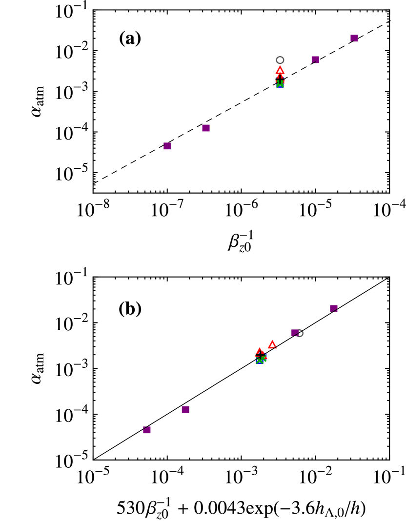
Figure 13.— Atmosphere accretion stress $\alpha_{\rm atm}$ for all our simulations. (a) Vs. the inverse initial plasma beta $\beta_{z0}^{-1}$. (b) Vs. the final predictor function, Equation (29) (solid line). The symbols correspond to models Ideal (circle), X0–X3 (open squares), Y1–Y4 (triangles), W1–W3 (crosses), X1a–X1d (filled squares), and FS03L (plus sign). The dashed line in panel (a) is a linear fit, only shown for reference.

The predictor function for $\alpha_{\rm atm}$ can be obtained in a similar way. Figure 13(a) shows $\alpha_{\rm atm}$ versus $\beta_{z0}^{-1}$ for all our runs. We find that a simple linear relation $\alpha_{\rm atm}=530\beta_{z0}^{-1}$ well fits to the data except for models Ideal and Y4. This means that $\alpha_{\rm atm}$ is characterized only by $\beta_{z0}^{-1}$ as long as the dead zone is thick $(2h_{\Lambda}>h)$. To take into account the cases of thin dead zones, we add a term proportional to $\exp(-3.6h_{\Lambda,0}/h)$ as has been done for $\alpha_{\rm core}$, and obtain

$$\alpha_{\rm atm}=530\beta^{-1}_{z0}+0.0043\exp(-3.6h_{\Lambda,0}/h),$$ (29)

where the prefactor $0.0043$ for the second term has been determined to fit to the result of run Ideal. As seen in Figure 13(b), Equation (29) well predicts the value of $\alpha_{\rm atm}$ for all our runs.

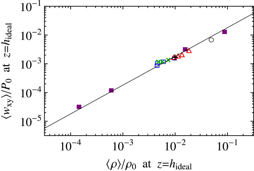
Figure 14.— Accretion stress $\langle w_{xy}\rangle$ versus gas density $\langle\rho\rangle$ at the upper boundary of the active layer ($z=h_{\rm ideal}$) for all runs. The symbols correspond to models Ideal (circle), X0–X3 (open squares), Y1–Y4 (triangles), W1–Y3 (crosses), X1a–X1d (filled squares), and FS03L (plus sign). The solid line shows a linear fit (Equation (30)).

Our predictor functions indicate that the vertically integrated accretion stress is inversely proportional to $\beta_{z0}$ when a large dead zone is present ($h_{\Lambda}\gtrsim h$). As we show below, this dependence originates from the magnitude of the accretion stress at the outer boundaries of the active layers, $|z|\approx h_{\rm ideal}$. When a dead zone exists, the dominant contribution to $\alpha$ comes from the accretion stress at that location (see Figures 5 and 6). As shown Figure 14, our simulations suggest that the accretion stress at $|z|=h_{\rm ideal}$ obeys a simple relation

$$\langle w_{xy}\rangle(h_{\rm ideal})\approx 0.18\langle\rho\rangle(h_{\rm ideal})c_{s}^{2}.$$ (30)

This means that the averaged accretion stress at $|z|=h_{\rm ideal}$ is $18\%$ of the averaged gas pressure $\langle\rho c_{s}^{2}\rangle$ at the same height. By the definition of $h_{\rm ideal}$, the gas density at $|z|=h_{\rm ideal}$ is related to $\langle B_{z}^{2}\rangle$ at the same height as $\langle\rho\rangle(h_{\rm ideal})=(2\pi)^{2}\langle B_{z}^{2}\rangle(h_{\rm ideal})/4\pi c_{s}^{2}$. Since our simulations suggest $\langle B_{z}^{2}\rangle(h_{\rm ideal})\sim 10B_{z0}^{2}$, the relation means $\langle\rho\rangle(h_{\rm ideal})\sim 10(2\pi)^{2}B_{z0}^{2}/4\pi c_{s}^{2}\sim 10^{3}\beta_{z0}^{-1}\rho_{0}$. Using this fact, Equation (30) can be rewritten into the linear relation between $\langle w_{xy}\rangle(h_{\rm ideal})$ and $\beta_{z0}^{-1}$:

$$\langle w_{xy}\rangle(h_{\rm ideal})\sim 100\beta_{z0}^{-1}\rho_{0}c_{s}^{2}.$$ (31)

When a dead zone is present, the level of $\alpha$ is determined by $\langle w_{xy}\rangle(h_{\rm ideal})$ (see above), so we have $\alpha\propto\beta_{z0}^{-1}$.

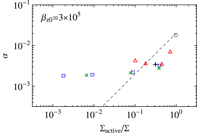
Figure 15.— Vertically integrated accretion stress $\alpha$ versus the column density $\Sigma_{\rm active}$ of the active layer for $\beta_{z0}=3\times 10^{5}$ models. The symbols correspond to models Ideal (circle), X0–X3 (open squares), Y1–Y4 (triangles), W1–Y3 (crosses), and FS03L (plus sign). The dashed line is a linear function, only shown for reference.

We remark that the vertically integrated stress does not scale linearly with the column density of active layers. This is shown in Figure 15, where we compare $\alpha$ with the column density $\Sigma_{\rm active}$ of the active region $h_{\Lambda}<|z|<h_{\rm ideal}$. We see that $\alpha$ decreases much more slowly than $\Sigma_{\rm active}$ when $\Sigma_{\rm active}$ is less than $10\%$ of the total gas surface density. This reflects the fact that the dominant contribution to $\alpha$ comes from the outer boundaries of the active zones, $|z|\approx h_{\rm ideal}$.

It is useful to see how the predictor functions work when a dead zone is absent. If $h_{\Lambda,0}=h_{{\rm res},0}=0$, Equations (28) and (29) predict the total accretion stress $\alpha=1.0\times 10^{3}\beta_{z0}^{-1}+0.015$. This implies that $\alpha$ is constant ($\alpha\approx 10^{-2}$) for $\beta_{z0}\gtrsim 10^{5}$ and increases linearly with $\beta_{z0}^{-1}$ ($\alpha\approx 10^{-2}(10^{5}/\beta_{z0})$) for $\beta_{z0}\lesssim 10^{5}$. Strikingly, this prediction is consistent with the finding by Suzuki et al. (2010, see their Figure 2). The existence of the floor value $\alpha\approx 10^{-2}$ at low net vertical magnetic fluxes (i.e., at high $\beta_{z0}$) is also supported by recent stratified MHD simulations with zero net flux (Davis et al., 2010). These facts suggest that our predictor functions are applicable even when a dead zone is absent.

6. Vertical Diffusion Coefficient

As seen in Section 4, sound waves excited in the upper layers create fluctuations in the gas velocity near the midplane. It has been well known that fully developed MRI-driven turbulence causes the diffusion of small dust particles (Johansen & Klahr, 2005; Turner et al., 2010). However, it has not been fully understood how the sound waves propagating inside a dead zone affect the dynamics of dust particles there. For example, Suzuki & Inutsuka (2009) speculated that the sound waves might promote dust sedimentation by transferring the downward momentum to dust particles. On the other hand, Turner et al. (2010) reported that the waves excite vertical oscillation of dust particles deep inside the dead zone and thus prevent the formation of a thin dust layer. Since dust sedimentation is crucial to planetesimal formation via gravitational instability, it is worth addressing here how it is affected by the velocity dispersion created by sound waves.

Figure 16.— Temporal evolution of the dust density at the midplane in various MHD runs. The four panels show the results for models Ideal (upper left), X1 (upper right), X3 (lower left), and Y1 (lower right). The solid curves show the horizontally averaged dust density $\rho_{d,{\rm mid}}$ observed in the MHD runs, while the dotted curve show the evolution of $\rho_{d,{\rm mid}}$ in a laminar disk. The dashed curves are the predictions from the one-dimensional advection-diffusion equation (Equation (33)). The diffusion coefficient $D_{z}$ in Equation (33) is assumed to be proportional to $\langle\delta v_{z}^{2}\rangle/\Omega$, and the proportionality factor has been chosen to best reproduce the evolution of $\rho_{d,{\rm mid}}$ in the MHD runs.

Here, we focus on the dynamics of small dust particles, and model the swarm of the particles as a passive scalar as was previously done by Johansen & Klahr (2005) and Turner et al. (2010). We assume that dust particles are so small and their stopping time $\tau_{s}$ is much shorter than the turnover time of turbulence ($\sim\Omega^{-1}$). We also assume that the dust density is lower than the gas density and hence the dust has no effect on the gas motion. Under these assumptions, the velocity of dust particles relative to the gas can be approximated by the terminal velocity ${\bf V}_{T}=-\Omega^{2}\tau_{s}z\hat{{\bf z}}$, where $\hat{{\bf z}}$ is the unit vector for the $z$–direction. Then, the equation of continuity for dust is given by

$$\frac{\partial\rho_{d}}{\partial t}+\nabla\cdot[\rho_{d}({\bf v}+{\bf V}_{T})]=0,$$ (32)

where $\rho_{d}$ is the dust density. Equation (32) has an advantage that the time step can be taken longer than $\tau_{s}$ in numerical calculation.

We have solved Equation (32) for four models (Ideal, X1, X3, and Y1) with the initial condition that the dust-to-gas mass ratio $f\equiv\rho_{d}/\rho$ is constant throughout the simulation box. To extract the effect of the quasi-stationary turbulence, we insert the dust 100 (for models X1, X3, and Y1) or 250 (for model Ideal) orbits after the beginning of the MHD calculations. The stopping time $\tau_{s}$ is set to $\tau_{s}=0.01\Omega^{-1}$ for model Ideal and $\tau_{s}=0.001\Omega^{-1}$ for the other models. The longer $\tau_{s}$ has been adopted for model Ideal to allow the dust to settle appreciably in the stronger turbulence. In reality, the stopping time of a dust particle depends on the gas density and hence on $z$, but we ignore this dependency for simplicity.

Figure 16 shows the temporal evolution of the dust density at the midplane, $\rho_{d,{\rm mid}}$, for the four MHD runs. The solid curves show the horizontally averaged $\rho_{d,{\rm mid}}$ observed in the MHD runs. For comparison, the evolution of $\rho_{d,{\rm mid}}$ in a hydrostatic, laminar disk is also shown by the dotted curves. Irrespectively of the presence or absence of a dead zone, the dust density observed in the MHD runs is higher than that in a laminar disk at all moments. This means that sound waves propagating in a dead zone do not promote but prevent dust settling as turbulence does in an active zone.

To illustrate more clearly the diffusive nature of the velocity dispersion in a dead zone, we try to compare the above results with a simple advection-diffusion theory. Here, we consider a one-dimensional advection-diffusion equation (Dubrulle et al., 1995)

$$\frac{\partial\rho_{d}}{\partial t}=-\frac{\partial(\rho_{d}V_{T})}{\partial z}+\frac{\partial}{\partial z}\left(D_{z}\rho\frac{\partial}{\partial z}\frac{\rho_{d}}{\rho}\right),$$ (33)

where $V_{T}$ is the terminal velocity given above and $D_{z}$ is the vertical diffusion coefficient for dust. If the dust particles are sufficiently small ($\tau_{s}\Omega\ll 1$), $D_{z}$ is equal to the diffusion coefficient for gaseous contaminants (e.g., Youdin & Lithwick, 2007). The first term in the right-hand side of Equation (33) represents the downward advection of dust due to settling, while the second term represents the diffusion of dust in the stratified gas. For disks with no or a small ($|z|\lesssim h$) dead zone, it is known that Equation (33) well describes the evolution of $\rho_{d}$ if the diffusion coefficient is assumed to be (Fromang & Papaloizou, 2006)

$$D_{z}\approx\langle\delta v_{z}^{2}\rangle/\Omega.$$ (34)

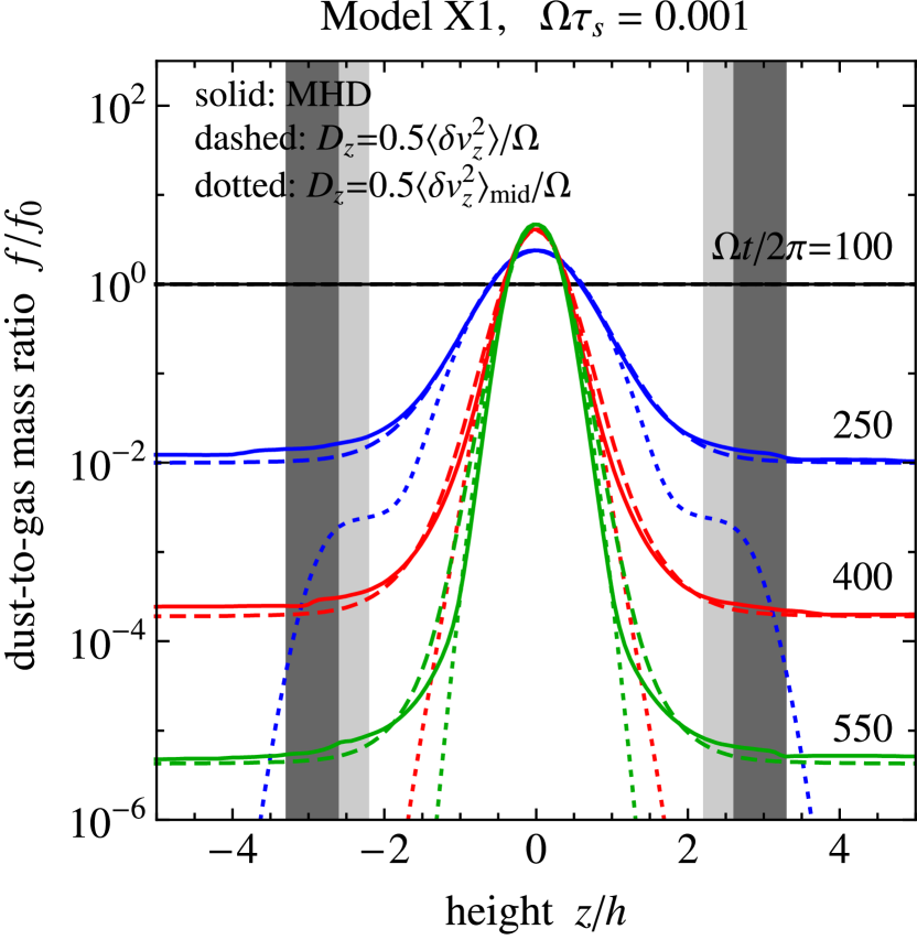
Figure 17.— Snapshots of the vertical distribution of the dust-to-gas mass ratio $f=\rho_{d}/\rho$ at $t=100$, 250, 400, and 550 orbits for model X1. The solid curves show the horizontally averaged $f$ observed in the MHD simulation. The dashed curves show the solutions to the one-dimensional advection-diffusion equation (Equation (33)) with $D_{z}(z)=0.5\langle\delta v_{z}^{2}\rangle(z)/\Omega$. The dotted curves show the solution to Equation (33) with a constant diffusion coefficient $D_{z}=0.5\langle\delta v_{z}^{2}\rangle_{\rm mid}/\Omega$.

We here examine whether Equations (33) and (34) work well even when a dead zone is present. We solve Equation (33) with $D_{z}=b\langle\delta v_{z}^{2}\rangle/\Omega$, where the vertical distribution of $\langle\delta v_{z}^{2}\rangle$ is taken from temporally and horizontally averaged MHD data and $b$ is a dimensionless fitting parameter. The dashed curves in Figure 16 show the predictions by the advection-diffusion model, where $b$ is set to be $1.0$, $0.5$, $0.9$, and $1.0$ for runs Ideal, X1, X3, and Y1, respectively. It can be seen that the advection-diffusion model with $b\sim 1$ successfully reproduces the long-term evolution of the observed $\rho_{d,{\rm mid}}$ for all the models. It is striking that a constant $b$ well reproduces the evolution of the dust density at all heights, as is shown in Figure 17. In this figure, the solid and dashed curves show the vertical distribution of the dust-to-gas mass ratio $f=\rho_{d}/\rho_{g}$ observed in run X1 and predicted by the advection-diffusion model with $b=0.5$, respectively. In this run, the boundaries between the active and dead zones are located at $|z|=h_{\Lambda}\approx 2.5h$ (see Table 2). However, Equation (33) successfully predicts the evolution of $f$ even if we do not change the value of $b$ across the boundaries. This fact supports the idea that sound waves propagating across a dead zone contribute to the diffusion of dust particles just as turbulence does in active zones.

It is worth mentioning here that the diffusion coefficient $D_{z}$ increases with $|z|$ as has been pointed out by Turner et al. (2006) and Fromang & Nelson (2009). This effect is particularly significant at high altitudes where the gas density is much lower than that at the midplane, because $D_{z}\propto\langle\delta v^{2}_{z}\rangle$ is roughly proportional to the inverse of the gas density. The dotted curves in Figure (17) show how Equation (33) would fail to predict dust evolution if one assumed a constant diffusion coefficient $D_{z}=0.5\langle\delta v^{2}_{z}\rangle_{\rm mid}/\Omega$. We see that the constant diffusion coefficient model significantly underestimates the dust density at $|z|\gg h$. This fact will merit consideration when modeling the chemical evolution of protoplanetary disks, in which the vertical mixing of molecules is of importance (Heinzeller et al., 2011).

Finally, we give a simple analytic recipe for the vertical distribution of $D_{z}$. It is useful to rewrite Equation (34) in terms of $\langle\delta v^{2}\rangle$, for which the scaling relation (Equation (22)) and predictor function (Equation (28)) are available. Table 2 lists the ratio of $\langle\delta v_{z}^{2}\rangle_{\rm mid}$ to $\langle\delta v^{2}\rangle_{\rm mid}$ for all our simulations. It can be seen that $\langle\delta v_{z}^{2}\rangle_{\rm mid}\approx(32\%\pm 15\%)\times\langle\delta v^{2}\rangle_{\rm mid}$, indicating that $\langle\delta v_{z}^{2}\rangle_{\rm mid}$ is roughly equal to a third of $\langle\delta v^{2}\rangle_{\rm mid}$. Furthermore, the ratio $\langle\delta v_{z}^{2}\rangle/\langle\delta v^{2}\rangle$ is approximately constant in the disk core, as is illustrated in Figure 4(c). Based on these facts, we approximate $\langle\delta v_{z}^{2}\rangle$ as $\langle\delta v^{2}\rangle/3$ in the disk core. Using this approximation together with the scaling relation for $\langle\delta v^{2}\rangle$ (Equation (22)), we rewrite Equation (34) as

$$D_{z} \approx \frac{1}{3}\langle\delta v^{2}\rangle/\Omega$$ (35)

$$\approx 0.3(\alpha_{\rm core}c_{s}^{2}/\Omega)\exp\biggl{(}{\displaystyle\frac{z^{2}}{2h^{2}}}\biggr{)}.$$

If one uses this equation together with the predictor function for $\alpha_{\rm core}$ (Equation (28)), one can calculate the vertical distribution of $D_{z}$ in the disk core for given $\beta_{z0}$ and $\eta$.

7. Discussion: Effects of Numerical Resolution

All MHD simulations presented in the previous sections were performed with the numerical resolution of $40\times 80\times 200$ grid cells for the simulation box of size $2\sqrt{2}h\times 8\sqrt{2}h\times 10\sqrt{2}h$. Here, we examine how the numerical resolution affects the saturated state of turbulence.

Figure 18.— Saturated values of various quantities versus numerical resolution for model X1. From top to bottom: $\alpha$, $\alpha_{\rm core}$, $\langle\delta v^{2}\rangle_{\rm mid}/c_{s}^{2}$, $\langle\delta\rho^{2}\rangle_{\rm mid}/\langle\rho\rangle_{\rm mid}^{2}$, and $\dot{m}_{w}/\langle\rho\rangle_{\rm mid}c_{s}$. The horizontal axis shows the number of grid cells per length $\sqrt{2}h$ in the vertical direction, $n_{z}$. The value $n_{z}=20$ corresponds to the resolution adopted in this study.

We carry out X1 simulations with changing the numerical resolution to $20\times 40\times 100$ cells and $80\times 160\times 400$ cells. Figure 18 compares the saturated values of various quantities obtained from the two runs with the values from the original X1 run (Table 2). Here, the horizontal axis shows the number of grid cells per length $\sqrt{2}h$ in the vertical direction, $n_{z}$ (see footnote 1). The value $n_{z}=20$ corresponds to our original resolution. We see that the change of the resolution hardly affects the integrated accretion stresses $\alpha$ and $\alpha_{\rm core}$ and outflow flux $\dot{m}_{w}$, suggesting that the resolution of $n_{z}=20$ is sufficient for these quantities to converge well. By contrast, the velocity and density dispersions $\langle\delta v^{2}\rangle_{\rm mid}$ and $\langle\delta\rho^{2}\rangle_{\rm mid}$ increase with improving the resolution. Since the energy input rate to turbulence should be the same if the integrated accretion stress is unchanged, the resolution dependence of the velocity and density dispersions is expected to mainly come from artificial dissipation of sound waves in the simulation box. However, we also see that this effect becomes less significant as the resolution is improved. Detailed inspection shows that the fractional increase in $\langle\delta v^{2}\rangle_{\rm mid}$ is $81\%$ when going from $n_{z}=10$ to $n_{z}=20$ but is $40\%$ when going from $n_{z}=20$ to $n_{z}=40$. This suggests that the amplitudes of the velocity and density fluctuations should converge to finite values in the limit of high resolutions ($n_{z}\to\infty$). This is to be expected, since sound waves in a stratified disk physically dissipate through, e.g., shock formation, particularly at high altitudes where the gas density is low and therefore the amplitudes of the waves become large. We find that the data for $\langle\delta v^{2}\rangle_{\rm mid}/c_{s}^{2}$ shown in Figure 18 lie on a curve $\langle\delta v^{2}\rangle_{\rm mid}/c_{s}^{2}=0.012-0.0015n_{z}^{-0.15}$. This implies a converged value of $\langle\delta v^{2}\rangle_{\rm mid}/c_{s}^{2}\approx 0.012$, which is five times higher than that obtained in our $n_{z}=20$ simulation ($\langle\delta v^{2}\rangle_{\rm mid}/c_{s}^{2}\approx 0.0024$). From this estimate, we see that $\langle\delta v^{2}\rangle$ and $\langle\delta\rho^{2}\rangle$ could be underestimated by a factor of several in the simulations presented in this study.

In summary, we find that the outflow mass flux and vertically integrated accretion stress converge well within our numerical resolution. This suggests that the predictor functions for $\alpha_{\rm core}$ and $\alpha_{\rm atm}$ (Equations (28) and (29)) and the scaling relation between $\dot{m}_{w}$ and $\alpha_{\rm atm}$ are hardly affected by the resolution. On the other hand, the amplitudes of sound waves could be underestimated by a factor of several because of the finite grid size. Future high-resolution simulations will enable to better quantify the scaling relations between $\langle\delta v^{2}\rangle$ and $\alpha_{\rm core}$ and between $\langle\delta\rho^{2}\rangle$ and $\alpha_{\rm core}$ (Equations (22) and (24)).

8. Summary

Good knowledge about the turbulent structure of protoplanetary disks is essential for understanding planet formation. To provide an empirical basis for modeling the coevolution of dust and MRI, we have performed MHD simulations of a vertically stratified shearing box with an MRI-inactive “dead zone” of various sizes and with a vertical magnetic flux of various strengths. Our findings are summarized as follows.

1. We have introduced the critical heights ($h_{\rm ideal}$, $h_{\Lambda}$, and $h_{\rm res}$) that characterize the MRI in a stratified disk (Section 3). We have found that the vertical structure of MRI-driven turbulence depends on the resistivity profile only through the critical heights for the dead zone ($h_{\Lambda}$ and $h_{\rm res}$) and is insensitive to the detail of the resistivity profile (Section 4.2).

2. In the “disk core” ($|z|<h_{\rm ideal}$), the density-weighted velocity dispersion $\langle\rho\rangle\langle\delta v^{2}\rangle$ is nearly constant along the vertical direction (Section 4.1). This means that the velocity dispersion is approximately inversely proportional to the gas density. Weak dependence on $z$ is also found for $\langle\delta\rho^{2}\rangle/\langle\rho\rangle$, meaning that the density fluctuation $\langle\delta\rho^{2}\rangle^{1/2}$ is proportional to the square root of the averaged density.

3. The accretion stresses in the disk core and “atmosphere” ($|z|>h_{\rm ideal}$) differently contribute to the turbulent structure of a disk (Section 5.1). The velocity dispersion $\langle\delta v^{2}\rangle$ and density fluctuation $\langle\delta\rho^{2}\rangle$ in the disk core depend linearly on the accretion stress integrated over the core, $\alpha_{\rm core}$ (Equations (21) and (23)). By contrast, the outflow mass flux $\dot{m}_{w}$ depends linearly on the stress integrated over the atmosphere, $\alpha_{\rm atm}$ (Equation (26)).

4. We have obtained simple empirical formulae that predict the vertically integrated stresses $\alpha_{\rm core}$ and $\alpha_{\rm atm}$ in the saturated state (Section 5.2; Equations (28) and (29)). These are written as a function of the strength of the vertical magnetic flux (or $\beta_{z0}$) and the critical heights of the dead zone measured in the nonturbulent state ($h_{{\rm res},0}$ and $h_{\Lambda,0}$). These predictor functions together with the saturation relations described above allow to calculate various turbulent quantities for a given resistivity profile and a net vertical flux.

5. We have confirmed that the vertical diffusion coefficient $D_{z}$ of contaminants is given by $D_{z}\approx\langle\delta v_{z}^{2}\rangle/\Omega$ both inside and outside a dead zone (Section 6). This implies that sound waves propagating across a dead zone contribute to the diffusion of dust particles just as turbulence does in active zones. We have obtained a simple analytic recipe for the vertical distribution of $D_{z}$ as a function of $\alpha_{\rm core}$ on the basis of our MHD simulation data (Equation (35)).

The empirical formulae obtained in this study enable us to predict the amplitudes of various turbulent quantities in a protoplanetary disk with a dead zone. The steps to be performed are as follows.

1. Prepare the vertical profile of the ohmic resistivity $\eta$, and find $h_{\Lambda}$ and $h_{\rm res}$ from Equations (12) and (13). A realistic profile of $\eta$ in the presence of dust particles can be obtained by solving the ionization state of the gas and the charge state of the dust simultaneously (e.g., Sano et al., 2000; Ilgner & Nelson, 2006; Okuzumi, 2009).

2. Calculate $\alpha_{\rm core}$ and $\alpha_{\rm atm}$ using the predictor functions, Equations (28) and (29).

3. One can now calculate the turbulent viscosity of the disk as $\nu_{\rm turb}=(3/2)(\alpha_{\rm core}+\alpha_{\rm atm})c_{s}^{2}/\Omega$ (see Equations (18), (19), and (20)). The vertical distribution of the gas velocity dispersion and density fluctuation in the disk core ($|z|<h_{\rm ideal}$) can be calculated from Equations (22) and (24), respectively. The outflow mass flux can be evaluated from Equation (26). For the diffusion coefficient in the disk core, one can use Equation (35).

When using our empirical formulae, it should be kept in mind that our scaling relations for velocity and density fluctuations (Equation (22) and (24)) could underestimate their mean-squared amplitudes relative to the integrated accretion stress by a factor of several because of the numerical dissipation of sound waves (Section 7). Future high-resolution simulations will allow to better quantify the saturation level of sound wave amplitudes.

Appendix A Ionization Degree and Ohmic Resistivity in Protoplanetary Disks

In this Appendix, we explain how the resistivity profile adopted in this study (Equation (4)) is related to realistic resistivity profiles in protoplanetary disks. Since the resistivity is inversely proportional to the ionization degree (more precisely, the electron abundance; see Blaes & Balbus 1994), we will see how the ionization degree depends on the height $z$ above the midplane.

Recombination occurs in the gas phase and on dust surfaces. The gas-phase recombination dominates if the total surface area of dust particles is negligibly small. In this case, the equation for the ionization-recombination equilibrium is given by

$$\zeta n_{n}=\gamma_{ie}n_{i}n_{e}=\gamma_{ie}n_{e}^{2},$$ (A1)

where $\zeta$ is the ionization rate (the probability per unit time at which a molecule is ionized), $n_{n}$, $n_{i}$ , and $n_{e}$ are the number densities of neutrals, ions, and electrons, respectively, and $\gamma_{ie}$ is the gas-phase recombination rate coefficient. The second equality in the above equation assumes the charge neutrality in the gas phase, $n_{i}=n_{e}$. Equation (A1) leads to the electron abundance

$$x_{e}=\frac{n_{e}}{n_{n}}=\sqrt{\frac{\zeta}{\gamma_{ie}n_{n}}}\propto\sqrt{\zeta}\exp\biggl{(}{\displaystyle\frac{z^{2}}{4h^{2}}}\biggr{)},$$ (A2)

which means that the resistivity is proportional to $\zeta^{-1/2}\exp(-z^{2}/4h^{2})$. Thus, if the vertical dependence of $\zeta$ can be neglected, the resistivity profile is given by Equation (4) with $h_{\eta}=\sqrt{2}h$. Note that Equation (5) is derived instead of Equation (4) if cosmic-ray ionization is assumed and the attenuation of cosmic rays toward the midplane is taken into account (Fleming & Stone, 2003).

If the total surface area of dust particles is large, recombination occurs mainly on dust surfaces. In this case, the equation for the ionization-recombination equilibrium is given by

$$\zeta n_{n}=\gamma_{de}n_{d}n_{e},$$ (A3)

where $\gamma_{de}$ is the sticking rate coefficient for dust–electron collision and $n_{d}$ is the number density of dust particles. The sticking rate coefficient depends on the charge of the dust particles, and ultimately on $n_{e}$ via the charge neutrality (see Okuzumi, 2009), but we will ignore this dependence in the following. From Equation (A3) , we have

$$x_{e}=\frac{\zeta}{\gamma_{de}n_{d}}\propto\zeta\exp\biggl{(}{\displaystyle\frac{z^{2}}{2h_{d}^{2}}}\biggr{)},$$ (A4)

where we have assumed that $n_{d}\propto\exp(-z^{2}/h_{d}^{2})$ with $h_{d}$ being the scale height of the dust particles (in fact, one can show using Equation (33) that $n_{d}$ obeys a Gaussian distribution in sedimentation-diffusion equilibrium if $D_{z}\propto\tau_{s}\propto n_{g}^{-1}\propto\exp(z^{2}/2h^{2})$; the condition $\tau_{s}\propto n_{g}^{-1}$ is satisfied if the size of the dust particles is smaller than the mean free path of the gas). Thus, ignoring the dependence of $\zeta$ on $z$, the resistivity $\eta\propto x_{e}^{-1}$ is given by Equation (4) with $h_{\eta}=h_{d}$.

References

- Bai & Stone (2010) Bai, X.-N., & Stone, J. 2010, ApJ, 722, 1437
- Balbus & Hawley (1991) Balbus, S. A., & Hawley, J. F. 1991, ApJ, 376, 214
- Balbus & Papaloizou (1999) Balbus, S. A., & Papaloizou, J. C. B. 1999, ApJ, 521, 650
- Blaes & Balbus (1994) Blaes, O. M., & Balbus, S. A. 1994, ApJ, 421, 163
- Brauer et al. (2008) Brauer, F., Dullemond, C. P., & Henning, Th. 2008, A&A, 480, 859
- Chambers & Wetherill (1998) Chambers, J. E., & Wetherill, G. W. 1998, Icarus, 136, 304
- Cuzzi et al. (2001) Cuzzi, J. N., Hogan, R. C., Paque, J. M., & Dobrovolskis, A. R. 2001, ApJ, 546, 496
- Cuzzi et al. (2008) Cuzzi, J. N., Hogan, R. C., & Shariff, K. 2008, ApJ, 687, 1432
- Cuzzi et al. (2010) Cuzzi, J. N., Hogan, R. C., Bottke, W. F. & 2010, Icarus, 208, 518
- Davis et al. (2010) Davis, S. W., Stone, J. M., Pessah, M. E. 2010, ApJ, 713, 52
- Dubrulle et al. (1995) Dubrulle, B., Morfill, G., & Sterzik, M. 1995, Icarus, 114, 237
- Dullemond & Dominik (2005) Dullemond, C. P., & Dominik, C. 2005, A&A, 434, 971
- Flaig et al. (2010) Flaig, M., Kley, W., & Kissmann, R., MNRAS, 409, 1297
- Fleming & Stone (2003) Fleming, T., & Stone, J. M. 2003, ApJ, 585, 908
- Flock et al. (2011) Flock, M., Dzyurkevich, N., Klahr, H., Turner, N. J., & Henning, Th. 2011, ApJ, 735, 122
- Fromang & Nelson (2009) Fromang, S., & Nelson, R. P. 2009, A&A, 496, 597
- Fromang & Papaloizou (2006) Fromang, S., & Papaloizou, J. 2006, A&A, 452, 751
- Gammie (1996) Gammie, C. F. 1996, ApJ, 457, 355
- Goldreich & Ward (1973) Goldreich, P., & Ward, W. R. 1973, ApJ, 183, 1051
- Gressel et al. (2011) Gressel, O., Nelson, R. P., & Turner, N. J. 2011, MNRAS, 415, 3291
- Hawley et al. (1995) Hawley, J. F., Gammie, C. F., & Balbus, S. A. 1995, ApJ, 440, 742
- Heinzeller et al. (2011) Heinzeller, D., Nomura, H., Walsh, C., & Millar, T. J. 2011, ApJ, 731, 115
- Hirose et al. (2009) Hirose, S., Krolik, J. H., & Blaes, O. 2009, ApJ, 691, 16
- Hirose & Turner (2011) Hirose, S., & Turner, N. J. 2011, ApJ, 732, L30
- Ida et al. (2008) Ida, S., Guillot, T., & Morbidelli, A. 2008, ApJ, 686, 1292
- Ilgner & Nelson (2006) Ilgner, M., & Nelson, R. P. 2006, A&A, 445, 205
- Johansen et al. (2008) Johansen, A., Brauer, F., Dullemond, C., Klahr, H., & Henning, T. 2008, A&A, 486, 597
- Johansen & Klahr (2005) Johansen, A., & Klahr, H. 2005, ApJ, 634, 1353
- Johansen et al. (2007) Johansen, A., et al. 2007, Nature, 448, 1022
- Johansen & Youdin (2007) Johansen, A., & Youdin, A. 2007, ApJ, 662, 627
- Laughlin et al. (2004) Laughlin, G., Steinacker, A., & Adams, F. C. 2004, ApJ, 608, 489
- Lynden-Bell & Pringle (1974) Lynden-Bell, D., & Pringle, J. E. 1974, MNRAS, 168, 603
- Miller & Stone (2000) Miller, K. A., & Stone, J. M. 2000, ApJ, 534, 398
- Mizuno (1980) Mizuno, H. 1980, Prog. Theor. Phys., 64, 544
- Nakagawa et al. (1981) Nakagawa, Y., Nakazawa, K., & Hayashi, C. 1981, Icarus, 45, 517
- Nelson & Gressel (2010) Nelson, R. P., & Gressel, O. 2010, MNRAS, 409, 639
- Nelson & Papaloizou (2004) Nelson, R. P., & Papaloizou, J. C. B. 2004, MNRAS, 350, 849
- Okuzumi (2009) Okuzumi, S. 2009, ApJ, 698, 1122
- Okuzumi et al. (2011) Okuzumi, S., Tanaka, H., Takeuchi, T., & Sakagami, M-a., 2011, ApJ, 731, 96
- Oishi & Mac Low (2009) Oishi, J. S., & Mac Low, M.-M. 2009, ApJ, 704, 1239
- Pan et al. (2011) Pan, L., Padoan, P., Scalo, J., Kritsuk, A. G., & Norman, M. L. 2011, ApJ, in press (arXiv:1106.3695)
- Pollack et al. (1996) Pollack, J. B., et al. 1996, Icarus, 124, 62
- Safronov (1969) Safronov, V. S. 1969, Evolution of the Protoplanetary Cloud and Formation of the Earth and the Planets (Moscow: Nauka)
- Sano et al. (2004) Sano, T., Inutsuka, S., Turner, N. J., & Stone, J. M. 2004, ApJ, 605, 321
- Sano & Miyama (1999) Sano, T., & Miyama, S. M. 1999, ApJ, 515, 776
- Sano et al. (2000) Sano, T., Miyama, S. M., Umebayashi, T., & Nakano, T. 2000, ApJ, 543, 486
- Simon et al. (2011) Simon, J. B., Hawley, J. F., & Beckwith, K. 2011, ApJ, 730, 94
- Stone & Norman (1992) Stone, J. M., & Norman, M. L. 1992, ApJS, 80, 791
- Suzuki & Inutsuka (2009) Suzuki, T. K., & Inutsuka, S. 2010, ApJ, 691, L49
- Suzuki et al. (2010) Suzuki, T. K., Muto, T., & Inutsuka, S. 2010, ApJ, 718, 1289
- Turner et al. (2010) Turner, N. J., Carballido, A., & Sano, T. 2010, ApJ, 708, 188
- Turner & Sano (2008) Turner, N. J., & Sano, T. 2008, ApJ, 679, L131
- Turner et al. (2006) Turner, N. J., Willacy, K., Bryden, G., & Yorke, H. W. 2006, ApJ, 639, 1218
- Umebayashi & Nakano (1980) Umebayashi, T., & Nakano, T. 1980, PASJ, 32, 405
- Weidenschilling (1984) Weidenschilling, S. J. 1984, Icarus, 60, 553
- Weidenschilling & Cuzzi (1993) Weidenschilling, S. J., & Cuzzi, J. N. 1993, in Protostars and Planets III, ed. E. H. Levy & J. I. Lunine (Tucson, AZ: Univ. Arizona Press), 1031
- Wetherill & Stewart (1989) Wetherill, G. W., & Stewart, G. R. 1989, Icarus, 77, 330
- Youdin & Goodman (2005) Youdin, A. N., & Goodman, J. 2005, ApJ, 620, 459
- Youdin & Lithwick (2007) Youdin, A. N., & Lithwick, Y. 2007, Icarus, 192, 588