Dissipative Macroscopic Quantum Tunneling in Type-I Superconductors

Abstract

We study macroscopic quantum tunneling of interfaces separating normal and superconducting regions in type-I superconductors. Mathematical model is developed, that describes dissipative quantum escape of a two-dimensional manifold from a planar potential well. It corresponds to, e.g., a current-driven quantum depinning of the interface from a grain boundary or from artificially manufactured pinning layer. Effective action is derived and instantons of the equations of motion are investigated. Crossover between thermal activation and quantum tunneling is studied and the crossover temperature is computed. Our results, together with recent observation of non-thermal low-temperature magnetic relaxation in lead, suggest possibility of a controlled measurement of quantum depinning of the interface in a type-I superconductor.

I Introduction

Macroscopic quantum tunneling refers to the situation when an object consisting of many degrees of freedom, coupled to a dissipative environment, escapes from a metastable well via underbarrier quantum tunneling Caldeira-Leggett . In condensed matter this phenomenon was first observed through measurements of tunneling of the macroscopic magnetic flux created by a superconducting current in a circuit interrupted by a Josephson junction Clarke-88 . Another example is tunneling of magnetization in solids CT-book . In cases of the magnetic flux or the magnetic moment of a nanoparticle, the tunneling object is described by one or two macroscopic coordinates that depend on time, like in a problem of a tunneling particle in quantum mechanics. The environment enters the problem through interaction of these macroscopic coordinates with microscopic excitations of the medium. Equally interesting, but significantly more involved, is the problem of tunneling of a macroscopic field between two distinct configurations. Examples are tunneling of vortex lines in type-II superconductors Larkin-review1994 ; Yeshurun-review1996 ; Nattermann-review2000 and tunneling of domain walls in magnets Stamp ; Giordano ; Rosenbaum . The essential difference between the last two examples is that tunneling of vortex lines is determined by their predominantly dissipative dynamics Blatter-1991 ; Ivlev-1991 ; Tejada-1993 ; Ao-1994 ; Stephen-1994 , while tunneling of the spin-field is affected by dissipation to a much lesser degree. Theory that describes quantum tunneling of extended condensed-matter objects involves space-time instantons that are similar to the instantons studied in relativistic field models. Examples that are available for experimental studies are limited. Consequently, any new example of tunneling of an extended object must be of significant interest.

Recent measurements of low-temperature magnetic relaxation of lead Pb-tunneling have elucidated the possibility of macroscopic quantum tunneling in type-I superconductors. Such superconductors (with lead being a prototypical system), unlike type-II superconductors, do not develop vortex lines when placed in the magnetic field. Instead, they exhibit intermediate state in which the sample splits into normal and superconducting regions separated by planar interfaces of positive energy Landau ; Sharvin ; Huebener . Equilibrium states and dynamics of interfaces have been well studied by now Kuznetsov-1998 ; Cebers-2005 ; Menghini-2005 ; Prozorov-PRL2007 ; Prozorov-Nature2008 ; Velez-PRB2009 . In all these studies the interface was treated as a classical object. Recently, however, it was noticed Pb-tunneling that slow temporal evolution of magnetization in a superconducting Pb sample was independent of temperature below a few kelvin. This observation pointed towards possibility of quantum tunneling of interfaces in the potential landscape determined by pinning. In general the pinning potential would be due to random distribution of pinning centers or due to properties of the sample surface. In a polycrystalline sample it may also be due to extended pinning of interfaces by grain boundaries.

Modern atomic deposition techniques permit preparation of a pinning layer with controlled properties. This inspired us to study a well defined problem in which the interface separating normal and superconducting regions is pinned by a planar defect. The corresponding pinning barrier can be controlled by a superconducting current that exerts a force on the interface. At low temperature the depinning of the interface would occur through quantum nucleation of a critical bump shown in Fig. 1.

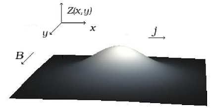
Figure 1: Interface between normal and superconducting regions in a type-I superconductor, pinned by a planar defect in the XY plane. Transport current parallel to the interface controls the energy barrier. Depinning of the interface occurs through quantum nucleation of a critical bump described by the instanton of the equations of motion in 2+1 dimensions.

Somewhat similar problems in 1+1 dimensions have been studied for a flux line pinned by the interlayer atomic potential in a layered superconductor Ivlev-1991 and for a flux line pinned by a columnar defect CD-1995 . However, the two-dimensional nature of the interface, as compared to a one-dimensional flux line, makes the interface problem more challenging. Note that tunneling of two-dimensional objects has been studied theoretically in application to non-thermal dynamics of planar domain walls Stamp and quantum nucleation of magnetic bubbles bubbles . These studies employed non-dissipative dynamics of the magnetization field because corrections coming from dissipation are not dominant for spin systems. On the contrary, the Euclidean dynamics of the interface in a type-I superconductor is entirely dissipative, described by integro-differential equations in 2+1 dimensions. As far as we know this problem has not been studied before.

The article is structured as follows. Theoretical model is formulated in Sec. II. Properties of the pinning potential and the effective action in the vicinity of the critical depinning current are analyzed in Sec. III. Instantons of the dissipative model in 2+1 dimensions are investigated in Sec. IV. Crossover from quantum tunneling to thermal activation is studied in Sec. V. Sec. VI contains estimates of the effect and final conclusions.

II The Model

We describe the interface by a smooth function $Z(x,y)$, see Fig. 1. Dimensionless Euclidean effective action associated with the interface is

$$S_{eff}=\frac{\sigma}{\hbar}\oint\,\mathrm{d}\tau\int\,\mathrm{d}x\,\mathrm{d}y\left[1+({\bm{\nabla}}Z)^{2}\right]^{\frac{1}{2}}$$

$$+\frac{1}{\hbar}\oint\,\mathrm{d}\tau\int\,\mathrm{d}x\,\mathrm{d}y\,V\left[x,y,Z(x,y,\tau)\right]$$ (1)

$$+\frac{\eta}{4\pi\hbar}\oint\,\mathrm{d}\tau\int_{\mathbf{R}}\,\mathrm{d}\tau^{\prime}\int\,\mathrm{d}x\,\mathrm{d}y\frac{\left[Z(x,y,\tau)-Z(x,y,\tau^{\prime})\right]^{2}}{(\tau-\tau^{\prime})^{2}}$$

where $\tau$ is the imaginary time, $\sigma$ is the surface energy density of the interface and $\eta$ is a drag coefficient, given respectively by LP ; Pb-tunneling

$$\sigma=\frac{B_{c}^{2}\xi}{3\sqrt{2}\pi}\,,\quad\eta=\frac{B_{c}^{2}\sqrt{\lambda_{L}\xi}}{2\rho_{n}c^{2}}\,,$$ (2)

with $B_{c}$ being the thermodynamic critical field, $\xi$ being the superconducting coherence length, $\lambda_{L}$ being the London length, and $\rho_{n}$ being the normal state resistivity. The first term in Eq. (II) is due to the elastic energy of the interface associated with its total area, the second term is due to the space-dependent potential energy, $V\left[x,y,Z(x,y)\right]$, of the interface inside the imperfect crystal, and the third term is due to dissipation Caldeira-Leggett . Same as for the flux lines, we neglect the inertial mass of the interface. Its dynamics in a type-I superconductor is dominated by friction.

We consider pinning of the interface by a planar defect located in the $XY$ plane and choose the pinning potential in the form

$$V_{p}=p\sigma\int\,\mathrm{d}x\,\mathrm{d}y\;\left(\frac{1}{2}\frac{Z^{2}}{a^{2}}-\frac{1}{4}\frac{Z^{4}}{a^{4}}\right)$$ (3)

where $2a$ is roughly the width of the well that traps the interface and $p\lesssim 1$ is a dimensionless constant describing the strength of the pinning. The interface separates the normal state at $Z<0$ from a superconducting state at $Z>0$. Superconducting current parallel to the planar defect (and to the interface pinned by the defect) exerts a Lorentz force on the interface similar to the force acting on a vortex line in a type-II superconductor. We shall assume that the magnetic field is applied in the $\hat{y}$ direction and that the transport current of density $j$ flows in the $\hat{x}$ direction. The driving force experienced by the $\mathrm{d}x\mathrm{d}y$ element of the interface in the $\hat{z}$ direction is given by

$$\frac{\mathrm{d}^{2}F_{z}}{\mathrm{d}x\mathrm{d}y}=\frac{1}{c}\int\,\mathrm{d}zjB(z)\,,$$ (4)

Here $B(z)=B_{c}\exp(-z/\delta)$ is the magnetic field inside the interface with $\delta=\sqrt{\xi\lambda_{L}}$. Integration then gives ${\mathrm{d}^{2}F_{z}}/({\mathrm{d}x\mathrm{d}y})={B_{c}\delta}j/c$. The corresponding contribution to the potential can be obtained by writing $F_{z}$ as $-\nabla_{Z}V_{L}$, yielding

$$\frac{\mathrm{d}^{2}V_{L}(Z)}{\mathrm{d}x\mathrm{d}y}=-\frac{B_{c}\delta}{c}jZ\,.$$ (5)

The total potential, $V(Z)=V_{p}(Z)+V_{L}(Z)$ is

$$V(Z)=p\sigma\int\,\mathrm{d}x\,\mathrm{d}y\left(-\bar{j}\tilde{Z}+\frac{\tilde{Z}^{2}}{2}-\frac{\tilde{Z}^{4}}{4}\right)$$ (6)

where we have introduced dimensionless $\tilde{Z}=Z/a$ and

$$\bar{j}=\frac{a\delta B_{c}}{pc\sigma}j=\frac{3\pi\sqrt{2{\kappa}}a}{pcB_{c}}j$$ (7)

with $\kappa=\lambda_{L}/\xi$. Note that for a type-I superconductor $\kappa<1/\sqrt{2}$.

III Effective Action in the Vicinity of the Critical Current

Measurable quantum depinning of the interface can occur only when the transport current is close to the critical current, $j_{c}$, that destroys the energy barrier. It is, therefore, makes sense to study the problem at $j\rightarrow j_{c}$. Maxima and minima of the function

$$f(\bar{j},\tilde{Z})=-\bar{j}\tilde{Z}+\frac{\tilde{Z}^{2}}{2}-\frac{\tilde{Z}^{4}}{4}$$ (8)

that enters Eq. (6) are given by the roots of the equation $\tilde{Z}^{3}-\tilde{Z}+\bar{j}=0$. At $j^{2}<4/27$ it has three real roots corresponding to one minimum and two maxima of the potential on two sides of the pinning layer, whereas at $j^{2}>4/27$ there is one real root corresponing to the maximum of $f$. Consequently, the barrier disappears at $j^{2}=4/27$, providing the value of the critical current

$$\bar{j}_{c}=\frac{2}{3\sqrt{3}}\,,\quad j_{c}=\frac{2pcB_{c}}{9\pi\sqrt{6\kappa}a}\,.$$ (9)

At $\bar{j}=\bar{j}_{c}$ the minimum and the maximum of the potential combine into the inflection point $\tilde{Z}=\tilde{Z}_{c}$ given by the set of equations

$$0 = -\tilde{Z}_{c}^{3}+\tilde{Z}_{c}-\bar{j}_{c}$$

$$0 = -3\tilde{Z}_{c}^{2}+1$$ (10)

that correspond to zero first and second derivatives of $f$. The value of $\tilde{Z}_{c}$ deduced from these equations is ${1}/{\sqrt{3}}$. It is convenient to introduce small parameter

$$\epsilon=1-{j}/{j_{c}}\,,$$ (11)

so that $j=j_{c}(1-\epsilon)$ and

$$\bar{j}=\bar{j}_{c}(1-\epsilon)=\frac{2}{3\sqrt{3}}(1-\epsilon)\,.$$ (12)

Let $\tilde{Z}_{0}(\bar{j})$ be the minimum of $f$ (see Fig. 2) satisfying

$$\tilde{Z}_{0}^{3}-\tilde{Z}_{0}+\bar{j}_{c}(1-\epsilon)=0\,.$$ (13)

Consider $\tilde{Z}^{\prime}=\tilde{Z}-\tilde{Z}_{0}$. It is easy to find that the form of the potential in the vicinity of $\tilde{Z}_{0}$ is

$$f=f[\tilde{Z}_{0}(\bar{j})]+\frac{1}{2}(1-3\tilde{Z}_{0}^{2})\tilde{Z}^{\prime 2}-\tilde{Z}_{0}\tilde{Z}^{\prime 3}-\frac{\tilde{Z}^{\prime 4}}{4}\,.$$ (14)

At small $\epsilon$ one has $\tilde{Z}_{0}\rightarrow\tilde{Z}_{c}=1/\sqrt{3}$, so that $1-3\tilde{Z}_{0}^{2}$ in front of $\tilde{Z}^{\prime 2}$ in Eq. (14) is small. The first term in Eq. (14) can be omitted as unessential shift of energy, while the last term proportional to $\tilde{Z}^{\prime 4}$ can be neglected due to its smallness compared to other $\tilde{Z}^{\prime}$-dependent terms. Consequently, one obtains the “effective potential”

$$f_{eff}(\bar{j},\tilde{Z})=\frac{1}{2}(1-3\tilde{Z}_{0}^{2})\tilde{Z}^{2}-\tilde{Z}_{0}\tilde{Z}^{3}\,.$$ (15)

We need to know the dependence of $\tilde{Z}_{0}$ on $\epsilon$. Writing $\tilde{Z}_{0}(\epsilon)=\tilde{Z}_{c}[1-\beta(\epsilon)]$, with the help of Eq. (13), we obtain $\displaystyle\beta(\epsilon)=\sqrt{2\epsilon/3}$ to the lowest order on $\epsilon$. Then $1-3\tilde{Z}_{0}^{2}\approx 2\sqrt{2\epsilon/3}$ and

$$f_{eff}(\epsilon,\tilde{Z})=\sqrt{\frac{2\epsilon}{3}}\tilde{Z}^{2}-\frac{\tilde{Z}^{3}}{\sqrt{3}}\,.$$ (16)

The height of the effective potential is $\displaystyle\frac{8}{27}\sqrt{\frac{2}{3}}\epsilon^{3/2}$ and the width is $\sqrt{2\epsilon}$, see Fig. 2.

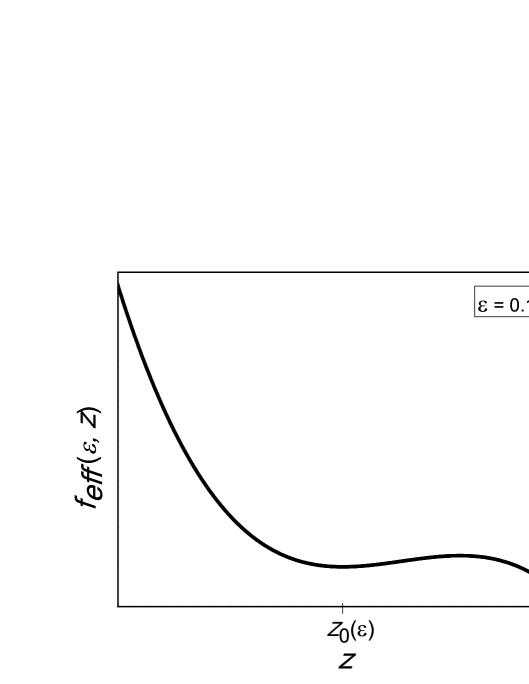
Figure 2: Effective potential

As follows from the equations of motion, smallness of ${\epsilon}$ results in $|{\bm{\nabla}}Z|\sim p\epsilon\ll 1$. This allows one to replace $\left[1+({\bm{\nabla}}Z)^{2}\right]^{\frac{1}{2}}$ in Eq. (II) with $1+\frac{1}{2}({\bm{\nabla}}Z)^{2}$. Introducing dimensionless variables

$$x_{0}=\left(\frac{2p\sqrt{\epsilon}}{3\sqrt{3}}\frac{\xi B_{c}^{2}}{\eta a^{2}}\right)\tau,\quad(x_{1},x_{2})=\left(\sqrt{2\epsilon/3}\;p\right)^{1/2}\frac{(x,y)}{a}$$

$$v=V(x,y,Z)/\sigma p,\quad u=\frac{3}{\sqrt{2\epsilon}}\left(Z/a-\tilde{Z}_{c}(1-\sqrt{2\epsilon/3})\right)$$

we obtain

$$S_{eff} = \frac{\sqrt{\epsilon}}{3\sqrt{6}\pi p}\frac{\eta a^{4}}{\hbar}\oint\,\mathrm{d}x_{0}\int\,\mathrm{d}x_{1}\,\mathrm{d}x_{2}\Bigg{[}\frac{1}{2}({\bm{\nabla}}u)^{2}+u^{2}-\frac{u^{3}}{3}$$ (18)

$$+ \frac{1}{2}\int_{\mathbf{R}}\,\mathrm{d}x_{0}^{\prime}\frac{\left[u(x_{0},x_{1},x_{2})-u(x_{0}^{\prime},x_{1},x_{2})\right]^{2}}{(x_{0}-x_{0}^{\prime})^{2}}\Bigg{]}$$

where $\nabla=(\partial_{1},\partial_{2})$.

IV Instantons of the Dissipative 2+1 Model

Quantum depinning of the interface is given by the instanton solution of the Euler-Lagrange equations of motion of the 2+1 field theory described by Eq. (18):

$$\sum_{\mu=0,1,2}\frac{\partial}{\partial x^{\mu}}\left[\frac{\delta\mathcal{L}}{\delta\left({\partial u}/{\partial x^{\mu}}\right)}\right]-\frac{\partial\mathcal{L}}{\partial u}=0\,.$$ (19)

This gives

$$\nabla^{2}u-2u+u^{2}-2\int_{\mathbf{R}}\,\mathrm{d}x_{0}^{\prime}\frac{u(x_{0},x_{1},x_{2})-u(x_{0}^{\prime},x_{1},x_{2})}{(x_{0}-x_{0}^{\prime})^{2}}=0$$ (20)

with the boundary conditions

$$u(-\Omega/2,x_{1},x_{2})=u(\Omega/2,x_{1},x_{2})\quad\forall(x_{1},x_{2})\in\mathbf{R}^{2}$$

$$\max_{x_{0}\in[-\Omega/2,\Omega/2]}u(x_{0},x_{1},x_{2})=u(0,x_{1},x_{2})\quad\forall(x_{1},x_{2})\in\mathbf{R}^{2}$$

that must be periodic on imaginary time with the period $\hbar/(k_{B}T)$. The corresponding period on $x_{0}$ is

$$\Omega=\left(\frac{2p\sqrt{\epsilon}}{3\sqrt{3}}\frac{\xi B_{c}^{2}}{\eta a^{2}}\right)\frac{\hbar}{k_{B}T}\,.$$ (22)

This equation cannot be solved analytically, so we must proceed by means of numerical methods.

IV.1 Zero temperature

We apply the Fourier transform

$$\hat{u}(\vec{\omega})=\frac{1}{(2\pi)^{3/2}}\int_{\mathbf{R}^{3}}u(\vec{x})e^{i\vec{\omega}\cdot\vec{x}}\,\mathrm{d}^{3}x$$ (23)

to equation (20) and get

$$\hat{u}(\vec{\omega})=\frac{(2\pi)^{-3/2}}{2+2\pi|\omega_{0}|+\omega_{1}^{2}+\omega_{2}^{2}}\int_{\mathbf{R}^{3}}\,\mathrm{d}^{3}\omega^{\prime}\hat{u}(\vec{\omega}-\vec{\omega}^{\prime})\hat{u}(\vec{\omega}^{\prime})$$ (24)

which is still an integral equation for $\hat{u}(\vec{\omega})$. The effective action (18) in terms of $\hat{u}(\vec{\omega})$ becomes

$$S_{eff}\left[\hat{u}\right]=\frac{\sqrt{\epsilon}}{3\sqrt{6}\pi p}\frac{\eta a^{4}}{\hbar}\Bigg{[}\int_{\mathbf{R}^{3}}\,\mathrm{d}^{3}\omega\;\hat{u}(\vec{\omega})\hat{u}(-\vec{\omega})\times$$

$$\Big{(}\frac{1}{2}(\omega_{1}^{2}+\omega_{2}^{2})+1+\pi|\omega_{0}|\Big{)}-$$

$$\frac{1}{3(2\pi)^{3/2}}\int_{\mathbf{R}^{6}}\,\mathrm{d}^{3}\omega\,\mathrm{d}^{3}\omega^{\prime}\hat{u}(\vec{\omega})\hat{u}(\vec{\omega}^{\prime})\hat{u}(-\vec{\omega}-\vec{\omega}^{\prime})\Bigg{]}.$$ (25)

We use the algorithm that is a field-theory extension of the algorithm introduced in Refs. Chang, ; Waxman, for the problem of dissipative quantum tunneling of a particle. It consists of the following steps:

1. Start with an initial aproximation $\hat{u}_{0}(\vec{\omega})$. Define the operator

   $$\hat{O}:\mathbf{R}\times\mathcal{L}^{2}(\mathbf{R}^{3})\rightarrow\mathcal{L}^{2}(\mathbf{R}^{3})$$ (26)

   $$(\lambda,\hat{u}(\vec{\omega}))\mapsto\displaystyle\frac{\lambda}{2+2\pi|\omega_{0}|+\omega_{1}^{2}+\omega_{2}^{2}}\int_{\mathbf{R}^{3}}\,\mathrm{d}^{3}\omega^{\prime}\hat{u}(\vec{\omega}-\vec{\omega}^{\prime})\hat{u}(\vec{\omega}^{\prime})$$

2. Let $\hat{u}_{1}(\vec{\omega})=\hat{O}(\lambda_{0},\hat{u}_{0}(\vec{\omega}))$ for an initial $\lambda_{0}\in\mathbf{R}$.

3. Calculate $\lambda_{1}=\lambda_{0}/\xi^{2}$ with $\xi=\frac{\hat{u}_{1}(\vec{\omega}=0)}{\hat{u}_{0}(\vec{\omega}=0)}$.

4. Find $\hat{u}_{2}(\vec{\omega})=\hat{O}(\lambda_{1},\hat{u}_{1}(\vec{\omega}))$.

5. Repeat steps $(2)-(4)$ until the successive difference satisfies a preset convergence criterion.

The output is the pair $(\lambda_{n},\hat{u}_{n}(\vec{\omega}))$. Finally, we apply a rescaling of $\hat{u}_{n}$ by a factor $\displaystyle(2\pi)^{3/2}\lambda_{n}$ to obtain the instanton solution. This procedure leads to

$$S_{eff}=\frac{\sqrt{\epsilon}}{3\sqrt{6}\pi p}\frac{\eta a^{4}}{\hbar}I_{0}$$ (27)

with numerical value of the integral $I_{0}=531\pm 19$. This somewhat surprisingly large value of the integral has been confirmed by our use of different computational grids.

IV.2 Non-zero temperature

At $T\neq 0$ the period of the instanton solution is finite, given by Eq. (22). We look for a solution of the type

$$u(x_{0},x_{1},x_{2})=\sum_{n\in\mathbf{Z}}e^{i\omega_{0,n}x_{0}}u_{n}(x_{1},x_{2})$$ (28)

with $\displaystyle\omega_{0,n}={2\pi n}/{\Omega}$. Introducing into (20) the above functional dependence and applying a 2D Fourier transform we obtain

$$\hat{u}_{n}(\vec{\omega})=\frac{1}{2+2\pi|\omega_{0,n}|+\vec{\omega}^{2}}\times$$

$$\left(\frac{1}{2\pi}\sum_{p\in\mathbf{Z}}\int_{\mathbf{R}^{2}}\,\mathrm{d}^{2}\omega^{\prime}\hat{u}_{n-p}(\vec{\omega}-\vec{\omega}^{\prime})\hat{u}_{p}(\vec{\omega}^{\prime})\right)\,,$$ (29)

which is the integral equation for $\hat{u}_{n}$ with $\vec{\omega}=(\omega_{1},\omega_{2})$. In terms of $\big{\{}\hat{u}_{n}(\vec{\omega})\big{\}}_{n}$ the effective action becomes

$$S_{eff}\left[\big{\{}\hat{u}\big{\}}_{n}\right]=\frac{\sqrt{\epsilon}}{3\sqrt{6}\pi p}\frac{\eta a^{4}}{\hbar}\times$$

$$\Bigg{[}\sum_{n\in\mathbf{Z}}\int_{\mathbf{R}^{2}}\,\mathrm{d}^{2}\omega\hat{u}_{n}(\vec{\omega})\hat{u}_{-n}(-\vec{\omega})\left(\frac{\vec{\omega}^{2}}{2}+1+\pi|\omega_{0,n}|\right)-$$

$$\frac{1}{6\pi}\sum_{n,m\in\mathbf{Z}}\int_{\mathbf{R}^{4}}\,\mathrm{d}^{2}\omega\,\mathrm{d}^{2}\omega^{\prime}\hat{u}_{n}(\vec{\omega})\hat{u}_{m}(\vec{\omega}^{\prime})\hat{u}_{-n-m}(-\vec{\omega}-\vec{\omega}^{\prime})\Bigg{]}\Omega$$

The numerical algorithm is analogous to the one used in the $T=0$ case. It leads to

$$S_{eff}=\frac{\sqrt{\epsilon}}{3\sqrt{6}\pi p}\frac{\eta a^{4}}{\hbar}I(T)$$ (31)

The value of the integral depends on the value of $T$ in comparison with the temperature, $T_{c}$, of the crossover from quantum tunneling to thermal activation (see below). At $T\ll T_{c}$ the numerical value of $I(T)$ is very close to $I_{0}$, while at $T\gg T_{c}$ we recover the Boltzmann exponent, $S_{eff}=V_{0}/(k_{B}T)$, with $V_{0}$ being the energy barrier for depinning. Computation of $I(T)$ in the intermediate temperature range requires very large computer time and will be reported elsewhere. Nevertheless, as we shall see below, the crossover temperature $T_{c}$ can be computed exactly.

V Crossover Temperature

The crossover temperature can be computed by means of theory of phase transitions Tc . Above $T_{c}$, the solution minimizing the instantion action is a function $u(x_{0},x_{1},x_{2})=\bar{u}_{0}(x_{1},x_{2})$ that does not depend on $x_{0}$. Just below $T_{c}$, the instanton solution can be split into the sum of $\bar{u}_{0}$ and a term that depends $x_{0}$,

$$u(x_{0},x_{1},x_{2})=\bar{u}_{0}(x_{1},x_{2})+u_{1}(x_{1},x_{2})\cos(2\pi/\Omega x_{0})\,.$$ (32)

The instanton action is proportional to

$$\int_{\mathbb{R}^{2}}\,\mathrm{d}x_{1}\,\mathrm{d}x_{2}\Phi(x_{1},x_{2};u,\nabla u)\,,$$ (33)

where $\Phi(x_{1},x_{2};u,\nabla u)$ is the spatial action density. Using the expansion of $u$ introduced in the previous section, we obtain

$$\Phi(x_{1},x_{2};u_{1},\nabla u_{1})=\Omega\left[\frac{1}{2}(\nabla\bar{u}_{0})^{2}+v(\bar{u}_{0})\right]+$$

$$\frac{\Omega}{4}(\nabla u_{1})^{2}+\Lambda u_{1}^{2}+O(4)$$ (34)

with $\displaystyle v(u)=u^{2}-{u^{3}}/{3}$ and

$$\Lambda=\frac{\Omega}{4}v^{\prime\prime}(\bar{u}_{0})+\pi^{2}\,.$$ (35)

If $\Lambda>0$, the only $(u_{1},\nabla u_{1})$ minimizing $\Phi$ is $u_{1}\equiv 0$, so we define the crossover temperature by the equation

$$\min_{\vec{x}\in\mathbb{R}^{2}}\Lambda=\min_{\vec{x}\in\mathbb{R}^{2}}\frac{\Omega_{c}}{4}v^{\prime\prime}[\bar{u}_{0}(x_{1},x_{2})]+\pi^{2}=0\,.$$ (36)

Notice that this minimum corresponds to the minimum of $v^{\prime\prime}[\bar{u}_{0}(x_{1},x_{2}))]$. The equation of motion for $\bar{u}_{0}$ is

$$\nabla^{2}\bar{u}_{0}-2\bar{u}_{0}+\bar{u}_{0}^{2}=0\,.$$ (37)

Solution corresponding to the minimum is spherically symmetric,

$$\bar{u}_{0}=\bar{u}_{0}\left(r=\sqrt{x_{1}^{2}+x_{2}^{2}}\right)\,,$$ (38)

satisfying boundary conditions: $\bar{u}_{0}\rightarrow 0$ at $r\rightarrow\infty$ and $\bar{u}_{0}(0)=3$, which is the width of the potential. Consequently,

$$\min_{\vec{x}\in\mathbb{R}^{2}}v^{\prime\prime}[\bar{u}_{0}(x_{1},x_{2})]=\min_{\bar{u}_{0}\in[0,3]}v^{\prime\prime}(\bar{u}_{0})$$

$$=\min_{\bar{u}_{0}\in[0,3]}2(1-\bar{u}_{0})=-4\,.$$ (39)

Then, according to equations (35) and (36), the crossover temperature is determined by the equation $\Omega(T_{c})=\pi^{2}$, which gives

$$T_{c}=\frac{2p\sqrt{\epsilon}}{3\sqrt{3}\pi^{2}}\frac{\hbar\xi B_{c}^{2}}{k_{B}\eta a^{2}}=\frac{4p\sqrt{\epsilon}}{3\pi^{2}\sqrt{3\kappa}}\frac{\hbar\rho_{n}c^{2}}{k_{B}a^{2}}\,.$$ (40)

VI Discussion

We are now in a position to discuss feasibility of the proposed experiment on quantum depinning of the interface from a planar defect in a type-I superconductor. Two conditions must be satisfied. Firstly the dimensionless effective action of Eq. (27), which is the WKB exponent of the tunneling rate, should not exceed $30-40$ in order for the tunneling to occur on a reasonable time scale. Secondly, the crossover temperature determined by Eq. (40) better be not much less than one kelvin. For a known superconductor, the two equations contain three parameters: The parameter $p\leq 1$ describing the strength of pinning, the parameter $a$ describing the width of the pinning layer, and the parameter $\epsilon$ that controls how close the transport current should be to the depinning current. We, therefore, have to investigate how practical is the range of values of these parameters that can provide conditions $S_{eff}\sim 30$ and $T_{c}\sim 1$K.

Let us choose lead as an example. The values of $\lambda_{L}$ and $\xi$ in lead are $37\,$nm and $38\,$nm, respectively, giving $\kappa=\lambda_{L}/\xi=0.45$. The critical field is $B_{c}\approx 800\,$G. The elastic energy of the interface is $\sigma\approx 0.4\,$erg/cm². The normal state resistivity in the kelvin range is $5\times 10^{-11}$ $\Omega\cdot$m = $5.6\times 10^{-21}$s., while the drag coefficient is $\eta\approx 0.35\,$erg$\cdot$s/cm⁴. Then equations (27) and (40) with conditions $S_{eff}\sim 30$ and $T_{c}\sim 1$K give $a/p^{1/3}\sim 3.7\,$nm and $\sqrt{\epsilon}a\sim 0.25\,$nm. If the pinning layer is incompatible with superconductivity, then at $2a<\xi$ one should expect $p\sim 2a/\xi$, giving $a\sim 1.65\,$nm and $\epsilon\sim 0.02$. This means that observation of quantum escape of the interface from a pinning layer of thickness $2a\sim 3.3\,$nm in a superconducting Pb sample at $T\sim 1\,$K would require control of the transport current within two percent of the critical depinning current. All the above parameters are within experimental reach.

In conclusion, we have studied quantum escape from a planar pinning defect of the interface separating superconducting and normal regions in a type-I superconductor. This can correspond to either quantum depinning of the interface from a grain boundary or quantum depinning from an artificially prepared layer. The computed tunneling rate, the required temperature and other parameters all fall within realistic experimental range. We encourage such experiment as it would present a rare opportunity to study, in a controllable manner, dissipative quantum tunneling of an extended object.

VII Acknoweledgements

The work at the University of Barcelona has been supported by the Spanish Government project No. MAT2008-04535 and by Catalan ICREA Academia. R.Z. acknowledges financial support from the Ministerio de Ciencia e Innovación de España. The work of E.M.C. at Lehman College has been supported by the U.S. Department of Energy through grant No. DE-FG02-93ER45487.

References

(1)
A. O. Caldeira and A. J. Leggett, Phys. Rev. Lett. 46, 211
(1981); Ann. Phys. (N.Y.) 149, 374 (1983).
(2)
J. Clarke, A. N. Cleland, M. H. Devoret, D. Esteve, and J. M.
Martinis, Science 239, 992 (1988).
(3)
E. M. Chudnovsky and J. Tejada, Macroscopic Quantum Tunneling
of the Magnetic Moment (Cambridge University Press, Cambridge,
England, 1998).
(4)
G. Blatter, M. V. Feigel’man, V. B. Geshkenbein, A. I. Larkin, and
V. M. Vinokur, Rev. Mod. Phys. 66, 1125 (1994).
(5)
Y. Yeshurun, A. P. Malozemoff, A. Shaulov, Rev. Mod. Phys. 68, 911 (1996).
(6)
T. Nattermann and S. Scheidl, Adv. Phys. 49, 607 (2000).
(7)
E. M. Chudnovsky, O. Iglesias, and P. C. E. Stamp, Phys. Rev. B
46, 5392 (1992).
(8)
K. Hong and N. Giordano, J. Phys.: Cond. Matter 8, L301
(1996).
(9)
J. Brooke, T. F. Rosenbaum, and G. Aeppli, Nature 413, 610
(2001).
(10)
G. Blatter, V. B. Geshkenbein, and V. M. Vinokur, Phys. Rev. Lett.
66, 3297 (1991).
(11)
B. I. Ivlev, Yu. M. Ovchinnikov, R. S. Thompson, Phys. Rev. B 44, 7023 (1991).
(12)
J. Tejada, E. M. Chudnovsky, and A. Garcia, Phys. Rev. B 47,
11552 (1993).
(13)
P. Ao and D. J. Thouless, Phys. Rev. Lett. 72, 132 (1994).
(14)
M. J. Stephen, Phys. Rev. Lett. 72, 1534 (1994).
(15)
E. M. Chudnovsky, S. Vélez, A. García-Santiago, J. M.
Hernandez, and J. Tejada, Phys. Rev. B 83, 064507 (2011).
(16)
L. D. Landau, Phys. Z. Sowjetunion 11, 129 (1937).
(17)
Y. V. Sharvin, Zh. Eksp. Teor. Fiz. 33, 1341 (1957).
(18)
R. P. Huebener, Magnetic Flux Structures of Superconductors
( Springer-Verlag, New York, 1990).
(19)
A. V. Kuznetsov, D. V. Eremenko, and V. N. Trofimov, Phys. Rev. B
57, 5412 (1998).
(20)
A. Cebers, C. Gourdon, V. Jeudy, and T. Okada, Phys. Rev. B 72, 014513 (2005).
(21)
M. Menghini and R. J. Wijngaarden, Phys. Rev. B 72, 172503
(2005).
(22)
R. Prozorov, Phys. Rev. Lett. 98, 257001 (2007).
(23)
R. Prozorov, A. F. Fidler, J. R. Hoberg, and P. C. Canfield,
Nature Physics 4, 327 (2008).
(24)
S. Vélez, A. García-Santiago, J. M. Hernandez, and J.
Tejada, Phys. Rev. B 80, 144502 (2009).
(25)
E. M. Chudnovsky, A. Ferrera, and A. Vilenkin, Phys. Rev. B 51, 1181 (1995).
(26)
E. M. Chudnovsky and L. Gunther, Phys. Rev. B 37, 9455
(1988); A. Ferrera and E. M. Chudnovsky, Phys. Rev. B 53,
354 (1996).
(27)
E. M. Lifshitz and L. P. Pitaevskii, Statistical Physics,
Part 2 (Oxford: Pergamon, 1980).
(28)
L. Chang and S. Chakravarty, Phys. Rev. B 29, 130 (1984).
(29)
D. Waxman and A. J. Leggett, Phys. Rev. B 32, 4450 (1985).
(30)
I. Affieck, Phys. Rev. Lett. 46, 388 (1981); A. I. Larkin
and Yu. N. Ovchinnikov, Pis’ma Zh. Eksp. Teor. Fiz. 37, 322
(1983) [JETP 37, 382 (1983)]; E. M. Chudnovsky, Phys. Rev. A 46, 8011 (1992).