Solving Principal Component Pursuit in Linear Time via $l_{1}$ Filtering

Abstract

In the past decades, exactly recovering the intrinsic data structure from corrupted observations, which is known as robust principal component analysis (RPCA), has attracted tremendous interests and found many applications in computer vision. Recently, this problem has been formulated as recovering a low-rank component and a sparse component from the observed data matrix. It is proved that under some suitable conditions, this problem can be exactly solved by principal component pursuit (PCP), i.e., minimizing a combination of nuclear norm and $l_{1}$ norm. Most of the existing methods for solving PCP require singular value decompositions (SVD) of the data matrix, resulting in a high computational complexity, hence preventing the applications of RPCA to very large scale computer vision problems. In this paper, we propose a novel algorithm, called $l_{1}$ filtering, for exactly solving PCP with an $O(r^{2}(m+n))$ complexity, where $m\times n$ is the size of data matrix and $r$ is the rank of the matrix to recover, which is supposed to be much smaller than $m$ and $n$. Moreover, $l_{1}$ filtering is highly parallelizable. It is the first algorithm that can exactly solve a nuclear norm minimization problem in linear time (with respect to the data size). Experiments on both synthetic data and real applications testify to the great advantage of $l_{1}$ filtering in speed over state-of-the-art algorithms.

1 Introduction

Robustly recovering the intrinsic low-dimensional structure of high-dimensional visual data, which is known as robust principal component analysis (RPCA), plays a fundamental role in various computer vision tasks, such as face image alignment and processing, video denoising, structure from motion, background modeling, photometric stereo and texture representation (see e.g., Wright et al (2009), Ji et al (2010), De la Torre and Black (2003), Peng et al (2010), Wu et al (2010), and Zhang et al (2012), to name just a few). Through the years, a large number of approaches have been proposed for solving this problem. The representative works include De la Torre and Black (2003), Nie et al (2011), Aanes et al (2002), Baccini et al (1996), Ke and Kanade (2005), Skocaj et al (2007), and Storer et al (2009). The main limitation of above mentioned methods is that there is no theoretical guarantee for their performance. Recently, the advances in compressive sensing have led to increasingly interests in considering RPCA as a problem of exactly recovering a low-rank matrix $\mathbf{L}_{0}$ from corrupted observations $\mathbf{M}=\mathbf{L}_{0}+\mathbf{S}_{0}$, where $\mathbf{S}_{0}$ is known to be sparse (Wright et al (2009), Candés et al (2011)). Its mathematical model is as follows:

$$\min\mbox{rank}(\mathbf{L})+\lambda\|\mathbf{S}\|_{l_{0}},\quad s.t.\quad\mathbf{M}=\mathbf{L}+\mathbf{S},$$ (1)

where $\|\cdot\|_{l_{0}}$ is the $l_{0}$ norm of a matrix, i.e., the number of nonzero entries in the matrix.

Unfortunately, problem (1) is known to be NP-hard. So Candés et al (2011) proposed using principal component pursuit (PCP) to solve (1), which is to replace the rank function and $l_{0}$ norm with the nuclear norm (which is the sum of the singular values of a matrix, denoted as $\|\cdot\|_{*}$) and $l_{1}$ norm (which is the sum of the absolute values of the entries), respectively. More specifically, PCP is to solve the following convex problem instead:

$$\min\|\mathbf{L}\|_{*}+\lambda\|\mathbf{S}\|_{l_{1}},\quad s.t.\quad\mathbf{M}=\mathbf{L}+\mathbf{S}.$$ (2)

They also rigorously proved that under fairly general conditions and $\lambda=1/\sqrt{\max(m,n)}$, PCP can exactly recover the low-rank matrix $\mathbf{L}_{0}$ (namely the underlying low-dimensional structure) with an overwhelming probability, i.e., the difference of the probability from 1 decays exponentially when the matrix size increases. This theoretical analysis makes PCP distinct from previous methods for RPCA.

All the existing algorithms for RPCA need to compute either SVD or matrix-matrix multiplications on the whole data matrix. So their computation complexities are all at least quadratic w.r.t. the data size, preventing the applications of RPCA to large-scale problems when the time is critical. In this paper, we address the large-scale RPCA problem and propose a truly linear cost method to solve the PCP model (2) when the data size is very large while the target rank is relatively small. Such kind of data is ubiquitous in computer vision.

1.1 Main Idea

Our algorithm fully utilizes the properties of low-rankness. The main idea is to apply PCP to a randomly selected submatrix of the original noisy matrix and compute a low rank submatrix. Using this low rank submatrix, the true low rank matrix can be estimated efficiently, where the low rank submatrix is part of it.

Specifically, our method consists of two steps (illustrated in Figure 1). The first step is to recover a submatrix $\mathbf{L}^{s}$ (Figure 1 (e)) of $\mathbf{L}_{0}$. We call this submatrix the seed matrix because all other entries of $\mathbf{L}_{0}$ can be further calculated by this submatrix. The second step is to use the seed matrix to recover two submatrices $\mathbf{L}^{c}$ and $\mathbf{L}^{r}$ (Figures 1 (f)-(g)), which are on the same rows and columns as $\mathbf{L}^{s}$ in $\mathbf{L}_{0}$, respectively. They are recovered by minimizing the $l_{1}$ distance from the subspaces spanned by the columns and rows of $\mathbf{L}^{s}$, respectively. Hence we call this step $l_{1}$ filtering. The remaining part $\tilde{\mathbf{L}}_{s}$ (Figure 1 (h)) of $\mathbf{L}_{0}$ can be represented by $\mathbf{L}^{s}$, $\mathbf{L}^{c}$ and $\mathbf{L}^{r}$, using the generalized Nyström method (Wang et al (2009)). As analyzed in Section 3.4, our method is of linear cost with respect to the data size. Besides the advantage of linear time cost, the proposed algorithm is also highly parallel: the columns of $\mathbf{L}^{c}$ and the rows of $\mathbf{L}^{r}$ can be recovered fully independently. We also prove that under suitable conditions, our method can exactly recover the underling low-rank matrix $\mathbf{L}_{0}$ with an overwhelming probability. To our best knowledge, this is the first algorithm that can exactly solve a nuclear norm minimization problem in linear time.

(a) $\mathbf{M}$	(b) $\mathbf{L}_{0}$	(c) $\mathbf{S}_{0}$	(d) $\mathbf{L}^{*}$
(e) $\mathbf{L}^{s}$	(f) $\mathbf{L}^{c}$	(g) $\mathbf{L}^{r}$	(h) $\tilde{\mathbf{L}}^{s}$

Figure 1: Illustration of the proposed $l_{1}$ filtering method. A large observed data matrix $\mathbf{M}$ (a) is the sum of a low-rank matrix $\mathbf{L}_{0}$ (b) and a sparse matrix $\mathbf{S}_{0}$ (c). The method first recovers a seed matrix (a submatrix of $\mathbf{L}_{0}$) $\mathbf{L}^{s}$ (e). Then the submatrices $\mathbf{L}^{c}$ (f) and $\mathbf{L}^{r}$ (g) can be recovered by column and row filtering, respectively, where $\mathbf{U}$ and $\mathbf{V}^{T}$ are the column space and row space of $\mathbf{L}^{s}$, respectively. Then the complement matrix $\tilde{\mathbf{L}}^{s}$ (h) can be represented by $\mathbf{L}^{s}$, $\mathbf{L}^{c}$ and $\mathbf{L}^{r}$. Finally, we obtain the computed low-rank matrix $\mathbf{L}^{*}$ (d), which is identical to $\mathbf{L}_{0}$ with an overwhelming probability.

2 Previous Works

In this section, we review some previous algorithms for solving PCP. The existing solvers can be roughly divided into three categories: classic convex optimization, factorization and compressed optimization.

For small sized problems, PCP can be reformulated as a semidefinite program and then be solved by standard interior point methods. However, this type of methods cannot handle even moderate scale matrices due to their $O(n^{6})$ complexity in each iteration. So people turned to first-order algorithms, such as the dual method (Ganesh et al (2009)), the accelerated proximal gradient (APG) method (Ganesh et al (2009)) and the alternating direction method (ADM) (Lin et al (2009)), among which ADM is the most efficient. All these methods require solving the following kind of subproblem in each iteration

$$\min\limits_{\mathbf{A}}\eta\|\mathbf{A}\|_{*}+\frac{1}{2}\|\mathbf{A}-\mathbf{W}\|_{F}^{2},$$ (3)

where $\|\cdot\|_{F}$ is the Frobenious norm. Cai et al (2010) proved that the above problem has a closed form solution

$$\mathbf{A}=\mathbf{U}\mathcal{S}_{\eta}(\mathbf{\Sigma})\mathbf{V}^{T},$$ (4)

where $\mathbf{U}\mathbf{\Sigma}\mathbf{V}^{T}$ is the singular value decomposition of $\mathbf{W}$ and $\mathcal{S}_{\eta}(x)=\mbox{sgn}(x)\max(|x|-\eta,0)$ is the soft shrinkage operator. Therefore, these methods all require computing SVDs for some matrices, resulting in $O(mn\min(m,n))$ complexity, where $m\times n$ is the matrix size.

As the most expensive computational task required by solving (2) is to perform SVD, Lin et al (2009) adopted partial SVD (Larsen (1998)) to reduce the complexity at each iteration to $O(rmn)$, where $r$ is the target rank. However, such a complexity is still too high for very large data sets. Drineas et al (2006) developed a fast Monte Carlo algorithm, named linear time SVD (LTSVD), which can be used for solving SVDs approximately (also see Halko et al (2011)). The main drawback of LTSVD is that it is less accurate than the standard SVD as it uses random sampling. So the whole algorithm needs more iterations to achieve the same accuracy. As a consequence, the speed performance of LTSVD quickly deteriorates when the target rank increases (see Figure 2). Actually, even adopting LTSVD the whole algorithm is still quadratic w.r.t. the data size because it still requires matrix-matrix multiplication in each iteration.

To address the scalability issue of solving large-scale PCP problems, Shen et al (2011) proposed a factorization based method, named low-rank matrix fitting (LMaFit). This approach represents the low-rank matrix as a product of two matrices and then minimizes over the two matrices alternately. Although they do not require nuclear norm minimization (hence the SVDs), the convergence of the proposed algorithm is not guaranteed as the corresponding problem is non-convex. Moreover, both the matrix-matrix multiplication and the QR decomposition based rank estimation technique require $O(rmn)$ complexity. So this method does not essentially reduce the complexity.

Inspired by compressed optimization, Mu et al (2011) proposed reducing the problem scale by random projection (RP). However, this method is highly unstable – different random projections may lead to radically different results. Moreover, the need to introduce additional constraint to the problem slows down the convergence. And actually, the complexity of this method is also $O(pmn)$, where $p\times m$ is the size of the random projection matrix and $p>r$. So this method is still not of linear complexity with respect to the matrix size.

3 The $l_{1}$ Filtering Algorithm

Given an observed data matrix $\mathbf{M}\in\mathbb{R}^{m\times n}$, which is the sum of a low-rank matrix $\mathbf{L}_{0}$ and a sparse matrix $\mathbf{S}_{0}$, PCP is to recover $\mathbf{L}_{0}$ from $\mathbf{M}$. What our approach differs from traditional ones is that the underlying low-rank matrix $\mathbf{L}_{0}$ is reconstructed from a seed matrix. As explained in Section 1.1, our $l_{1}$ filtering algorithm consists of two steps: first recovering a seed matrix, second performing $l_{1}$ filtering on corresponding rows and columns of the data matrix. Below we provide details of these two steps.

3.1 Seed Matrix Recovery

Suppose that the target rank $r$ is very small compared with the data size: $r\ll\min(m,n)$. We first randomly sample an $(s_{r}r)\times(s_{c}r)$ submatrix $\mathbf{M}^{s}$ from $\mathbf{M}$, where $s_{r}>1$ and $s_{c}>1$ are the row and column oversampling rates, respectively. Then the submatrix $\mathbf{L}^{s}$ of the underlying matrix $\mathbf{L}_{0}$ can be recovered by solving a small sized PCP problem:

$$\min\limits_{\mathbf{L}^{s},\mathbf{S}^{s}}\|\mathbf{L}^{s}\|_{*}+\tilde{\lambda}\|\mathbf{S}^{s}\|_{l_{1}},\quad s.t.\quad\mathbf{M}^{s}=\mathbf{L}^{s}+\mathbf{S}^{s},$$ (5)

e.g., using ADM (Lin et al (2009)), where $\tilde{\lambda}=1/\sqrt{\max(s_{r}r,s_{c}r)}$.

By Theorem 1.1 in (Candés et al (2011)), the seed matrix $\mathbf{L}^{s}$ can be exactly recovered from $\mathbf{M}^{s}$ with an overwhelming probability when $s_{r}$ and $s_{c}$ increases. In fact, by that theorem $s_{r}$ and $s_{c}$ should be chosen at the scale of $O(\ln^{2}r)$. For the experiments conducted in this paper, whose $r$’s are very small, we simply choose $s_{c}=s_{r}=10$.

3.2 $l_{1}$ Filtering

For ease of illustration, we assume that $\mathbf{M}^{s}$ is the top left $(s_{r}r)\times(s_{c}r)$ submatrix of $\mathbf{M}$. Then accordingly $\mathbf{M}$, $\mathbf{L}_{0}$ and $\mathbf{S}_{0}$ can be partitioned into:

$$\mathbf{M}=\begin{bmatrix}\mathbf{M}^{s}&\mathbf{M}^{c}\\ \mathbf{M}^{r}&\tilde{\mathbf{M}}^{s}\end{bmatrix},\ \mathbf{L}_{0}=\begin{bmatrix}\mathbf{L}^{s}&\mathbf{L}^{c}\\ \mathbf{L}^{r}&\tilde{\mathbf{L}}^{s}\end{bmatrix},\ \mathbf{S}_{0}=\begin{bmatrix}\mathbf{S}^{s}&\mathbf{S}^{c}\\ \mathbf{S}^{r}&\tilde{\mathbf{S}}^{s}\end{bmatrix}.$$ (6)

Since $\mbox{rank}(\mathbf{L}_{0})=\mbox{rank}(\mathbf{L}^{s})=r$, there must exist matrices $\mathbf{Q}$ and $\mathbf{P}$, such that

$$\mathbf{L}^{c}=\mathbf{L}^{s}\mathbf{Q}\quad\mbox{and}\quad\mathbf{L}^{r}=\mathbf{P}^{T}\mathbf{L}^{s}.$$ (7)

As $\mathbf{S}_{0}$ is sparse, so are $\mathbf{S}^{c}$ and $\mathbf{S}^{r}$. Therefore, $\mathbf{Q}$ and $\mathbf{P}$ can be found by solving the following problems:

$$\min\limits_{\mathbf{S}^{c},\mathbf{Q}}\|\mathbf{S}^{c}\|_{l_{1}},\quad s.t.\quad\mathbf{M}^{c}=\mathbf{L}^{s}\mathbf{Q}+\mathbf{S}^{c},$$ (8)

and

$$\min\limits_{\mathbf{S}^{r},\mathbf{P}}\|\mathbf{S}^{r}\|_{l_{1}},\quad s.t.\quad\mathbf{M}^{r}=\mathbf{P}^{T}\mathbf{L}^{s}+\mathbf{S}^{r},$$ (9)

respectively. The above two problems can be easily solved by ADM.

With $\mathbf{Q}$ and $\mathbf{P}$ computed, $\mathbf{L}^{c}$ and $\mathbf{L}^{r}$ are obtained as (7). Again by $\mbox{rank}(\mathbf{L}_{0})=\mbox{rank}(\mathbf{L}^{s})=r$, the generalized Nyström method (Wang et al (2009)) gives:

$$\tilde{\mathbf{L}}^{s}=\mathbf{L}^{r}(\mathbf{L}^{s})^{\dagger}\mathbf{L}^{c},$$ (10)

where $(\mathbf{L}^{s})^{\dagger}$ is the Moore-Penrose pseudo inverse of $\mathbf{L}^{s}$.

In real computation, as the SVD of $\mathbf{L}^{s}$ is readily available when solving (5), due to the singular value thresholding operation (4), it is more convenient to reformulate (8) and (9) as

$$\min\limits_{\mathbf{S}^{c},\tilde{\mathbf{Q}}}\|\mathbf{S}^{c}\|_{l_{1}},\quad s.t.\quad\mathbf{M}^{c}=\mathbf{U}^{s}\tilde{\mathbf{Q}}+\mathbf{S}^{c},$$ (11)

and

$$\min\limits_{\mathbf{S}^{r},\tilde{\mathbf{P}}}\|\mathbf{S}^{r}\|_{l_{1}},\quad s.t.\quad\mathbf{M}^{r}=\tilde{\mathbf{P}}^{T}(\mathbf{V}^{s})^{T}+\mathbf{S}^{r},$$ (12)

respectively, where $\mathbf{U}^{s}\mathbf{\Sigma}^{s}(\mathbf{V}^{s})^{T}$ is the skinny SVD of $\mathbf{L}^{s}$ obtained from (4) in the iterations. Such a reformulation has multiple advantages. First, as $(\mathbf{U}^{s})^{T}\mathbf{U}^{s}=(\mathbf{V}^{s})^{T}\mathbf{V}^{s}=\mathbf{I}$, it is unnecessary to compute the inverse of $(\mathbf{U}^{s})^{T}\mathbf{U}^{s}$ and $(\mathbf{V}^{s})^{T}\mathbf{V}^{s}$ when updating $\tilde{\mathbf{Q}}$ and $\tilde{\mathbf{P}}$ in the iterations of ADM. Second, computing (10) also becomes easy if one wants to form $\tilde{\mathbf{L}}^{s}$ explicitly because now

$$\tilde{\mathbf{L}}^{s}=\tilde{\mathbf{P}}^{T}(\mathbf{\Sigma}^{s})^{-1}\tilde{\mathbf{Q}}.$$ (13)

To make the algorithm description complete, we sketch in Algorithm 1 the ADM for solving (11) and (12), which are both of the following form:

$$\min\limits_{\mathbf{E},\mathbf{Z}}\|\mathbf{E}\|_{l_{1}},\quad s.t.\quad\mathbf{X}=\mathbf{A}\mathbf{Z}+\mathbf{E},$$ (14)

where $\mathbf{X}$ and $\mathbf{A}$ are known matrices and $\mathbf{A}$ has orthonormal columns, i.e., $\mathbf{A}^{T}\mathbf{A}=\mathbf{I}$. The ADM for (14) is to minimize on the following augmented Lagrangian function

$$\|\mathbf{E}\|_{l_{1}}+\langle\mathbf{Y},\mathbf{X}-\mathbf{A}\mathbf{Z}-\mathbf{E}\rangle+\frac{\beta}{2}\|\mathbf{X}-\mathbf{A}\mathbf{Z}-\mathbf{E}\|_{F}^{2},$$ (15)

with respect to $\mathbf{E}$ and $\mathbf{Z}$, respectively, by fixing other variables, and then update the Lagrange multiplier $\mathbf{Y}$ and the penalty parameter $\beta$.

Algorithm 1 Solving (14) by ADM

  Input: $\mathbf{X}$ and $\mathbf{A}$.

  Initialize: Set $\mathbf{E}_{0}$, $\mathbf{Z}_{0}$ and $\mathbf{Y}_{0}$ to zero matrices. Set $\varepsilon>0$, $\rho>1$ and $\bar{\beta}\gg\beta_{0}>0$.

  while $\|\mathbf{X}-\mathbf{A}\mathbf{Z}_{k}-\mathbf{E}_{k}\|_{l_{\infty}}/\|\mathbf{X}\|_{l_{\infty}}\geq\varepsilon$ do

     Step 1: Update $\mathbf{E}_{k+1}=\mathcal{S}_{\beta_{k}^{-1}}(\mathbf{X}-\mathbf{A}\mathbf{Z}_{k}+\mathbf{Y}_{k}/\beta_{k}$), where $\mathcal{S}$ is the soft-thresholding operator (Cai et al (2010)).

     Step 2: Update $\mathbf{Z}_{k+1}=\mathbf{A}^{T}(\mathbf{X}-\mathbf{E}_{k+1}+\mathbf{Y}_{k}/\beta_{k})$.

     Step 3: Update $\mathbf{Y}_{k+1}=\mathbf{Y}_{k}+\beta_{k}(\mathbf{X}-\mathbf{A}\mathbf{Z}_{k+1}-\mathbf{E}_{k+1})$ and $\beta_{k+1}=\min(\rho\beta_{k},\bar{\beta})$.

  end while

Note that it is easy to see that (11) and (12) can also be solved in full parallelism as the columns and rows of $\mathbf{L}^{c}$ and $\mathbf{L}^{r}$ can computed independently, thanks to the decomposability of the problems. So the recovery of $\mathbf{L}^{c}$ and $\mathbf{L}^{r}$ is very efficient if one has a parallel computing platform, such as a general purpose graphics processing unit (GPU).

3.3 The Complete Algorithm

Now we are able to summarize in Algorithm 2 our $l_{1}$ filtering method for solving PCP, where steps 3 and 4 can be done in parallel.

Algorithm 2 The $l_{1}$ Filtering Method for Solving PCP (2)

  Input: Observed data matrix $\mathbf{M}$.

  Step 1: Randomly sample a submatrix $\mathbf{M}^{s}$.

  Step 2: Solve the small sized PCP problem (5), e.g., by ADM, to recover the seed matrix $\mathbf{L}^{s}$.

  Step 3: Reconstruct $\mathbf{L}^{c}$ by solving (11).

  Step 4: Reconstruct $\mathbf{L}^{r}$ by solving (12).

  Step 5: Represent $\tilde{\mathbf{L}}^{s}$ by (13).

  Output: Low-rank matrix $\mathbf{L}$ and sparse matrix $\mathbf{S}=\mathbf{M}-\mathbf{L}$.

3.4 Complexity Analysis

Now we analyze the computational complexity of the proposed Algorithm 2. For the step of seed matrix recovery, the complexity of solving (5) is only $O(r^{3})$. For the $l_{1}$ filtering step, it can be seen that the complexity of solving (11) and (12) is $O(r^{2}n)$ and $O(r^{2}m)$, respectively. So the total complexity of this step is $O(r^{2}(m+n))$. As the remaining part $\tilde{\mathbf{L}}_{s}$ of $\mathbf{L}_{0}$ can be represented by $\mathbf{L}^{s}$, $\mathbf{L}^{c}$ and $\mathbf{L}^{r}$, using the generalized Nyström method (Wang et al (2009)) and recall that $r\ll\min(m,n)$, we conclude that the overall complexity of Algorithm 2 is $O(r^{2}(m+n))$, which is only of linear cost with respect to the data size.

3.5 Exact Recoverability of $l_{1}$ Filtering

The exact recoverability of $\mathbf{L}_{0}$ using our $l_{1}$ filtering method consists of two factors. First, exactly recovering $\mathbf{L}^{s}$ from $\mathbf{M}^{s}$. Second, exactly recovering $\mathbf{L}^{c}$ and $\mathbf{L}^{r}$. If all $\mathbf{L}^{s}$, $\mathbf{L}^{c}$, and $\mathbf{L}^{r}$ can be exactly recovered, $\mathbf{L}_{0}$ is exactly recovered.

The exact recoverability of $\mathbf{L}^{s}$ from $\mathbf{M}^{s}$ is guaranteed by Theorem 1.1 of (Candés et al (2011)). When $s_{r}$ and $s_{c}$ are sufficiently large, the chance of success is overwhelming.

To analyze the exact recoverability of $\mathbf{L}^{c}$ and $\mathbf{L}^{r}$, we first observe that it is equivalent to the exact recoverability of $\mathbf{S}^{c}$ and $\mathbf{S}^{r}$. By multiplying annihilation matrices $\mathbf{U}^{s,\perp}$ and $\mathbf{V}^{s,\perp}$ to both sides of (11) and (12), respectively, we may recover $\mathbf{S}^{c}$ and $\mathbf{S}^{r}$ by solving

$$\min\limits_{\mathbf{S}^{c}}\|\mathbf{S}^{c}\|_{l_{1}},\quad s.t.\quad\mathbf{U}^{s,\perp}\mathbf{M}^{c}=\mathbf{U}^{s,\perp}\mathbf{S}^{c},$$ (16)

and

$$\min\limits_{\mathbf{S}^{r}}\|\mathbf{S}^{r}\|_{l_{1}},\quad s.t.\quad\mathbf{M}^{r}(\mathbf{V}^{s,\perp})^{T}=\mathbf{S}^{r}(\mathbf{V}^{s,\perp})^{T},$$ (17)

respectively. If the oversampling rates $s_{c}$ and $s_{r}$ are large enough, we are able to choose $\mathbf{U}^{s,\perp}$ and $\mathbf{V}^{s,\perp}$ that are close to Gaussian random matrices. Then we may apply the standard theory in compressed sensing (Candés and Wakin (2007)) to conclude that if the oversampling rates $s_{c}$ and $s_{r}$ are large enough and $\mathbf{S}^{c}$ and $\mathbf{S}^{r}$ are sparse enough, $\mathbf{S}^{c}$ and $\mathbf{S}^{r}$ can be exactly recovered with an overwhelming probability.

We also present an example in Figure 1 to illustrate the exact recoverability of $l_{1}$ filtering. We first truncate the SVD of an $1024\times 768$ image “Water” to get a matrix of rank 30 (Figure 1 (b)). The observed image (Figure 1 (a)) is obtained from Figure 1 (b) by adding large noise to 30$\%$ of the pixels uniformly sampled at random (Figure 1 (c)). Suppose we have the top-left $300\times 300$ submatrix as the seed (Figure 1 (e)), the low-rank image (Figure 1 (d)) can be exactly recovered by $l_{1}$ filtering. Actually, the relative reconstruction errors in $\mathbf{L}^{*}$ is only $7.03\times 10^{-9}$.

3.6 Target Rank Estimation

The above analysis and computation are all based on a known value of the target rank $r$. For some applications, we could have an estimate on $r$. For example, for the background modeling problem (Wright et al (2009)), the rank of the background video should be very close to one as the background hardly changes; and for the photometric stereo problem (Wu et al (2010)) the rank of the surface normal map should be very close to three as the normals are three dimensional vectors. However, the rank $r$ of the underlying matrix might not always be known. So we have to provide a strategy to estimate $r$.

As we assume that the size $m^{\prime}\times n^{\prime}$ of submatrix $\mathbf{M}^{s}$ is $(s_{r}r)\times(s_{c}r)$, where $s_{r}$ and $s_{c}$ should be sufficiently large in order to ensure the exact recovery of $\mathbf{L}^{s}$ from $\mathbf{M}^{s}$, after we have computed $\mathbf{L}^{s}$ by solving (5), we may check whether

$$m^{\prime}/r^{\prime}\geq s_{r}\quad\mbox{and}\quad n^{\prime}/r^{\prime}\geq s_{c}$$ (18)

are satisfied, where $r^{\prime}$ is the rank of $\mathbf{L}^{s}$. If yes, $\mathbf{L}^{s}$ is accepted as a seed matrix. Otherwise, it implies that $m^{\prime}\times n^{\prime}$ may be too small with respect to the target rank $r$. Then we may increase the size of the submatrix to $(s_{r}r^{\prime})\times(s_{c}r^{\prime})$ and repeat the above procedure until (18) is satisfied or

$$\max(m^{\prime}/m,n^{\prime}/n)>0.5.$$ (19)

We require (19) because the speed advantage of our $l_{1}$ filtering algorithm will quickly lost beyond this size limit (see Figure 2). If we have to use a submstrix whose size should be greater than $(0.5m)\times(0.5n)$, then the target rank should be comparable to the size of data, hence breaking our low-rank assumption. In this case, we may resort to the usual method to solve PCP.

Of course, we may sample one more submatrix to cross validate the estimated target rank $r$. When $r$ is indeed very small, such a cross validation is not a big overhead.

4 Experimental Results

In this section, we present experiments on both synthetic data and real vision problems (structure from motion and background modeling) to test the performance of $l_{1}$ filtering. All the experiments are conducted and timed on the same PC with an AMD Athlon^® II X4 2.80GHz CPU that has 4 cores and 6GB memory, running Windows 7 and Matlab (Version 7.10).

4.1 Comparison Results for Solving PCP

We first test the performance of $l_{1}$ filtering on solving PCP problem (2). The experiments are categorized into the following three classes:

1. Compare with classic numerical solvers (e.g., ADM Lin et al (2009) and its variation, denoted as LTSVD ADM, which uses linear-time SVD Drineas et al (2006) to solve the partial SVD in each iteration) on randomly generated low-rank and sparse matrices.

2. Compare with factorization based solver (e.g., LMaFit Shen et al (2011)) on recovering either randomly generated or deterministic low-rank matrix from its sum with a random sparse matrix.

3. Compare with random projection based solver (e.g., random projection Mu et al (2011)) on recovering randomly generated low-rank and sparse matrices.

In the experiments synthetic data, we generate random test data in the following way: an $m\times m$ observed data matrix $\mathbf{M}$ is synthesized as the sum of a low-rank matrix $\mathbf{L}_{0}$ and a sparse matrix $\mathbf{S}_{0}$. The rank $r$ matrix $\mathbf{L}_{0}$ is generated as a product of two $m\times r$ matrices whose entries are i.i.d. Gaussian random variables with zero mean and unit variance. The matrix $\mathbf{S}_{0}$ is generated as a sparse matrix whose support is chosen uniformly at random, and whose $p$ non-zero entries are i.i.d. uniformly in $[-500,500]$. The rank ratio and sparsity ratio are denoted as $\rho_{r}=r/m$ and $\rho_{s}=p/m^{2}$, respectively.

4.1.1 $l_{1}$ Filtering vs. Classic Convex Optimization

Firstly, we compare our approach with ADM on the whole matrix, which we call the standard ADM, and its variation, which uses linear-time SVD (LTSVD) for solving the partial SVD, hence we call the LTSVD ADM. We choose these two approaches because the standard ADM is known to be the most efficient classic convex optimization algorithm to solve PCP exactly and LTSVD ADM has a linear time cost in solving SVD. For LTSVD ADM, in each time to compute the partial SVD we uniformly oversample $5r$ columns of the data matrix without replacement. Such an oversampling rate is important for ensuring the numerical accuracy of LTSVD ADM at high probability. For all methods in comparison, the stopping criterion is $\|\mathbf{M}-\mathbf{L}^{*}-\mathbf{S}^{*}\|_{F}/\|\mathbf{M}\|_{F}\leq 10^{-7}$.

Table 1 shows the detailed comparison among the three methods, where $\mbox{RelErr}=\|\mathbf{L}^{*}-\mathbf{L}_{0}\|_{F}/\|\mathbf{L}_{0}\|_{F}$ is the relative error to the true low-rank matrix $\mathbf{L}_{0}$. It is easy to see that our $l_{1}$ filtering approach has the highest numerical accuracy and is also much faster than the standard ADM and LTSVD ADM. Although LTSVD ADM is faster than the standard ADM, its numerical accuracy is the lowest among the three methods because it is probabilistic.

Table 1: Comparison among the standard ADM (S-ADM for short), LTSVD ADM (L-ADM for short) and $l_{1}$ filtering method ($l_{1}$ for short) on the synthetic data. We present CPU time (in seconds) and the numerical accuracy of tested algorithms. $\mathbf{L}_{0}$ and $\mathbf{S}_{0}$ are the ground truth and $\mathbf{L}^{*}$ and $\mathbf{S}^{*}$ are the solution computed by different methods. For the $l_{1}$ filtering method, we report its computation time as $t=t_{1}+t_{2}$, where $t$, $t_{1}$ and $t_{2}$ are the time for total computation, seed matrix recovery and $l_{1}$ filtering, respectively.

Size ($m$)	Method	RelErr	$\mbox{rank}(\mathbf{L}^{*})$	$\|\mathbf{L}^{*}\|_{*}$	$\|\mathbf{S}^{*}\|_{l_{0}}$	$\|\mathbf{S}^{*}\|_{l_{1}}$	Time
2000	$\mbox{rank}(\mathbf{L}_{0})=20$,   $\|\mathbf{L}_{0}\|_{*}=39546$,   $\|\mathbf{S}_{0}\|_{l_{0}}=40000$,   $\|\mathbf{S}_{0}\|_{l_{1}}=998105$
	S-ADM	1.46 $\times 10^{-8}$	20	39546	39998	998105	84.73
	L-ADM	4.72 $\times 10^{-7}$	20	39546	40229	998105	27.41
	$l_{1}$	1.66 $\times 10^{-8}$	20	39546	40000	998105	5.56 = 2.24 + 3.32
5000	$\mbox{rank}(\mathbf{L}_{0})=50$,   $\|\mathbf{L}_{0}\|_{*}=249432$,   $\|\mathbf{S}_{0}\|_{l_{0}}=250000$,   $\|\mathbf{S}_{0}\|_{l_{1}}=6246093$
	S-ADM	7.13 $\times 10^{-9}$	50	249432	249995	6246093	1093.96
	L-ADM	4.28 $\times 10^{-7}$	50	249432	250636	6246158	195.79
	$l_{1}$	5.07 $\times 10^{-9}$	50	249432	250000	6246093	42.34=19.66 + 22.68
10000	$\mbox{rank}(\mathbf{L}_{0})=100$,   $\|\mathbf{L}_{0}\|_{*}=997153$,   $\|\mathbf{S}_{0}\|_{l_{0}}=1000000$,   $\|\mathbf{S}_{0}\|_{l_{1}}=25004070$
	S-ADM	1.23 $\times 10^{-8}$	100	997153	1000146	25004071	11258.51
	L-ADM	4.26 $\times 10^{-7}$	100	997153	1000744	25005109	1301.83
	$l_{1}$	2.90 $\times 10^{-10}$	100	997153	1000023	25004071	276.54 = 144.38 + 132.16

We also present in Figure 2 the CPU times of the three methods when the rank ratio $\rho_{r}$ and sparsity ratio $\rho_{s}$ increases, respectively. The observed matrices are generated using the following parameter settings: $m=1000$, vary $\rho_{r}$ from 0.005 to 0.05 with fixed $\rho_{s}=0.02$ and vary $\rho_{s}$ from 0.02 to 0.2 with fixed $\rho_{r}=0.005$. It can be seen from Figure 2 (a) that LTSVD ADM is faster than the standard ADM when $\rho_{r}<0.04$. However, the computing time of LTSVD ADM grows quickly when $\rho_{r}$ increases. It even becomes slower than the standard ADM when $\rho_{r}\geq 0.04$. This is because LTSVD cannot guarantee the accuracy of partial SVD in each iteration. So its number of iterations is larger than that of the standard ADM. In comparison, the time cost of our $l_{1}$ filtering method is much less than the other two methods for all the rank ratios. However, when $\rho_{r}$ further grows the advantage of $l_{1}$ filtering will be lost quickly, because $l_{1}$ filtering has to compute the PCP on the $(s_{r}r)\times(s_{c}r)=(10r)\times(10r)$ submatrix $\mathbf{M}^{s}$. In contrast, Figure 2 (b) indicates that the CPU time of these methods grows very slowly with respect to the sparsity ratio.

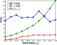
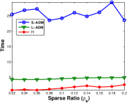
(a)	(b)

Figure 2: Performance of the standard ADM (S-ADM for short), LTSVD ADM (L-ADM for short) and $l_{1}$ filtering under different rank ratios $\rho_{r}$ and sparsity ratios $\rho_{s}$, where the matrix size is $1000\times 1000$. The $x$-axis represents the rank ratio (a) or sparsity ratio (b). The $y$-axis represents the CPU time (in seconds).

4.1.2 $l_{1}$ Filtering vs. Factorization Method

We then compare the proposed $l_{1}$ filtering with a factorization method (i.e., LMaFit) on solving (2). To test the ability of these algorithms in coping with corruptions with large magnitude, we multiply a scale $\mathbf{\sigma}$ to the sparse matrix, i.e., $\mathbf{M}=\mathbf{L}_{0}+\sigma\mathbf{S}_{0}$. We fix other parameters of the data ($m=1000$, $r=0.01m$ and $\rho_{s}=0.01$) and vary the scale parameter $\sigma$ from 1 to 10 to increase the magnitude of the sparse errors.

The computational comparisons are presented in Figure 3. Besides the CPU time and relative error, we also measure the quality of the recovered $\mathbf{L}^{*}$ by its maximum difference (MaxDif) and average difference (AveDif) to the true low-rank matrix $\mathbf{L}_{0}$, which are respectively defined as $\mbox{MaxDif}=\max(|\mathbf{L}^{*}-\mathbf{L}_{0}|)$ and $\mbox{AveDif}=(\sum_{ij}|\mathbf{L}^{*}-\mathbf{L}_{0}|)/m^{2}$. One can see that the performance of LMaFit dramatically decreases when $\sigma\geq 3$. This experiment suggests that the factorization method fails when the sparse matrix dominates the low-rank one in magnitude. This is because a sparse matrix with large magnitudes makes rank estimation difficult or impossible for LMaFit. Without a correct rank, the low-rank matrix cannot be recovered exactly. In comparison, our $l_{1}$ filtering always performs well on the test data.

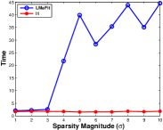
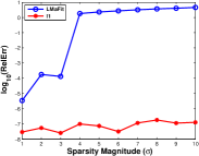
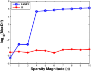
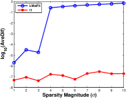
(a)	(b)	(c)	(d)

Figure 3: Performance of LMaFit and $l_{1}$ filtering under different sparsity magnitudes ($\sigma\in[1,10]$). The $x$-axes represent the sparsity magnitudes and the $y$-axes represent the CPU time (in seconds) (a), “RelErr” (b), “MaxDif” (c) and “AveDif” (d) in log scale, respectively.

In the following, we consider the problem of recovering deterministic low-rank matrix from corruptions. We generate an $m\times m$ “checkerboard” image (see Figure 4), whose rank is 2, and corrupt it by adding 10$\%$ impulsive noise to it. The corruptions (nonzero entries of the sparse matrix) are sampled uniformly at random. The image size $m$ ranges from 1000 to 5000 with an increment 500.

The results for this test are shown in Figure 4, where the first image is the corrupted checkerboard image, the second image is recovered by LMaFit and the third by $l_{1}$ filtering. A more complete illustration for this test can be seen from Figure 4(d), where the CPU time corresponding to all tested data matrix sizes are plotted. It can be seen that the images recovered by LMaFit and $l_{1}$ filtering are visually comparable in quality. The speeds of these two methods are very similar when the data size is small, while $l_{1}$ filtering runs much faster than LMaFit when the matrix size increases. This concludes that our approach has significant speed advantage over the factorization method on large scale data sets.

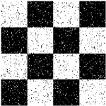
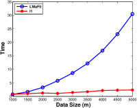
(a) Corrupted	(b) LMaFit	(c) $l_{1}$	(d) CPU Time

Figure 4: Recovery results for “checkerboard”. (a) is the image corrupted by 10$\%$ impulsive noise. (b) is the image recovered by LMaFit. (c) is the image recovered by $l_{1}$ filtering ($l_{1}$). (d) CPU time (in seconds) vs. data size ($m\in[1000,5000]$).

4.1.3 $l_{1}$ Filtering vs. Compressed Optimization

Now we compare $l_{1}$ filtering with a compressed optimization method (i.e., random projection). This experiment is to study the performance of these two methods with respect to the rank of the matrix and the data size. The parameters of the test matrices are set as follows: $\rho_{s}=0.01$, $\rho_{r}$ varying from 0.05 to 0.15 with fixed $m=1000$, and $m$ varying from 1000 to 5000 with fixed $\rho_{r}=0.05$. For the dimension of the projection matrix (i.e., $p$), we set it as $p=2r$ for all the experiments.

As shown in Figure 5, in all cases the speed and the numerical accuracy of $l_{1}$ filtering are always much higher than those of random projection.

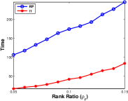
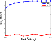
(a)	(b)
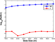
(c)	(d)

Figure 5: Performance of random projection (RP for short) and $l_{1}$ filtering. (a)-(b) are the comparison under different rank ratios ($\rho_{r}\in[0.05,0.15]$). (c)-(d) are the comparison under different data sizes ($m\in[1000,5000]$). In (a) and (c), the $y$-axes are the CPU times (in seconds). In (b) and (d), the $y$-axes are the relative errors in log scale.

4.2 Structure from Motion

In this subsection, we apply $l_{1}$ filtering to a real world vision application, namely structure from motion (SfM). The problem of SfM is to automatically recover the 3D structure of an object from a sequence of images of the object. Suppose that the object is rigid, there are $F$ frames and $P$ tracked feature points (i.e., $\mathbf{L}_{0}=\begin{bmatrix}\mathbf{X}\\ \mathbf{Y}\end{bmatrix}_{2F\times P}$), and the camera intrinsic parameters do not change. As shown in (Rao et al (2010)), the trajectories of feature points from a single rigid motion of the camera all lie in a liner subspace of $\mathbb{R}^{2F}$, whose dimension is at most four (i.e., $\mbox{rank}(\mathbf{L}_{0})\leq 4$). It has been shown that $\mathbf{L}_{0}$ can be factorized as $\mathbf{L}_{0}=\mathbf{A}\mathbf{B}$, where $\mathbf{A}\in\mathbb{R}^{2F\times 4}$ recovers the rotations and translations while the first three rows of $\mathbf{B}\in\mathbb{R}^{4\times P}$ encode the relative 3D positions for each feature point in the reconstructed object. However, when there exist errors (e.g., occlusion, missing data or outliers) the feature matrix is no longer of rank 4. Then recovering the full 3D structure of the object can be posed as a low-rank matrix recovery problem.

For this experiment, we first generate the 2D feature points $\mathbf{L}_{0}$ by applying an affine camera model (with rotation angles between 0 and $2\pi$, with a step size $\pi/1000$, and uniformly randomly generated translations) to the 3D “wolf” object , which contains $4344$ 3D points. Then we add impulsive noises $\mathbf{S}_{0}$ (the locations of the nonzero entries are uniformly sampled at random) to part (e.g., $5\%$ or $10\%$) of the feature points (see Figure 6). In this way, we obtain corrupted observations $\mathbf{M}=\mathbf{L}_{0}+\mathbf{S}_{0}$ with a size $4002\times 4344$.

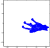
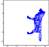
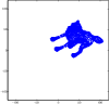
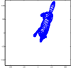
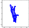
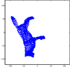
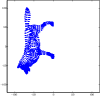
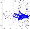
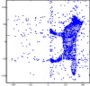
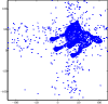
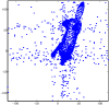
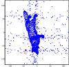
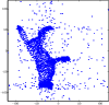
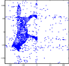
Figure 6: The illustrations of some trajectories (2D image frames) generated by the 3D “wolf” object (300th, 500th, $\cdots$, 1300th, 1500th frames). Top row: the ground truth trajectories. Bottom row: $10\%$ corrupted trajectories.

We apply our $l_{1}$ filtering to remove outliers (i.e., $\mathbf{S}_{0}$) and compute the affine motion matrix $\mathbf{A}$ and the 3D coordinates $\mathbf{B}$ from the recovered features (i.e., $\mathbf{L}_{0}$). For comparison, we also include the results from the robust subspace learning (RSL) (De la Torre and Black (2003)) and standard PCP (i.e., S-ADM based PCP). In Figure 7, we show the original 3D object, SfM results based on noisy trajectories and trajectories recovered by RSL, standard PCP and $l_{1}$ filtering, respectively. It is easy to see that the 3D reconstruction of RSL fails near the front legs and tail. In contrast, the standard PCP and $l_{1}$ filtering provide results with almost the same quality. Table 2 further compares the numerical behaviors of these methods. We measure the quantitative performance for SfM by the well-known mean 2D reprojection error, which is denoted as “ReprojErr” and defined by the mean distance of the ground truth 2D feature points and their reprojections. We can see that the standard PCP provides the highest numerical accuracy while its time cost is extremely high (9 times slower than RSL and more than 100 times slower than $l_{1}$ filtering). Although the speed of RSL is faster than standard PCP, its numerical accuracy is the worst among these methods. In comparison, our $l_{1}$ filtering achieves almost the same numerical accuracy as standard PCP and is the fastest.

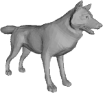
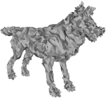
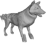
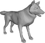
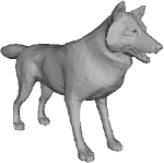
(a) Original	(b) Corrupted	(c) RSL	(d) S-PCP	(e) $l_{1}$-filtering

Figure 7: The SfM reconstruction. (a) is the original 3D object. (b)-(e) are SfM results using corrupted trajectory and the trajectories recovered by RSL, standard PCP (S-PCP for short) and $l_{1}$ filtering, respectively.

Table 2: Comparison among RSL, S-PCP and $l_{1}$ filtering on the structure from motion problem. We present CPU time (in seconds) and the numerical accuracy of tested algorithms. $\mathbf{L}_{0}$ and $\mathbf{S}_{0}$ are the ground truth and $\mathbf{L}^{*}$ and $\mathbf{S}^{*}$ are the solution computed by different methods.

Noisy Level	Method	RelErr	$\mbox{rank}(\mathbf{L}^{*})$	$\|\mathbf{S}^{*}\|_{l_{0}}$	Time	MaxDif($\mathbf{L}^{*}$)	AveDif($\mathbf{L}^{*}$)	ReprojErr
$5\%$	$\mbox{rank}(\mathbf{L}_{0})=4$,   $\|\mathbf{S}_{0}\|_{l_{0}}=869234$
	RSL	0.0323	4 (fixed)	15384229	93.05	32.1731	0.4777	0.9851
	S-PCP	$5.18\times 10^{-9}$	4	869200	848.09	$1.70\times 10^{-5}$	$2.47\times 10^{-8}$	$4.18\times 10^{-8}$
	$l_{1}$	$1.16\times 10^{-8}$	4	869644	6.46	$1.80\times 10^{-5}$	$3.61\times 10^{-7}$	$4.73\times 10^{-7}$
$10\%$	$\mbox{rank}(\mathbf{L}_{0})=4$,   $\|\mathbf{S}_{0}\|_{l_{0}}=1738469$
	RSL	0.0550	4 (fixed)	16383294	106.65	38.1621	0.9285	1.8979
	S-PCP	$6.30\times 10^{-9}$	4	1738410	991.40	$1.57\times 10^{-5}$	$4.09\times 10^{-8}$	$6.82\times 10^{-7}$
	$l_{1}$	$3.18\times 10^{-8}$	4	1739912	6.48	$5.61\times 10^{-5}$	$9.03\times 10^{-7}$	$1.26\times 10^{-6}$

4.3 Background Modeling

In this subsection, we consider the problem of background modeling from video surveillance. The background of a group of video surveillance frames are supposed to be exactly the same and the foreground on each frame is recognized as sparse errors. Thus this vision problem can be naturally formulated as recovering the low-rank matrix from its sum with sparse errors (Candés et al (2011)). We compare our $l_{1}$ filtering with the baseline median filter and other state-of-the-art robust approaches, such as RSL and S-PCP. When median filtering using all the frames, the complexity is actually also quadratic and the results are not good. So we only buffer 20 frames when using median filter to compute the background. For $l_{1}$ filtering, we set the size of the seed matrix as $20\times 20$.

For quantitative evaluation, we perform all the compared methods on the “laboratory” sequence from a public surveillance database (Benedek and Szirányi (2008)) which has ground truth foreground. Both the false negative rate (FNR) and the false positive rate (FPR) are calculated in the sense of foreground detection. FNR indicates the ability of the method to correctly recover the foreground while the FPR represents the power of a method on distinguishing the background. These two scores correspond to the Type I and Type II errors in the statistical test theory and are judged by the criterion that the smaller the better. One can see from Table 3 that RSL has the lowest FNR but the highest FPR among the compared methods. This reveals that RSL could not exactly distinguish the background. Although the speed of our $l_{1}$ filtering is slightly slower than median filtering on 20 frames, its performance is as good as S-PCP, which achieves the best results but with the highest time cost.

Table 3: Comparison among median filter (Median for short), RSL, S-PCP, and $l_{1}$ filtering on background modeling problem. “Resolution” and “No. Frames” denote the size of each frame and the number of frames in a video sequence, respectively. We present FNR, FPR and the CPU time (in seconds) for the “laboratory” data set. For our collected “meeting” data set, we only report the CPU time because there is no ground truth foreground for this video sequence.

Video	-	Median	RSL	S-PCP	$l_{1}$
“laboratory”	Resolution: $240\times 320$,  No. Frames: 887
	FNR	9.85	7.31	8.61	8.62
	FPR	9.18	10.83	8.72	8.76
	Time	42.90	3159.92	10897.96	48.99
“meeting”	Resolution: $576\times 720$,  No. Frames: 700
	Time	179.19	N.A.	N.A.	178.74

To further test the performance of $l_{1}$ filtering on large scale data set, we also collect a video sequence (named “meeting”) of 700 frames, each of which has a resolution $576\times 720$. So the data matrix is of size greater than $700\times 400000$, which cannot be fit into the memory of our PC. As a result, we cannot use the standard ADM to solve the corresponding PCP problem. As for RSL, we have found that it did not converge on this data. Thus we only compare the performance of median filter and $l_{1}$ filtering. The time cost is reported in Table 3 and the qualitative comparison is shown in Figure 8. We can see that $l_{1}$ filtering is as fast as median filtering with 20 frames, and median filter fails on this data set. This is because the mechanism of median filter is based on the (local) frame difference. Thus when the scene contains slowly moving objects (such as that in the “meeting” video sequence), median filter will not give good results. In contrast, the background and the foreground can be separated satisfactorily by $l_{1}$ filtering. This makes sense because our $l_{1}$ filtering can exactly recover the (global) low-rank structure for the background and remove the foreground as sparse errors.

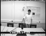
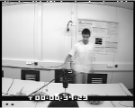
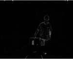
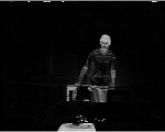
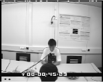
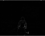
(a) Original	(b) Background (Median)	(c) Foreground (Median)	(d) Background ($l_{1}$)	(e) Foreground ($l_{1}$)

Figure 8: The partial background modeling results of median filter and $l_{1}$ filtering on the “meeting” video sequence. (b)-(c) and (d)-(e) are the the background ($\mathbf{L}^{*}$) and the foreground ($\mathbf{S}^{*}$) recovered by median filter and $l_{1}$ filtering, respectively.

5 Conclusion and Further Work

In this paper, we propose the first linear time algorithm, named the $l_{1}$ filtering method, for exactly solving very large PCP problems, whose ranks are supposed to be very small compared to the data size. It first recovers a seed matrix and then uses the seed matrix to filter some rows and columns of the data matrix. It avoids SVD on the original data matrix, and the $l_{1}$ filtering step can be done in full parallelism. As a result, the time cost of our $l_{1}$ filtering method is only linear with respect to the data size, making applications of RPCA to extremely large scale problems possible. The experiments on both synthetic and real world data demonstrate the high accuracy and efficiency of our method. It is possible that the proposed technique can be applied to other large scale nuclear norm minimization problems, e.g., matrix completion (Cai et al (2010)) and low-rank representation (Liu et al (2010)). This will be our future work.