Factorial Moments in Complex Systems

Laurent Schoeffel

CEA Saclay, Irfu/SPP, 91191 Gif/Yvette Cedex,

France

Factorial moments are convenient tools in particle physics to characterize the multiplicity distributions when phase-space resolution ($\Delta$) becomes small. They include all correlations within the system of particles and represent integral characteristics of any correlation between these particles. In this letter, we show a direct comparison between high energy physics and quantitative finance results. Both for physics and finance, we illustrate that correlations between particles lead to a broadening of the multiplicity distribution and to dynamical fluctuations when the resolution becomes small enough. From the generating function of factorial moments, we make a prediction on the gap probability for sequences of returns of positive or negative signs. The gap is defined as the number of consecutive positive returns after a negative return, thus this is a gap in negative return. Inversely for a gap in positive return. Then, the gap probability is shown to be exponentially suppressed within the gap size. We confirm this prediction with data.

1 Introduction

Multiplicity distributions and correlations between final-state particles in nuclear interactions are an important testing ground for analytic perturbative theory, as well as for Monte-Carlo (MC) models describing the hadronic final state [1]. Two-particle angular correlations have been extensively studied experimentally [2]. Specific statistical tools, namely the normalized factorial moments, have emerged in order to analyze in much details multiplicity distributions measured in restricted phase-space regions. The normalized factorial moments are defined as

$$F_{q}(\Delta)=\langle n(n-1)\ldots(n-q+1)\rangle/\langle n\rangle^{q},\qquad q=2,3,\ldots,$$

for a specified phase-space region of size $\Delta$. The number, $n$, of particles is measured inside $\Delta$ and angled brackets $\langle\ldots\rangle$ denote the average over all events. The factorial moments, along with cumulants [3] and bunching parameters [4], are convenient tools to characterize the multiplicity distributions when $\Delta$ becomes small. Indeed, for uncorrelated particle production within $\Delta$, Poisson statistics holds and $F_{q}=1$ for all $q$. Correlations between particles lead to a broadening of the multiplicity distribution and to dynamical fluctuations. In this case, the normalized factorial moments increase with decreasing $\Delta$. This effect is frequently called intermittency [5]. As a matter of fact, it has been noticed in [5] that the use of factorial moments allows to extract the dynamical signal from the Poisson noise in the analysis of the multiplicity signal in high energy reactions.

In addition, it has been shown that it is possible to define and compute a multi-fractal dimension, ${\cal D}_{q}$, for the theory of strong interactions [6, 7]

$$F_{q}(\Delta)=\langle n(n-1)\ldots(n-q+1)\rangle/\langle n\rangle^{q}\propto\Delta^{(q-1)(1-{\cal D}_{q}/d)}$$ (1)

where d is the dimension of the phase space under consideration ($d=2$ for the whole angular phase space, and $d=1$ if one has integrated over, say the azimuthal angle). In the constant coupling case ${\cal D}_{q}$ is well defined and reads

$${\cal D}_{q}=\gamma_{0}\frac{q+1}{q}$$ (2)

where $\gamma_{0}^{2}=4C_{A}{\alpha_{S}/2\pi}$, $\alpha_{S}$ is the strong interaction coupling constant, $C_{A}$ is the gluon color factor [6, 7]. The choice of the factorial moments as a specific tool in order to study the scaling behavior of the high energy multiplicity distributions is then useful to analyze the underlying dynamics of the processes. In principle, we can extend this last idea to other fields where factorial moments can be defined.

2 Generating Function for Factorial Moments

The multiplicity distribution is defined as $P_{n}={\sigma_{n}}/{\sum_{n=0}^{\infty}\sigma_{n}}$, where $\sigma_{n}$ is the cross section of an $n$-particle production process (the so-called topological cross section) and the sum is over all possible values of $n$ so that

$$\sum_{n=0}^{\infty}P_{n}=1.$$ (3)

The generating function can be defined as

$$G(z)=\sum_{n=0}^{\infty}P_{n}(1+z)^{n},$$ (4)

which substitutes an analytic function of $z$ in place of the set of numbers $P_{n}$. Then, we obtain the factorial moment or order $q$ as

$$F_{q}=\frac{1}{\langle n\rangle^{q}}\cdot\frac{d^{q}G(z)}{dz^{q}}\vline_{z=0},$$ (5)

and the corresponding definition for cumulants

$$K_{q}=\frac{1}{\langle n\rangle^{q}}\cdot\frac{d^{q}\ln G(z)}{dz^{q}}.\vline_{z=0},$$ (6)

The expression for $G(z)$ can then be re-written as

$$G(z)=\sum_{q=0}^{\infty}\frac{z^{q}}{q!}\langle n\rangle^{q}F_{q}\;\;\;\;(F_{0}=F_{1}=1),$$ (7)

$$\ln G(z)=\sum_{q=1}^{\infty}\frac{z^{q}}{q!}\langle n\rangle^{q}K_{q}\;\;\;\;(K_{1}=1).$$ (8)

The physical meaning of these moments has been discussed in the previous section. Another interpretation can be seen from the above definitions if they are presented in the form of integrals of correlation functions. Let the single symbol $y$ represent all kinematic variables needed to specify the position of each particle in the phase space volume $\Delta$ [8]. A sequence of inclusive $q$-particle differential cross sections $d^{q}\sigma/dy_{1}\ldots dy_{q}$ defines the factorial moments as

$$F_{q}\sim\frac{1}{\langle n\rangle^{q}}\int_{\Delta}dy_{1}\ldots\int_{\Delta}dy_{q}\frac{d^{q}\sigma}{dy_{1}\ldots dy_{q}}.$$ (9)

Therefore, factorial moments include all correlations within the system of particles under consideration. They represent integral characteristics of any correlation between the particles whereas cumulants of rank $q$ represent genuine $q$-particle correlations not reducible to the product of lower order correlations.

3 Experimental Applications

In Ref. [9], it has been shown that factorial moments can be applied conveniently to quantitative finance. Namely, if we divide price series $y(t)$ in consecutive time windows of lengths $\Delta$, we can define a set of events. In each window, we have a certain number of positive returns $n_{+}$, where $y(t)-y(t-1)>0$, and similarly of negative returns $n_{-}$. If the sequence of returns is purely uncorrelated, following a Gaussian statistics at all scales, we expect $F_{q}=1$ for all $q$.

As explained in previous sections, correlations between returns may lead to a broadening of the multiplicity distributions ($n_{+}$ or $n_{-}$ or even a combination of both) and to dynamical fluctuations. In this case, the factorial moments may increase with decreasing $\Delta$, or increasing the number of bins that divide $\Delta$. In Ref. [9], we have used the factorial moment of second order $F_{2}$ for like-sign returns

$$F_{2}^{++}=\frac{1}{N_{events}}\sum_{events}\frac{\sum_{k=1}^{n_{bins}}\left\{n_{k}^{+}(n_{k}^{+}-1)\right\}/n_{bins}}{(\langle n^{+}\rangle/n_{bins})^{2}}$$ (10)

where $\langle n\rangle$ is the average number of positive returns in the full time window ($\Delta$), $n_{bins}$ denotes the number of bins in this window and $n_{k}^{+}$ is the number of positive returns in $k$-th bin. Similarly, we have defined the unlike-sign returns for $F_{2}$

$$F_{2}^{+-}=\frac{1}{N_{events}}\sum_{events}\frac{\sum_{k=1}^{n_{bins}}\left\{n_{k}^{+}n_{k}^{-}\right\}/n_{bins}}{\langle n^{+}\rangle\langle n^{-}\rangle/(n_{bins})^{2}}$$ (11)

with similar notations. Considering different price series, we have shown that for a small resolution in time window [9], below $4$ to $8$ hours, a deviation with respect to pure Gaussian fluctuations is observed from the shape of second order factorial moments (10) and (11) [9]. Results are reminded in Fig. 1.

In order to compare the strength of the intermittency obtained in financial data, it is interesting to provide a comparison with standard high energy phenomenon in particle physics [8, 10]. In what follows we discuss the results obtained with two of the most widely used $e^{+}e^{-}$ MC event generators, JETSET [11] and HERWIG [12]. As it is done in the finance case, we define moments for like-charge and unlike-charge combinations of particles separately. Fig. 2 shows the behavior of $F_{2}^{++,+-}(n_{bins})$ at a centre-of-mass energy $91.5$ GeV [10]. Without entering into details, we observe the rise of both observables with $n_{bins}\equiv b$ as in Fig. 1.

By comparing Fig. 1 and Fig. 2, we notice also that the intermittency is weak in the financial data w.r.t. high energy data, which is a reasonable observation.

4 Gap Probability

We can use the formalism introduced in section 2 in order to derive some further statements. From Eq. (7), we get

$$G(-1)=p_{0}$$

which corresponds to the probability to have zero particle in a phase space $\Delta$ or to have zero positive (resp. negative) returns in a given time window (finance case). This defines a gap, either in rapidity for particles or in duration for positive (resp. negative) returns. Let us use Eq. (6) to express $G(-1)$ in another way using cumulants $K_{q}$

$$G(-1)=\exp(-K_{1}+K_{2}/2!+...)$$

When we can neglect correlations within a large time window [9], we have $K_{2}=0$ and we conclude

$$p_{0}\simeq\exp(-K_{1})=\exp(-<n_{+,-}>)=\exp(-\rho\Delta)$$ (12)

where $\Delta$ represents either the phase space or the time window. This last expression is very simple and instructive. It states that the gap probability is exponentially suppressed either in rapidity or in time. This is illustrated in Fig. 3 for the finance case. We observe the distribution of events (probability distribution) as a function of the size of the gap. The gap is defined as the number of consecutive positive returns after a negative return, thus this is a gap in negative return. Inversely for a gap in positive return. This gap is given in number of time units for the financial time series considered. In Fig. 3, we display results for the Euro future contract series over 10 years, sampled in two different time units. In both cases we observe effectively an exponential fall of the probability distribution as a function of the gap size. As illustrated also in Fig. 3, this exponential fall does not depend on the sampling. This confirms the prediction of Eq. (12). The case of particle physics is more complex, see Ref. [13].

5 Conclusion

In this letter, we have discussed a direct comparison between high energy physics and quantitative finance results on factorial moments analysis. Both for physics and finance, we have illustrated that correlations between particles lead to a broadening of the multiplicity distribution and to dynamical fluctuations when the resolution becomes small enough. From the generating function of factorial moments, we have shown that $p_{0}\simeq\exp(-\rho\Delta)$. This expression states that the gap probability is exponentially suppressed within the gap size. The gap is defined as the number of consecutive positive returns after a negative return, thus this is a gap in negative return. Inversely for a gap in positive return. We have confirmed this prediction with data.

Figure 1: Euro future contract. Like-sign and unlike-sign factorial moments $F_{2}^{++}$ and $F_{2}^{+-}$ are displayed for $1$, $2$, $4$, $10$ or $20$ bins. The global time window of $16.5$ hours ($n_{bins}=1$). This provides a time resolution ranging from $1.6$ hours for $20$ bins till $16.5$ hours for $1$ bin. We observe that for $1$ and $2$ bins segmentation, $F_{2}^{++}$ is found equal to $1$ and $F_{2}^{++}$ is increasing above $1$ when the number of bins gets larger than $4$. This confirms that non-Gaussian fluctuations in the sequence of returns returns start to play a role when the resolution is below $4$ hours.

Figure 2: $e^{+}e^{-}$ collisions at high energy. Factorial moments $F_{2}(y,\varphi)$ for like-charge (a) and unlike-charge (b) factorial moments $F_{2}^{++}$ and $F_{2}^{+-}$, calculated using JETSET 7.4 for a center of mass energy of $91.5$ GeV. See text for details.

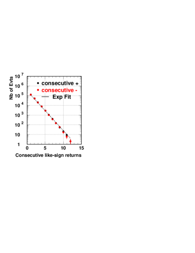
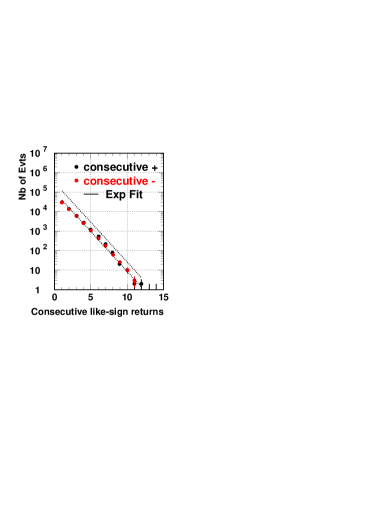
Figure 3: Left: Euro future contract sampled in 5min time units. Right: Euro future contract sampled in 30min time units. The distribution of events (probability distribution) is displayed as a function of the size of the gap. The gap is defined as the number of consecutive positive returns after a negative return, thus this is a gap in negative return. Inversely for a gap in positive return. The Euro future contract series over 10 years is sampled in two different time units (5min-Left and 30min-Right). In both cases, we observe effectively an exponential fall of the probability distribution as a function of the gap size. This confirms the relation derived in this letter $p_{0}\simeq\exp(-K_{1})=\exp(-<n_{+,-}>)=\exp(-\rho\Delta)$. We have presented an exponential fit on top of each plot. On the Right plot (30 minutes sampling), we super-impose also the fit obtained on the 5 minutes sampling, in order to show that the exponential slope is identical in both cases.

References

- [1] E.A. De Wolf, I.M. Dremin and W. Kittel, Phys. Rep. 270 (1996) 1.
- [2] ZEUS Collaboration, J. Breitweg et al., Eur. Phys. J C 12 (2000) 53.
- [3] A.H. Mueller, Phys. Rev. D 4 (1971) 150.
- [4] S.V. Chekanov and V.I. Kuvshinov, Acta Phys. Pol. B 25 (1994) 1189; S.V. Chekanov, W. Kittel and V.I. Kuvshinov, Z. Phys. C 74 (1997) 517.
- [5] A. Białas and R. Peschanski, Nucl. Phys. B 273 (1986) 703; Nucl. Phys. B 308 (1988) 857.
- [6] Y.L. Dokshitzer and I.M. Dremin Nuclear Physics B 402 (1993) 139.
- [7] W. Ochs and J. Wosiek, Phys. Lett. B289 (1992) 159, and Phys. Lett. B305 (1993) 144.
- [8] I. M. Dremin, V. Arena, G. Boca, G. Gianini, S. Malvezzi, M. Merlo, S. P. Ratti, C. Riccardi et al., Phys. Lett. B336 (1994) 119-124; I. M. Dremin, R. C. Hwa, Phys. Rev. D49 (1994) 5805-5811.
- [9] L. Schoeffel, arXiv:1108.5596.
- [10] J. Rames, arXiv:hep-ph/9411349.
- [11] T. Sjöstrand, CERN-TH.7112/93; H. U. Bengtsson and T. Sjöstrand, Comp. Phys. Comm. 46 (1987) 43.
- [12] G. Marchesini et al., Comp. Phys. Comm. 67 (1992) 465.
- [13] L. Schoeffel, Prog. Part. Nucl. Phys. 65 (2010) 9; Prog. Theor. Phys. Suppl. 187 (2011) 179.