Gluon mass through ghost synergy

Abstract

In this work we compute, at the “one-loop-dressed” level, the nonperturbative contribution of the ghost loops to the self-energy of the gluon propagator, in the Landau gauge. This is accomplished within the PT-BFM formalism, which guarantees the gauge-invariance of the emerging answer. In particular, the contribution of the ghost-loops is automatically transverse, by virtue of the QED-like Ward identities satisfied in this framework. Using as nonperturbative input the available lattice data for the ghost dressing function, we show that the ghost contributions have a rather sizable effect on the overall shape of the gluon propagator, both for $d=3,4$. Then, by exploiting a recently introduced dynamical equation for the effective gluon mass, whose solutions depend crucially on the characteristics of the gluon propagator at intermediate energies, we show that if the ghost loops are removed from the gluon propagator then the gluon mass vanishes. These findings strongly suggest that, at least at the level of the Schwinger-Dyson equations, the effects of gluons and ghosts are inextricably connected, and must be combined suitably in order to reproduce the results obtained in the recent lattice simulations.

I Introduction

Our understanding of the infrared (IR) properties of the fundamental Green’s functions of Yang-Mills theories has improved considerably in the last few years, due to a variety of parallel efforts in lattice simulations Cucchieri:2007md ; Cucchieri:2007rg ; Cucchieri:2009zt ; Cucchieri:2011ga ; Cucchieri:2011um ; Cucchieri:2003di ; Cucchieri:2010xr ; Bowman:2007du ; Bogolubsky:2007ud ; Bogolubsky:2009dc ; Oliveira:2008uf ; Oliveira:2009eh , Schwinger-Dyson equations (SDEs) Aguilar:2008xm ; Aguilar:2010zx ; Binosi:2009qm ; RodriguezQuintero:2011vw ; RodriguezQuintero:2010wy ; Boucaud:2010gr ; Boucaud:2008gn ; Boucaud:2008ji , functional methods Braun:2007bx ; Szczepaniak:2010fe , and algebraic techniques Dudal:2008sp ; Dudal:2010tf ; Dudal:2011gd ; Kondo:2011ab . The majority of the aforementioned studies have focused on the low-momentum behavior the gluon and ghost propagators, which can be directly or indirectly related to some of the most fundamental nonperturbative phenomena of QCD, such as quark confinement, dynamical mass generation, and chiral symmetry breaking.

It is by now well-established that, in the Landau gauge, the lattice yields a gluon propagator and a ghost dressing function that are finite in the IR (in $d=3,4$) Aguilar:2008xm ; Aguilar:2010zx ; Boucaud:2008ji . Evidently, these lattice results furnish strong support to the idea of dynamical gluon mass generation through the well-known Schwinger mechanism Jackiw:1973tr ; Cornwall:1973ts ; Eichten:1974et , as proposed by Cornwall and others Cornwall:1981zr ; Bernard:1981pg . On the other hand, these important lattice findings have motivated the critical revision of the original Gribov-Zwanziger confinement scenario, leading to the formulation of its “refined” version Dudal:2008sp . In addition, the “ghost-dominance” picture of QCD Alkofer:2000wg ; Fischer:2006ub , whose theoretical cornerstone has been the existence of a divergent (“IR-enhanced”) ghost dressing function, is at odds with the above lattice results, and, at least in this strict formulation, has been practically ruled out (in the Landau gauge, and for $d=3,4$) Aguilar:2008xm ; Aguilar:2010zx ; Boucaud:2008ji .

This last statement, however, does not necessarily mean that the ghost has been relegated to a marginal role in the QCD dynamics. In fact, compelling evidence to the contrary has emerged from detailed studies of the gap equation that controls the breaking of chiral symmetry and the dynamical generation of a constituent quark mass Fischer:2003rp ; Aguilar:2010cn . Specifically, the proper inclusion of the corresponding ghost sector (essentially the ghost dressing function and the quark-ghost kernel) is crucial for obtaining a realistic symmetry breaking pattern, with quark masses in the phenomenologically relevant range. The main lesson that can be drawn from the above studies is that even a finite (i.e., “non-enhanced”) ghost sector may have a strong numerical impact, at least in the framework of the SDEs, and affect nontrivially the realization of various underlying dynamical mechanisms Aguilar:2010cn . In fact, for the concrete case of the quark gap equation, the ghost contributions provide the necessary enhancement to the kernel of the gap equation precisely in the range of momenta around 1 GeV, which is the most relevant for obtaining the right type of quark mass solutions Roberts:1994dr .

Given the importance of the ghost sector for the dynamical generation of a constituent quark mass, it is natural to ask whether a similar situation applies in the case of the dynamical generation of an effective gluon mass. The main purpose of the present article is to address in detail this important question.

This problem is technically rather subtle, and hinges on the ability to treat self-consistently various field theoretic ingredients. To that end, we will employ the general formalism based on the pinch technique (PT) Cornwall:1981zr ; Cornwall:1989gv ; Binosi:2002ft ; Binosi:2003rr ; Binosi:2009qm and the background field method (BFM) Abbott:1980hw , which is particularly suited for dealing precisely with this type of problem. Specifically, the truncation scheme based on the PT-BFM formalism Aguilar:2006gr ; Binosi:2007pi ; Binosi:2008qk allows for subtraction of the ghost contributions to the gluon self-energy in a physically meaningful way (i.e., without introducing gauge artifacts). Indeed, in the conventional SDE formulation, any attempt to isolate the ghost contributions is bound to interfere with the transversality of the resulting gluon self-energy; this can be seen already at the one-loop level, where only the sum of the gluon and ghost diagrams (but not their individual contributions) is transverse. Instead, as was first pointed out in the classic paper by Abbott Abbott:1980hw , the calculation of the same diagrams using the BFM Feynman rules gives rise to two transverse contributions. This crucial property persists unaltered at the level of the SDE for the gluon self-energy: the SDE is composed by concrete subsets of “one-” and “two-loop dressed” diagrams, which are separately transverse, e.g., $q_{\mu}\Pi^{\mu\nu}_{c}(q)=0$, where $\Pi^{\mu\nu}_{c}(q)=(a_{3})^{\mu\nu}+(a_{4})^{\mu\nu}$ - see Fig. 1. Therefore, one can study the individual contribution of the different blocks [in this case $\Pi^{\mu\nu}_{c}(q)$] to the full gluon self-energy, without compromising the transversality of the answer (these points have been addressed in great detail in Aguilar:2006gr ; Binosi:2009qm ; Binosi:2007pi ; Binosi:2008qk )

Given that within the PT-BFM framework the ghost contributions to the gluon self-energy may be disentangled gauge invariantly, the next step will be to compute this particular contribution nonperturbatively, and then subtract it out from the full gluon propagator obtained from the lattice. The basic operating assumption underlying this analysis is that the gluon propagator found on the lattice coincides with that obtained from the solution of the full SDE series. Then, instead of solving the SDE series without the loops contained in $\Pi^{\mu\nu}_{c}(q)$ to determine the resulting gluon propagator (technically an impossible task at the moment), we compute nonperturbatively only the contribution of $\Pi^{\mu\nu}_{c}(q)$ and subtract it from the gluon propagator obtained from the lattice.

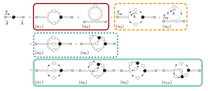
Figure 1: The SDE corresponding to the PT-BFM gluon self-energy $\Pi^{ab}_{\mu\nu}(q)$. The graphs inside each box form a gauge invariant subgroup, furnishing an individually transverse contribution. White (black) circles denote full propagators (vertices).

The nonperturbative computation of the aforementioned ghost contribution $\Pi^{\mu\nu}_{c}(q)$ [graphs $(a_{3})$ and $(a_{4})$ in Fig. 1] proceeds through the following main steps.

1. We introduce a suitable Ansatz for the full (background) gluon-ghost vertex, $\widetilde{\Gamma}_{\mu}$, [the black circle in graph $(a_{3})$] which satisfies automatically (i.e., by construction) the all-order Ward identity given in Eq. (6). This is an indispensable requirement for maintaining the gauge invariance (transversality) of the answer. The $\widetilde{\Gamma}_{\mu}$ obtained from this procedure [given in Eq.(18)] is expressed entirely in terms of the ghost propagator. As a result, the only quantity appearing finally inside the graphs $(a_{3})$ and $(a_{4})$ is the ghost propagator (or its dressing function).

2. We invoke the so-called “seagull identity”, given in Eq. (21), which enforces the cancellation of all sorts of seagull-type contributions, leading to the absence of quadratic divergences Aguilar:2009ke . Specifically, by means of this identity the purely seagull contribution of graph $(a_{4})$ cancels in its entirety against a term obtained from $(a_{3})$.

3. The remaining expression for $\Pi^{\mu\nu}_{c}(q)$ is renormalized subtractively, according to the rules of the momentum-subtraction (MOM) prescription.

4. The renormalized expression for $\Pi^{\mu\nu}_{c}(q)$ is then computed numerically, by substituting for the (infrared finite) ghost dressing function, appearing inside the integrals, the available lattice data for this quantity Cucchieri:2007md ; Cucchieri:2011um ; Bogolubsky:2007ud .

5. The latter contribution is subtracted from the entire gluon propagator obtained from the lattice, according to the formula given in Eq. (17).

The results turn out to be rather striking (see the right panels of Figs. 5, 8 and 11): the gluon propagator without $\Pi^{\mu\nu}_{c}(q)$ is significantly different from the full one. In addition, the results suggest a strong dependence on the space-time dimensionality: the effect of removing ghosts becomes considerably more enhanced as the space-time dimensionality is lowered.

At this point one can turn to the main question of this work, and study what would happen to the gluon mass if the ghost contributions, computed in the previous steps, were to be removed from the full gluon propagator obtained from the lattice. This question can be addressed in quantitative detail by means of the integral equation, derived recently in Aguilar:2011ux , which describes the evolution (i.e., momentum-dependence) of the dynamical gluon mass, $m^{2}(q^{2})$. This particular equation, given in Eq. (40), contains as its main ingredient the full gluon propagator  $\Delta$, which practically determines the form of its kernel. The detailed analysis of an approximate version of Eq. (40) carried out in Aguilar:2011ux reveals that the existence of physically acceptable solutions hinges crucially on the shape of the gluon propagator in the entire range of physical (Euclidean) momenta, and in particular on the precise behavior that $\Delta$ displays in the region between (1-5) $\rm GeV^{2}$. Specifically, in order for the gluon mass to be positive definite, the first derivative of the quantity $q^{2}\Delta(q^{2})$ (the “gluon dressing function”) must furnish a sufficiently negative contribution in the aforementioned range of momenta. Note that, as was shown in Aguilar:2011ux , the full $\Delta$ obtained from the lattice has indeed this particular property, giving rise [when inserted into Eq. (40)] to a dynamically generated gluon mass with the expected characteristics. Evidently, the main effect of removing the ghost contributions contained in $\Pi^{\mu\nu}_{c}(q)$ from $\Delta(q^{2})$ is to restrict significantly the negative area displayed by the (ghostless) $\Delta(q^{2})$ (see the right panels of Fig. 12), a fact which, in turn, leads to the vanishing of the gluon mass, i.e., the homogeneous Eq. (40) can only admit the trivial solution $m^{2}(q^{2})=0$.

Interestingly enough, this result appears to be completely analogous to what happens in the case of chiral symmetry breaking, where failure to include ghost contributions into the gap equation [the quark analogue of Eq. (40)] prevents the dynamical generation of a constituent quark mass Aguilar:2010cn . Thus, in the picture of QCD emerging from this analysis, ghosts and gluons must be in a state of harmonious synergy in order for a mass gap to be produced, regardless of the nature of the fundamental particle in question (gluon or quark).

The article is organized as follows. In Section II we study the general properties of the ghost sector in the Landau gauge and explain how it is possible within the PT-BFM framework to disentangle gauge-invariantly the (one-loop dressed) ghost contributions, $\Pi^{\mu\nu}_{c}(q)$, from the full gluon propagator. In Section III we derive the non-perturbative expression that determines $\Pi^{\mu\nu}_{c}(q)$ solely in terms of the ghost propagator and the coupling constant. In Section IV we evaluate numerically the expressions for $\Pi^{\mu\nu}_{c}(q)$ derived in the previous section, using as input the ghost dressing function obtained in recent lattice simulations Cucchieri:2007md ; Cucchieri:2011um ; Bogolubsky:2007ud . Next, we determine how the removal of $\Pi^{\mu\nu}_{c}(q)$ affects the overall shape of the resulting gluon propagator, for three different cases: $d=4$ and $N=2,3$, as well as $d=3$ and $N=2$, where $d$ is the dimensionality of space-time and $N$ is the number of colors [corresponding to the gauge group $SU(N)$]. In Section V we turn to the main question of the present work, and study in detail how the kernel of the dynamical integral equation governing the gluon mass gets modified after removing the aforementioned ghost contributions. Finally, our conclusions are presented in Section VI.

II Gauge invariant subtraction of ghost loops

In this section we first derive the formula that will determine the residual gluon propagator obtained from the full gluon propagator after removing from the latter the “one-loop dressed” ghost contributions, given by diagrams $(a_{3})$ and $(a_{4})$ in Fig. 1. Then, we work out the nonperturbative expression that determines the aforementioned ghost contribution in terms of integral involving the ghost dressing function.

The first important fact to recognize is the transversality of the ghost contributions to be removed. Specifically, denoting their sum by

$$\Pi_{c}^{\mu\nu}(q)=(a_{3})^{\mu\nu}+(a_{4})^{\mu\nu}\,,$$ (1)

we have that

$$(a_{3})_{\mu\nu} = -g^{2}C_{A}\int_{k}\!\widetilde{\Gamma}^{(0)}_{\mu}(k,q,-k-q)D(k)D(k+q)\widetilde{\Gamma}_{\nu}(k+q,-q,-k),$$

$$(a_{4})_{\mu\nu} = 2g^{2}C_{A}g_{\mu\nu}\int_{k}\!D(k).$$ (2)

In the equations above, $D^{ab}(q^{2})=\delta^{ab}D(q^{2})$ denotes the full ghost propagator, defined in terms of the ghost dressing function $F$ as

$$D(q^{2})=\frac{F(q^{2})}{q^{2}},$$ (3)

while $\widetilde{\Gamma}_{\mu}$ represents the three-particle vertex describing the interaction of the background gluon with a ghost and an antighost, with (all momenta entering)

$$i\Gamma_{c^{b}\widehat{A}^{a}_{\mu}\bar{c}^{c}}(r,q,p)=gf^{acb}\widetilde{\Gamma}_{\mu}(r,q,p);\qquad\widetilde{\Gamma}^{(0)}_{\mu}(r,q,p)=(r-p)_{\mu}.$$ (4)

Finally, $C_{A}$ is the Casimir eigenvalue of the adjoint representation [$C_{A}=N$ for $SU(N)$], and we have introduced the $d$-dimensional integral measure (in dimensional regularization) according to

$$\int_{k}\equiv\frac{\mu^{\epsilon}}{(2\pi)^{d}}\!\int\!\mathrm{d}^{d}k,$$ (5)

with $\mu$ the ’t Hooft mass, and $\epsilon=4-d$.

Then, by virtue of the PT-BFM Ward identity

$$iq^{\mu}\widetilde{\Gamma}_{\mu}(r,q,p)=D^{-1}(r)-D^{-1}(p),$$ (6)

it is immediate to establish the transversality of $\Pi_{c}^{\mu\nu}(q)$, namely Aguilar:2006gr

$$q_{\mu}\Pi_{c}^{\mu\nu}(q)=0.$$ (7)

Let us now denote by $\Pi^{\mu\nu}_{r}(q)$ the sum of the remaining subsets of diagrams in Fig. 1, i.e., both the gluon one- and two-loop dressed diagrams, as well as two-loop dressed ghost diagrams,

$$\Pi^{\mu\nu}_{r}(q)=\sum_{\begin{subarray}{c}i=1\\ i\neq 3,4\end{subarray}}^{10}(a_{i})^{\mu\nu}\,.$$ (8)

Again, due to the special Ward identities satisfied by the PT-BFM vertices, $\Pi^{\mu\nu}_{r}(q)$ is also transverse, and, of course, so is the full self-energy $\Pi^{\mu\nu}(q)$, given simply by

$$\Pi^{\mu\nu}(q)=\Pi^{\mu\nu}_{r}(q)+\Pi_{c}^{\mu\nu}(q).$$ (9)

The SDE for the full gluon propagator in the Landau gauge of the PT-BFM scheme assumes then the form

$$\Delta^{-1}(q^{2})P^{\mu\nu}(q)=\frac{q^{2}P^{\mu\nu}(q)+i\left[\Pi^{\mu\nu}_{r}(q)+\Pi^{\mu\nu}_{c}(q)\right]}{\left[1+G(q^{2})\right]^{2}},$$ (10)

where the gluon propagator $\Delta_{\mu\nu}(q)$ is defined as (we suppress color indices)

$$\Delta_{\mu\nu}(q)=-i\Delta(q^{2})P_{\mu\nu}(q);\qquad P_{\mu\nu}(q)=g_{\mu\nu}-\frac{q_{\mu}q_{\nu}}{q^{2}},$$ (11)

The function $G$ appearing in (10) is the form factor associated with $g_{\mu\nu}$ in the Lorentz decomposition of the auxiliary two-point function $\Lambda$, given by

$$\Lambda_{\mu\nu}(q) = -ig^{2}C_{A}\int_{k}\!\Delta_{\mu}^{\sigma}(k)D(q-k)H_{\nu\sigma}(-q,q-k,k)$$ (12)

$$= g_{\mu\nu}G(q^{2})+\frac{q_{\mu}q_{\nu}}{q^{2}}L(q^{2}).$$

This latter function, together with the auxiliary function $H$, are diagrammatically represented in Fig. 2; also notice that $H$ is related to the (conventional) gluon-ghost vertex by the identity

$$p^{\nu}H_{\nu\mu}(p,r,q)+\Gamma_{\mu}(r,q,p)=0,$$ (13)

and that, in the (background) Landau gauge, the following all order relation holds Grassi:2004yq ; Aguilar:2009pp

$$F^{-1}(q^{2})=1+G(q^{2})+L(q^{2}).$$ (14)

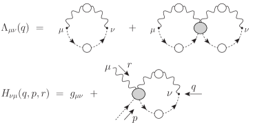
Figure 2: Definitions and conventions of the auxiliary functions $\Lambda$ and $H$. Gray blobs denote 1-PI kernels (with respect to vertical cuts).

Now, let us return to Eq. (10), and define in a completely analogous way the quantity $\Delta_{r}(q^{2})$, given by

$$\Delta_{r}^{-1}(q^{2})P^{\mu\nu}(q)=\frac{q^{2}P^{\mu\nu}(q)+i\Pi^{\mu\nu}_{r}(q)}{\left[1+G(q^{2})\right]^{2}}.$$ (15)

Evidently, $\Delta_{r}$ represents the propagator obtained by subtracting out (gauge invariantly) from the full propagator $\Delta$ the one-loop dressed ghost contributions. Then, taking the trace of both Eqs. (10) and (15), defining the trace of $\Pi^{\mu\nu}_{c}(q)$ as

$$\Pi_{c}(q^{2})\equiv\Pi^{\mu}_{c\,\mu}(q),$$ (16)

and solving for $\Delta_{r}$, we arrive at

$$\Delta_{r}(q^{2})=\Delta(q^{2})\left\{1-\frac{i\Delta(q^{2})\Pi_{c}(q^{2})}{(d-1)\left[1+G(q^{2})\right]^{2}}\right\}^{-1},$$ (17)

which represents our master formula.

In order to obtain the behavior of the propagator $\Delta_{r}(q^{2})$ from Eq. (17) we will (i) identify the full gluon propagator $\Delta(q^{2})$ with that obtained from the lattice, and (ii) determine nonperturbatively the quantity $\Pi_{c}$ from Eqs. (2) and (16), and evaluate it numerically using as input the lattice results for the ghost dressing function $F(q^{2})$. These points will be the subject of the next two sections.

III The nonperturbative expression for $\Pi_{c}(q^{2})$.

To accomplish step (ii) above, we first need to introduce an Ansatz for the fully-dressed ghost vertex $\widetilde{\Gamma}_{\mu}$, appearing in graph $a_{3}$ of Eq. (2), which satisfies the crucial Ward identity of Eq. (6) (this general procedure is known as the “gauge-technique Salam:1963sa ). The required Ansatz is easily constructed from that derived in Ball:1980ay for the case of scalar QED case, requiring the absence of kinematic or dynamical singularities. It reads

$$\widetilde{\Gamma}_{\mu}(r,q,p)=i\frac{(r-p)_{\mu}}{r^{2}-p^{2}}\left[D^{-1}(p^{2})-D^{-1}(r^{2})\right],$$ (18)

and evidently satisfies Eq. (6) when contracted with $q^{\mu}$. Obviously, the procedure of reconstructing the vertex by “solving” its Ward identity (known in general as “gauge technique”) leaves the transverse (automatically conserved) part of the vertex undetermined Salam:1963sa ; Kizilersu:2009kg . In this case this term has the form ${\cal A}(r,q)\left[(r\cdot q)p_{\mu}-(p\cdot q)r_{\mu}\right]$. This particular term vanishes as $q\to 0$, provided that the form factor ${\cal A}(r,q)$ does not diverge too strongly in that limit, which we will assume in what follows. Under this assumption, the transverse part of the vertex is subleading in the IR. On the other hand, its omission is known to affect the renormalization properties of the resulting SDE, a fact that forces one to renormalize subtractively instead of multiplicatively (see below).

Substituting (18) in the first equation of (2) and taking the trace, it is relatively straightforward to obtain the result

$$\Pi_{c}(q^{2})=g^{2}C_{A}\left[4T(q)-q^{2}R(q)\right],$$ (19)

where

$$R(q) = \int_{k}\!\frac{D(k+q)-D(k)}{(k+q)^{2}-k^{2}},$$

$$T(q) = \int_{k}\!k^{2}\frac{D(k+q)-D(k)}{(k+q)^{2}-k^{2}}+\frac{d}{2}\int_{k}\!D(k).$$ (20)

To further evaluate $\Pi_{c}(q^{2})$, we must invoke the so-called “seagull-identity” Aguilar:2009ke ,

$$\int_{k}\!k^{2}\frac{\partial{f}(k^{2})}{\partial k^{2}}+\frac{d}{2}\int_{k}\!f(k^{2})=0,$$ (21)

valid in dimensional regularization, which enforces the cancellations of all seagull-type of divergences. This identity guarantees the (nonperturbative) masslessness of the photon in scalar QED [by setting $f(k^{2})\to{\mathcal{D}}(k^{2})$, where ${\mathcal{D}}(k^{2})$ is the full massive scalar propagator], as well as the absence of quadratic divergences from the SDE determining the dynamical gluon mass [by equivalently setting $f(k^{2})\to\Delta(k^{2})$] Aguilar:2009ke .

For the case at hand, what we want to guarantee is that $\Pi_{c}(0)=0$; this must be indeed so, because the ghost-loop giving rise to $\Pi_{c}(q^{2})$ has no direct knowledge of the mass generating mechanism, namely the fact that $\Delta^{-1}(0)=m^{2}(0)$. The easiest way to appreciate this is by recalling that the mechanism responsible for endowing the gluon with a dynamical mass relies on the presence of massless poles in the nonperturbative tree-gluon [the black circle in graph $(a_{1})$ of Fig. 1], whereas the ghost vertex has the usual structure [note the absence of poles in the Ansatz of Eq. (18)] Aguilar:2011ux .

Evidently, in the limit $q\to 0$, the term $q^{2}R(q)$ vanishes, and so does $T(q)$, since

$$T(q)\ \stackrel{{\scriptstyle q\to 0}}{{\to}}\ T(0) = \int_{k}\!k^{2}\frac{\partial D(k^{2})}{\partial k^{2}}+\frac{d}{2}\int_{k}\!D(k),$$ (22)

$$= 0,$$

where in the last step we have employed Eq. (21), with $f(k^{2})\to D(k^{2})$.

In addition, note that the perturbative (one-loop) version of the terms $R(q)$ and $T(q)$, obtained from Eq. (20) by setting $D(k^{2})=1/k^{2}$, is given by

$$R^{(1)}(q) = -\int_{k}\,\frac{1}{k^{2}(k+q)^{2}},$$

$$T^{(1)}(q) = (d/2-1)\int_{k}\,\frac{1}{k^{2}}.$$ (23)

Evidently, due the dimensional regularization result $\int_{k}\!k^{-2}=0$ , we have that $T^{(1)}(q)=0$, and in the limit $q\to 0$, $q^{2}R^{(1)}(q)$ vanishes (in $d=3,4$).

It is clear that, when $d=4$, $R(q)$ is ultraviolet divergent, and must be properly renormalized, by introducing in the original Lagrangian the appropriate counterterm or wave-function renormalization (the need to renormalize is seen explicitly already at the level of $R^{(1)}(q)$, which diverges logarithmically). The (nonperturbative) renormalization of $\Pi_{c}(q^{2})$ that we will employ proceeds as follows. First of all, as happens almost exclusively at the level of SDEs, the renormalization must be carried out subtractively instead of multiplicatively. The main reason for that is the mishandling of overlapping divergences due to the ambiguity inherent in the gauge-technique construction of the vertex, related with the unspecified transverse part Curtis:1990zs .

The (subtractive) renormalization must be carried out at the level of (10). Specifically (setting directly $d=4$),

$$\Delta^{-1}(q^{2})=\frac{Z_{A}q^{2}+\frac{i}{3}\left[\Pi_{r}(q)+\Pi_{c}(q)\right]}{\left[1+G(q^{2})\right]^{2}},$$ (24)

where the renormalization constant $Z_{A}$ is fixed in the MOM scheme through the condition $\Delta^{-1}(\mu^{2})=\mu^{2}$. This condition, when applied at the level of Eq. (24), allows one to express $Z_{A}$ as

$$Z_{A}=[1+G(\mu^{2})]^{2}-\frac{i}{3\mu^{2}}\left[\Pi_{g}(\mu)+\Pi_{c}(\mu)\right].$$ (25)

Now, as is well-known Aguilar:2009nf ; Aguilar:2009pp , the validity of the BRST-driven relation (14) before and after renormalization prevents $G(\mu^{2})$ from vanishing when, according to the MOM prescription, $F(\mu^{2})=1$; instead, we must impose that $G(\mu^{2})=-L(\mu^{2})$. However, given that $L(x)$ is considerably smaller than $G(x)$ in the entire range of momenta, we can use the approximation $1+G(\mu^{2})\approx F^{-1}(\mu^{2})=1$, without introducing an appreciable numerical error. Thus, we obtain the following approximate equation for $Z_{A}$

$$Z_{A}=1-\frac{i}{3\mu^{2}}\left[\Pi_{r}(\mu)+\Pi_{c}(\mu)\right].$$ (26)

Finally, substituting Eq. (26) into Eq. (24), and defining (in a natural way) the renormalized $\Delta^{-1}_{r}(q^{2})$ as

$$\Delta^{-1}_{r}(q^{2})=\frac{q^{2}+\frac{i}{3}\left[\Pi_{r}(q)-(q^{2}/\mu^{2})\Pi_{r}(\mu)\right]}{[1+G(q^{2})]^{2}},$$ (27)

the renormalized version of the master formula (17) will read

$$\Delta_{r}^{-1}(q^{2})=\Delta^{-1}(q^{2})-\frac{i}{3}\frac{\left[\Pi_{c}(q)-(q^{2}/\mu^{2})\Pi_{c}(\mu)\right]}{[1+G(q^{2})]^{2}}.$$ (28)

Evidently (28) is obtained from (17) by replacing $\Delta^{-1}(q^{2})\to\Delta^{-1}_{R}(q^{2})$ (“$R$” for “renormalized”), and $\Pi_{c}(q)\to\Pi_{c,R}(q)$, where

$$\Pi_{c,R}(q)=\Pi_{c}(q)-(q^{2}/\mu^{2})\Pi_{c}(\mu).$$ (29)

As an elementary check, note that the application of the last formula at one loop yields

$$\Pi_{c,R}^{(1)}(q) = -g^{2}C_{A}q^{2}[R^{(1)}(q)-R^{(1)}(\mu)]$$ (30)

$$= \frac{ig^{2}C_{A}}{16\pi^{2}}q^{2}\ln\left(q^{2}/\mu^{2}\right),$$

which is the standard one-loop result of the PT-BFM Cornwall:1989gv ; Abbott:1980hw , renormalized in the MOM scheme.

For the ensuing numerical treatment of $R(q)$ and $T(q)$ carried out in the next section, it is advantageous to have the crucial property $T(0)=0$ a priori built in, in order to avoid possible deviations due to minor numerical instabilities. To that end, we introduce the quantity $\overline{T}$

$$\overline{T}(q) = T(q)-T(0)$$ (31)

$$= \int_{k}\!k^{2}\left[\frac{D(k+q)-D(k)}{(k+q)^{2}-k^{2}}-\frac{\partial D(k)}{\partial k^{2}}\right],$$

which has the property of ensuring (by construction) that $\overline{T}(0)=0$, while, at the same time, coinciding with the original $T$ for all momenta $q$.

In addition, it is convenient to re-express $R(q)$ and $\overline{T}(q)$ in terms of the ghost dressing function. Using Eq. (3), after some elementary algebra, one obtains

$$R(q) = -\int_{k}\frac{F(k)}{k^{2}(k+q)^{2}}+\int_{k}\!\frac{F(k+q)-F(k)}{k^{2}[(k+q)^{2}-k^{2}]},$$

$$\overline{T}(q) = \int_{k}\left[\frac{F(k+q)-F(k)}{(k+q)^{2}-k^{2}}-\frac{\partial F(k)}{\partial k^{2}}\right];$$ (32)

note that the angular integration of the first term in $R$ can be carried out analytically for any value of the space-time dimension $d$.

Finally, note that up until this point we have been working in Minkowski space. To make the transition to Euclidean space, we must employ the usual rules. Specifically, we set $\int_{k}\!=\mathrm{i}\!\int_{k_{\mathrm{{\scriptscriptstyle E}}}}$ and $q^{2}_{\mathrm{{\scriptscriptstyle E}}}=-q^{2}$, and use that

$$\Delta_{\mathrm{{\scriptscriptstyle E}}}(q^{2}_{\mathrm{{\scriptscriptstyle E}}})=-\Delta(-q^{2}_{\mathrm{{\scriptscriptstyle E}}});\qquad F_{\mathrm{{\scriptscriptstyle E}}}(q^{2}_{\mathrm{{\scriptscriptstyle E}}})=F(-q^{2}_{\mathrm{{\scriptscriptstyle E}}});\qquad G_{\mathrm{{\scriptscriptstyle E}}}(q^{2}_{\mathrm{{\scriptscriptstyle E}}})=G(-q^{2}_{\mathrm{{\scriptscriptstyle E}}}),$$ (33)

suppressing the subscript “E” in what follows.

IV Numerical evaluation of $\Pi_{c}(q^{2})$ and $\Delta_{r}(q^{2})$.

We will now proceed to perform the numerical analysis. Using the available lattice data on the ghost dressing function $F$, we evaluate the terms $R$ and $\overline{T}$ given in Eq. (32), and combine them following the Eqs. (19) and (29) to obtain the (renormalized) ghost contribution to the gluon self-energy $\Pi_{c}$ (of course, all relevant formulas must be properly “euclideanized”). Finally, we construct $\Delta_{r}$ using (17) and the lattice results available for the gluon propagator $\Delta$. This exercise is carried out for three different cases: $d=4$ and $N=2,3$, as well as $d=3$ and $N=2$.

IV.1 The case with $d=4$, $N=3$

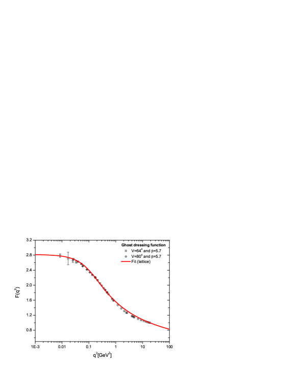
Figure 3: Left panel: Lattice result for the $SU(3)$ gluon propagator, $\Delta(q)$, in $d=4$, renormalized at $\mu=4.3$ GeV. The continuous line represents the fit given by Eq. (34). Right panel: The $SU(3)$ ghost dressing function, $F(q^{2})$, renormalized at the same point, $\mu=4.3$ GeV; the solid line corresponds to the fit given by Eq. (36).

In Fig. 3 we show the lattice results for the four-dimensional $SU(3)$ gluon propagator $\Delta(q^{2})$ (left panel), and the corresponding ghost dressing function $F(q^{2})$ (right panel), obtained from Bogolubsky:2007ud , and renormalized at $\mu=4.3$ GeV.

As has been discussed in detail in the literature Aguilar:2010cn ; Aguilar:2011ux ; Aguilar:2010gm , both sets of data can be accurately fitted in terms of IR-finite quantities. More specifically, for the case of $\Delta(q^{2})$, we have proposed a fit of the form Aguilar:2010gm

$$\Delta^{-1}(q^{2})=M^{2}(q^{2})+q^{2}\left[1+\frac{13C_{\rm A}g_{1}^{2}}{96\pi^{2}}\ln\left(\frac{q^{2}+\rho_{1}\,M^{2}(q^{2})}{\mu^{2}}\right)\right],$$ (34)

where

$$M^{2}(q^{2})=\frac{m_{0}^{4}}{q^{2}+\rho_{2}m_{0}^{2}}.$$ (35)

Notice that in the above expression, the finiteness of $\Delta^{-1}(q^{2})$ is assured by the presence of the function $M^{2}(q^{2})$, which forces the value of $\Delta^{-1}(0)=M^{2}(0)=m_{0}^{2}/\rho_{2}$. The continuous line on the left panel of Fig. 3 corresponds our best fit, which can be reproduced setting $m_{0}=520$ MeV, $g_{1}^{2}=5.68$, $\rho_{1}=8.55$ and $\rho_{2}=1.91$.

The $SU(3)$ lattice data for $F(q^{2})$, shown in the right panel of Fig. 3, will be fitted by the following expression

$$F^{-1}(q^{2})=1+\frac{9}{4}\frac{C_{\rm A}g_{1}^{2}}{48\pi^{2}}\ln\left(\frac{q^{2}+\rho_{3}M^{2}(q^{2})}{\mu^{2}}\right);\qquad M^{2}(q^{2})=\frac{m_{0}^{4}}{q^{2}+\rho_{2}m_{0}^{2}},$$ (36)

with the parameters given by $m_{0}=520$ MeV, $g_{2}^{2}=8.65$, $\rho_{2}=0.68$ and $\rho_{3}=0.25$ . Notice that the $M(q^{2})$ has the same power-law running as the one reported in Eq. (35) Lavelle:1991ve ; Aguilar:2007ie ; Oliveira:2010xc .

It is interesting to notice that the aforementioned fits share the following important properties: (i) they connect smoothly the IR and UV regions by means of a unique expression; (ii) their finiteness is associated with the presence of the parameter $M$ in the argument of the perturbative (renormalization group) logarithm, which it is responsible for taming the Landau pole and for doing the logarithm saturates at a finite value Aguilar:2010gm ; and (iii) for large values of $q^{2}$, Eqs. (34) and (36) reproduce their respective one-loop expressions in the Landau gauge.

The only missing ingredient for the actual nonperturbative determination of $\Pi_{c}$, and therefore $\Delta_{r}$, is the value of $\alpha_{s}=g^{2}/4\pi$. Instead of choosing a single value for $\alpha_{s}$, we will establish a certain physically motivated range of values, which will furnish a more representative picture of the numerical impact of the ghost corrections on the gluon propagator. The lower value for $\alpha_{s}$ will be fixed simply by resorting to the the 4-loop (perturbative) calculations in the MOM scheme Boucaud:2008gn , and extracting the value of $\alpha_{s}$ that corresponds to the subtraction point of $\mu=4.3$ GeV, used to renormalize the lattice data. The value so obtained is $\alpha_{s}=0.2$.

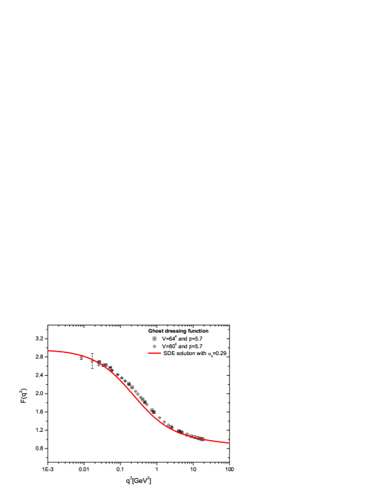
Figure 4: The solution of the SDE (37) that best matches the ghost dressing function data is obtained for $\alpha_{s}=0.29$.

In order to establish a reasonable upper bound, in a consistent way, we resort to the methodology employed in Aguilar:2009nf , which makes use of the standard SDE for the ghost dressing function, given by (Euclidean space)

$$F^{-1}(q^{2})=1+g^{2}C_{\rm{A}}\int_{k}\frac{1}{(k+q)^{2}}\left[1-\frac{(k\cdot q)^{2}}{k^{2}q^{2}}\right]\Delta(k)F(k+q),$$ (37)

derived in the Landau gauge, and under the assumption that the full ghost-gluon vertex is approximated by its tree-level value Aguilar:2009nf ; Cucchieri:2004sq . In this integral equation one substitutes for $\Delta(k)$ the fit given in Eq. (34), and solves it numerically for the unknown function $F(q^{2})$; evidently, for each value of $\alpha_{s}$ we obtain a different solution for $F(q^{2})$. The correct value of $\alpha_{s}$ is then determined as the one for which the corresponding (renormalized) solution best matches the lattice results (see Fig. 4); for $\mu=4.3$ GeV we obtain $\alpha_{s}=0.29$, showing that the perturbative MOM value ($\alpha_{s}=0.2$) is 30% lower.

The results obtained for the renormalized $R$ and $\overline{T}$, after substituting into the corresponding formulas our best fit for $F$, given by Eq. (36), are shown on the left panel of Fig. 5, together with the combination $q^{2}R-4\overline{T}$, which appears on the rhs of Eq. (19). It is clear that the contribution of the term $4\overline{T}$ is rather negligible; in a way this is to be expected, given that this term vanishes identically in perturbation theory (for all values of $q$), and vanishes nonperturbatively at the origin [viz. Eqs.(23) and (22), respectively].

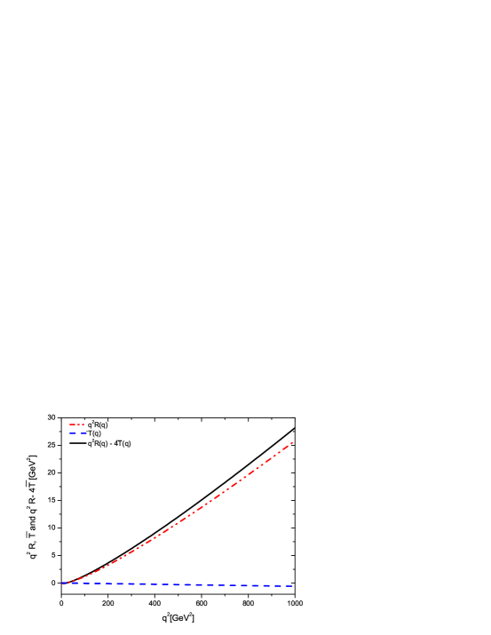
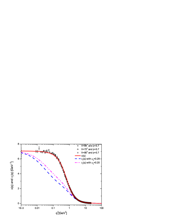
Figure 5: Left panel: Numerical evaluation of the ghost contribution $\Pi_{c}(q)$ to the gluon propagator using as input our best fit for the $d=4$, $N=3$ ghost dressing lattice data. Right panel: The removal of the one-loop dressed ghost contribution from the (lattice) gluon propagator results in a diminished “swelling” in the momentum region below 1 GeV².

Next, we use these results to construct $\Pi_{c}$, given in Eq. (29), and finally $\Delta_{r}$, expressed by Eq. (28) (Fig. 5 right panel), using both values of $\alpha_{s}$, namely $\alpha_{s}=0.29$ (SDE, red dotted line) and $\alpha_{s}=0.20$ (4-loop MOM, blue dashed-dotted line).

We then see that the net effect of removing the ghost contribution is to suppress significantly the support of the gluon propagator in the region below 1 GeV². Higher values of $\alpha_{s}$ increase the impact of the ghost contributions, but only slightly, as can be seen on the right panel of Fig. 5. As we will see in the next section, this “deflating” of the gluon propagator in the intermediate region of momenta, produced by the removal of the ghost contributions, has far-reaching consequences on the generation of a dynamical gluon mass.

IV.2 The case with $d=4$, $N=2$

It turns out that, changing the gauge group to $SU(2)$ does not significantly alter the characteristic qualitative behavior found in the $SU(3)$ case. Specifically, in Fig. 6 we show the gluon propagator (left panel), and the ghost dressing function (right panel), obtained from Cucchieri:2010xr and renormalized at $\mu=2.2$ GeV.

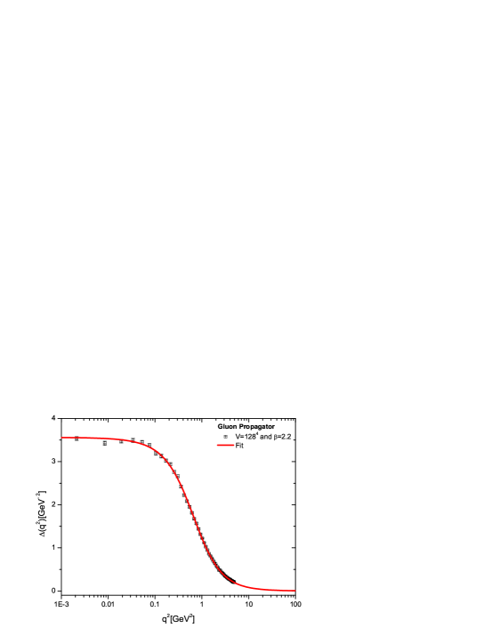
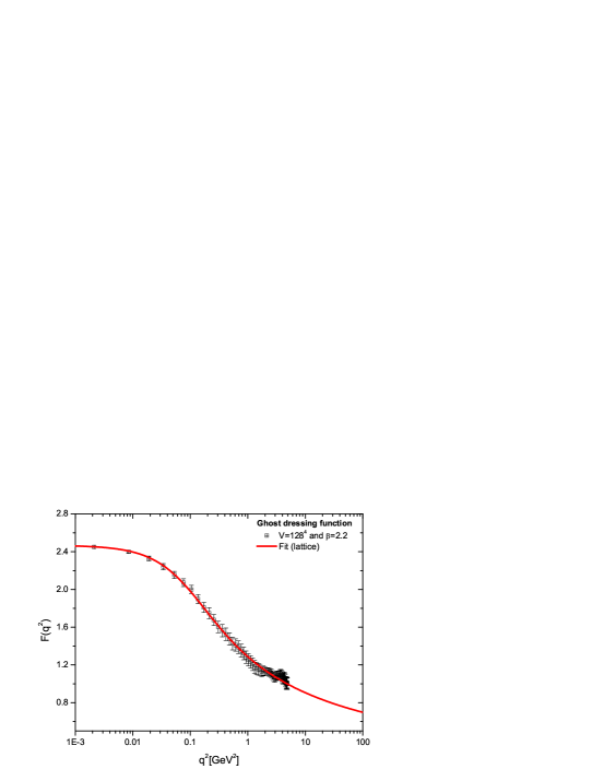
Figure 6: Left panel: Lattice results for the $SU(2)$ gluon propagator in $d=4$, renormalized at $\mu=2.2$ GeV. The continuous line represents our best fit to the data obtained from Eq. (34). Right panel: The $SU(2)$ ghost dressing function $F(q^{2})$, renormalized at the same point, $\mu=2.2$ GeV; the solid line corresponds to the best fit given by Eq. (36).

As in the $SU(3)$ case, the gluon and ghost data can be accurately fitted by the expressions (34) and (36), where now $C_{A}=2$ and the fitting parameters are $m_{0}=865$ MeV, $g_{1}^{2}=10.80$, $\rho_{1}=1.96$ and, $\rho_{2}=2.68$ (gluon) and $g_{2}^{2}=15.03$, $m_{0}=523\,$ MeV $\rho_{3}=0.215$ and $\rho_{4}=0.781$ (ghost).

The coupling $\alpha_{s}$ can be also fixed using the same procedure described in the previous subsection (Fig. 7); the value obtained from the SD solution that best matches the lattice data is in this case is $\alpha_{s}=0.99$.

Figure 7: The solution of the SDE (37) that best matches the ghost dressing function data is obtained for $\alpha_{s}=0.99$.

On the left panel of Fig. 8, we show the resulting curves for $R$ and $\overline{T}$ obtained through our best fit for $F$ given by Eq. (36). Then, using Eqs. (19) and (28) we combine the previous results to get the $SU(2)$ ghost self-energy $\Pi_{c}$ and, finally, $\Delta_{r}$ (right panel of the same figure). We use again two values for $\alpha_{s}$ namely the one obtained through the solution of the ghost SDE ($\alpha_{s}=0.99$) and a 30% lower one ($\alpha_{s}=0.70$). Evidently, the $SU(2)$ results do not differ qualitatively from those of the $SU(3)$ case: a lower value for $\alpha_{s}$ suppresses the ghost contribution to the gluon propagator, and the removal of the ghost gives rise to a lower curve in the region below 1 GeV².

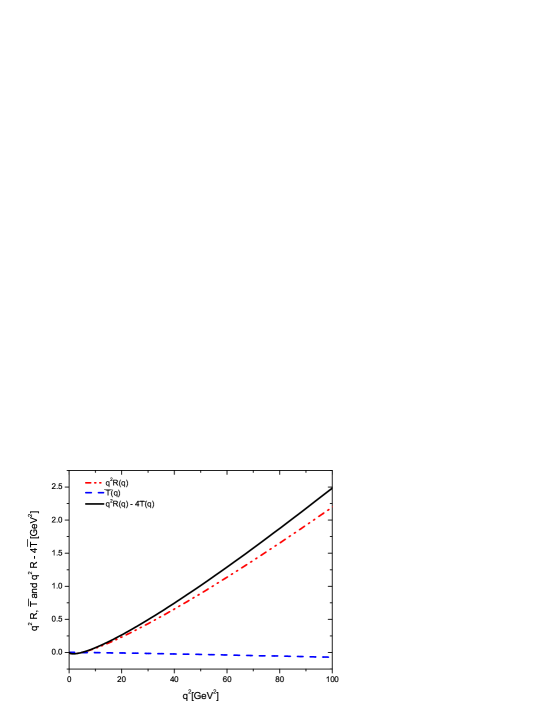
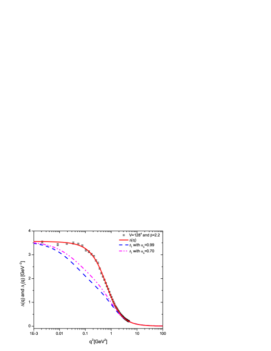
Figure 8: Left panel: Numerical evaluation of the ghost contribution $\Pi_{c}$ to the gluon propagator using as input our best fit (36) for the $d=4$, $N=2$ ghost dressing lattice data. Right panel: The removal of the one-loop dressed ghost contribution from the (lattice) gluon propagator causes, as in the $SU(3)$ case, a considerable suppression in the momentum region below 1 GeV².

IV.3 The case with $d=3$, $N=2$

Let us start, as in the previous cases, by showing in Fig. 9 the lattice results Cucchieri:2003di ; Cucchieri:2010xr for the three-dimensional gluon propagator $\Delta(q)$ (left panel) and the ghost dressing function $F(q)$ (right panel). Notice that, in Fig. 9, the lattice data for $\Delta(q)$ presented in Ref. Cucchieri:2003di ; Cucchieri:2010xr were appropriately rescaled, following the procedure explained in detail in Aguilar:2010zx , to match correctly the perturbative tail. Both $\Delta(q)$ and $F(q)$ saturate in the deep IR region, and can therefore be fitted by means of IR finite expressions.

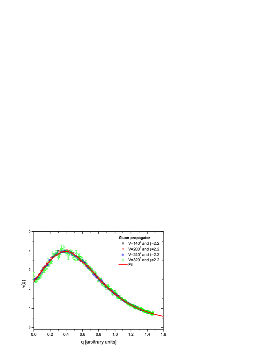
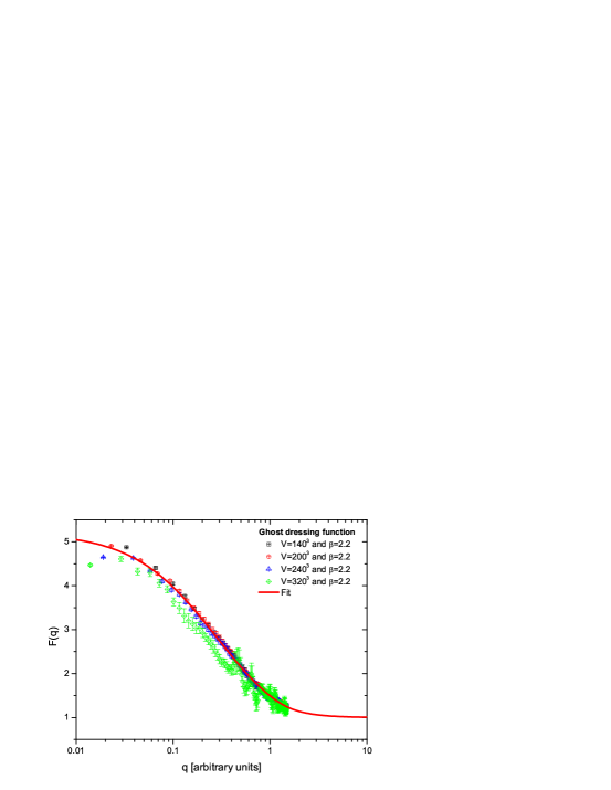
Figure 9: Left panel: Lattice results for the $SU(2)$ gluon propagator in $d=3$. The continuous line represents our best fit to the data obtained from Eq. (38). Right panel: Lattice data for the $SU$(2) ghost dressing function $F(q)$ in 3 dimensions; the solid line corresponds to the best fit given by Eq. (39).

In the case of the gluon propagator, an accurate fit is giving by

$$\Delta(q)=A\exp\left[-(q-q_{0})^{2}/w\right]+\frac{1}{a+bq+cq^{2}}\,,$$ (38)

where the fitting parameters are $A=0.49$, $q_{0}=0.11$, $w=0.37$, $a=0.43$, $b=-0.85$, and $c=1.143$. For the ghost dressing function, we use the following piecewise interpolator

$$F(q) = \frac{1}{a+bq+cq^{2}},\,\,\,\mbox{for}\quad q^{2}\leq 3$$ (39)

$$= 1+\frac{d}{eq+q^{2}},\,\,\,\mbox{for}\quad q^{2}>3$$

with fitting coefficients $a=0.19$, $b=0.61$, $c=-0.14$, $d=0.63$ and $e=0.26$ obtained by requiring the function to be continuous at $q^{2}=3$.

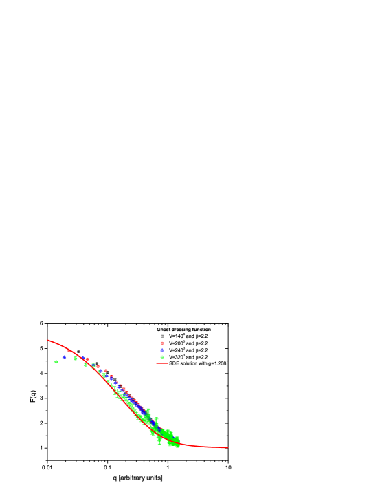
Figure 10: The solution of the SDE (37) that best matches the ghost dressing function data in $d=3$ is obtained for $g=1.208$.

The contribution of $R$ and $\overline{T}$ of Eq. (32) can be then evaluated using the above fit, and the results of this calculation are shown in the left panel of Fig. 11. Since $d=3$ Yang-Mills is a super-renormalizable theory, all aforementioned quantities are directly UV finite, and do not need to undergo renormalization.

The next step is to determine the value of the coupling constant $g$ (which, in $d=3$, has dimensions of $m^{1/2}$) entering in the formulas for $\Pi_{c}$ and $\Delta_{r}$, given by Eqs. (19) and (17), respectively. The procedure followed is the same as before, i.e. we will employ the three-dimensional ghost SDE, solve it for various values of $g$, and choose the one that best reproduces the lattice data for $F$. The most favorable case is shown in Fig. 10, where the solution for $F(q)$ obtained from the SDE with $g=1.208$ [in the same arbitrary mass units used in the plots of Fig. 9] (red line) is compared with the lattice results for the same quantity.

Next, substituting the results presented on the left panel of Fig. 11 into Eqs. (19) and (17), and using $g=1.208$, we compute $\Pi_{c}$ and $\Delta_{r}$. On the left panel of Fig. 11, we compare the residual propagator $\Delta_{r}$ (blue dashed line) with the full propagator $\Delta(q)$. Clearly, the effect in the tridimensional case is even more pronounced: the ghost contribution completely dominates over the rest, determining to a large extent the overall shape and structure of the propagator.

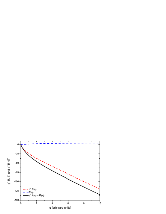
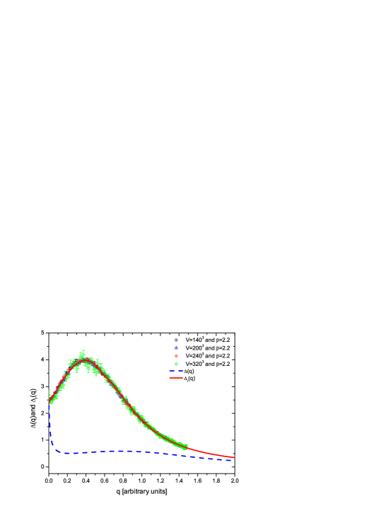
Figure 11: Left panel: Numerical evaluation of the ghost contribution $\Pi_{c}$ to the gluon propagator using as input our best fit for the $d=3$, $N=2$ ghost dressing lattice data. Right panel: The result of removing the one-loop dressed ghost contribution from the gluon propagator in $d=3$. The effect is much more dramatic than in the $d=4$ case, since all the structure is determined by the ghost contribution, while $\Delta_{r}$ has the sole (but crucial!) role of rendering the propagator finite at $q=0$.

V No gluon mass without ghost loops

In the previous section we have studied how the subtraction of the ghost contributions affects the profile of the gluon propagator. However, as we will now show, the effects goes way beyond a simple change in the overall propagator shape, modifying its salient qualitative characteristics, and in particular the generation of a dynamical gluon mass.

To establish this, we start from the dynamical equation describing the effective gluon mass, recently derived in Aguilar:2011ux ; it reads (Euclidean space)

$$m^{2}(q^{2})=\frac{2g^{2}C_{A}}{1+G(q^{2})}\int_{k}\!\left[k^{2}-\frac{(k\cdot q)^{2}}{q^{2}}\right]\frac{m^{2}(k+q)-m^{2}(k)}{(k+q)^{2}-k^{2}}\Delta(k)\Delta(k+q).$$ (40)

Taking the $q\to 0$ limit, one then gets

$$m^{2}(0) = \frac{2g^{2}C_{A}}{1+G(0)}\frac{d-1}{d}\int_{k}\!k^{2}[m^{2}(k)]^{\prime}\Delta^{2}(k)$$ (41)

$$= -\frac{4g^{2}C_{A}}{1+G(0)}\frac{d-1}{d}\int_{k}\!m^{2}(k)\Delta(k)\left[k^{2}\Delta(k)\right]^{\prime},$$

where in the last step we have used integration by parts. Introducing spherical coordinates (setting $y=k^{2}$) and the $d$-dimensional integral measure [notice that in (40) there is no dependence on the $d-2$ polar angles $\varphi_{i}$]

$$\int_{k}\ =\ \frac{1}{(2\pi)^{d}}\frac{\pi^{\frac{d-1}{2}}}{\Gamma\left(\frac{d-1}{2}\right)}\int_{0}^{\pi}\!{\rm d}\theta\sin^{d-2}\theta\int_{0}^{\infty}\!{\rm d}y\,y^{\frac{d}{2}-1},$$ (42)

Eq. (41) finally becomes

$$m^{2}(0)=-\frac{d-1}{d(4\pi)^{\frac{d}{2}}\Gamma\left(\frac{d}{2}\right)}\frac{4g^{2}C_{A}}{1+G(0)}\int_{0}^{\infty}\!{\rm d}y\,m^{2}(y){\cal K}_{d;N}(y),$$ (43)

with the kernel ${\cal K}_{d;N}$ given by

$${\cal K}_{d;N}(y)=y^{\frac{d}{2}-1}\Delta(y)[y\Delta(y)]^{\prime}.$$ (44)

The dependence of ${\cal K}_{d;N}$ on $N$ (the number of colors) is implicit in the form of $\Delta(y)$ that must be employed in each case, i.e., $\Delta(y)=\Delta_{N}(y)$. The same is true for $G(0)$ in (43), and, of course, $C_{A}=N$.

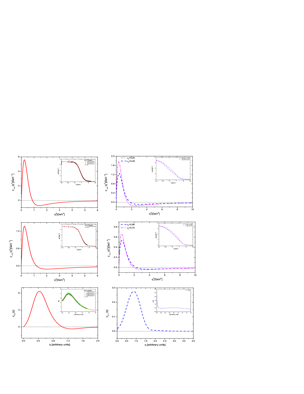
Figure 12: The kernel ${\cal K}_{d;N}$ of Eq. (44) constructed out of the lattice propagator $\Delta$ (left panels) and the ghost-less propagator $\Delta_{r}$ (right panels) for the $d=4$ $N=3$ (top row), $N=2$ (middle row) and $d=3$ $N=2$ (bottom row) cases. The insets show in each case the shape of the propagator used to evaluate the kernels.

Since the constant multiplying the integral is positive, the negative sign in front of Eq. (43) tells us that the required physical constraint $m^{2}(0)>0$ can be fulfilled if and only if the integral kernel ${\cal K}_{d;N}$ (constructed solely out of the gluon propagator) displays a sufficiently deep and extended negative region at intermediate momenta Aguilar:2011ux .

In the left panels of Fig. 12 we plot the kernels ${\cal K}_{d;N}$ obtained from the lattice data for the cases $d=4$, $N=3$ (top row) and $N=2$ (middle row), as well as $d=3$ $N=2$ (bottom row), considered in the previous section; they all posses the characteristic negative region that allows, at least in principle, the existence of solutions of Eq. (40), furnishing a positive value for the condition (41). We emphasize that, for the $d=4$ and $N=3,2$ cases such a solution has been explicitly found and studied in Aguilar:2011ux . Notice the striking resemblance between the kernels obtained for the different cases.

On the other hand, the situation changes substantially once the ghost loop is removed, in which case the kernels ${\cal K}_{d;N}$ must be constructed from $\Delta_{r}$ (right panels of the same figure). For $d=4$ one observes a shift towards higher $q$s of the zero crossing, and a correspondingly suppressed negative region; even though this is not sufficient to exclude per se the existence of a physical solution to the mass equation (40), a thorough study of the approximate equation derived in Aguilar:2011ux reveals that no physical solution may be found. The $d=3$ situation is even more obvious: the highly suppressed negative region present in this case cannot support solutions of (41) with $m^{2}(0)>0$, thus leaving as the only possibility the trivial $m^{2}=0$ solution.

The main conclusion one can draw, therefore, is that the ghosts play a fundamental role in the mechanism of dynamical gluon mass generation, since the failure to properly include them results in the inability of the theory to generate dynamically a mass for the gluon. This, in turn, implies that what is displayed in the right panels of Figs. 5, 8, 11, and 12 are not the gluon propagators one would actually obtain, assuming that one were actually able to perform this “experiment”, e.g., remove the ghosts on the lattice. Indeed, according to our results, if ghosts were not included, $m^{2}=0$, and thus $\Delta$ would not saturate in the IR at all!

To understand what happens, let us concentrate on the $d=4$, $N=3$ case and imagine a simplified setting, where one can switch off adiabatically the ghosts, neglecting all other effects this operation would entail (we will come back to this point at the end of this section). This could be achieved by multiplying the self-energy $\Pi_{c}$, appearing in Eq. (10), by a parameter $\gamma\in[0,1]$, such that when $\gamma=1$ the full $\Delta$ of the right panel of Fig. 5 is reproduced. Now, by slowly decreasing $\gamma$ (for fixed $\alpha$) one would give rise to a set of intermediate $\Delta_{r,\gamma}$ profiles, showing progressively less “swelling” in the $q^{2}<1$ [GeV²] region, and ideally one would get $\Delta_{r,0}\equiv\Delta_{r}$. However before that will happen, there will exist a critical value $\gamma_{c}$ for which the kernel ${\cal K}_{4;3}$ constructed from $\Delta_{r,\gamma_{c}}$ will fail to provide the required negative region that would ensure the positivity of $m^{2}(0)$, as calculated from the condition (43). At that point the theory will undergo a drastic change, showing a gluon propagator that does not saturate in the IR. Even though we cannot actually predict what such a propagator might behave like in the deep IR, it is likely that the typical singularity associated with the (perturbative) Landau pole (tamed by the presence of the mass) may reappear.

Obviously in this analysis we are neglecting any type of back-reaction due to the changes in the gluon propagator: to be sure, any modification to the latter quantity would affect not only the ghost – since the gluon propagator appears in fact in the ghost SDE, see Eq. (37) – but also the gluon mass, and therefore the IR saturation value – through Eqs. (40) and (41). While such effects might be numerically appreciable (changing, e.g., the critical value $\gamma_{c}$), we expect the qualitative description given above to persist.

VI Conclusions

In this article we have presented a detailed study of the impact of the ghost sector on the overall form of the gluon propagator in a pure Yang-Mills theory, for different space-time dimensions ($d=3,\ 4$) and $SU(N)$ gauge groups ($N=2,3$).

The key ingredients for performing this analysis have been basically two. To begin with, the PT-BFM framework allowed us to subtract out gauge-invariantly the “one-loop dressed” ghost diagrams from the SDE describing the full gluon propagator. Second, we have been able to express these ghost contributions as a simple integral involving the ghost dressing function only. This was achieved by employing a judicious Ansatz for the ghost-gluon vertex, obtained by solving the corresponding Ward identity, and by resorting to the “seagull-identity”, in order to enforce certain crucial properties. The nonperturbative evaluation of the resulting expressions have been carried out numerically, using available lattice data as input for the ghost dressing function. Our results reveal that the (“one-loop dressed”) ghost diagrams furnish a sizable contribution to the gluon propagator in $d=4$, and the dominant one in $d=3$.

The suppression of the gluon propagator induced by the removal of the ghost-loops has far-reaching consequences on the mechanism that endows gluons with a dynamical mass, associated with the observed IR-finiteness of the gluon propagator and the ghost-dressing function. Specifically, using a recently derived integral equation controlling the dynamics of the (momentum-dependent) gluon mass, we have demonstrated that when the reduced gluon propagators are used as inputs, the corresponding kernels are modified in such a way that no physical solutions may be found, thus failing to generate a mass gap for the pure Yang-Mills theory. Instead, as has been shown in Aguilar:2011ux , the use of the full gluon propagator in the same equation generates a physically acceptable gluon mass.

Once the results of the present work are combined with those of Aguilar:2010cn for the chiral symmetry breaking, a compelling picture of QCD emerges, where the generation of a dynamical mass for quarks and gluons requires the synergistic participation of all fields (physical and unphysical) of the theory.

- (1) A. Cucchieri and T. Mendes, PoS LAT2007, 297 (2007).
- (2) A. Cucchieri and T. Mendes, Phys. Rev. Lett. 100, 241601 (2008).
- (3) A. Cucchieri and T. Mendes, Phys. Rev. D 81, 016005 (2010).
- (4) A. Cucchieri and T. Mendes, PoS LATTICE2010, 280 (2010).
- (5) A. Cucchieri, T. Mendes, AIP Conf. Proc. 1343, 185-187 (2011).
- (6) A. Cucchieri, T. Mendes and A. R. Taurines, Phys. Rev. D 67, 091502 (2003).
- (7) A. Cucchieri and T. Mendes, PoS QCD-TNT09, 026 (2009)
- (8) P. O. Bowman et al., Phys. Rev. D 76, 094505 (2007).
- (9) I. L. Bogolubsky, E. M. Ilgenfritz, M. Muller-Preussker and A. Sternbeck, PoS LATTICE, 290 (2007).
- (10) I. L. Bogolubsky, E. M. Ilgenfritz, M. Muller-Preussker and A. Sternbeck, Phys. Lett. B 676, 69 (2009).
- (11) O. Oliveira, P. J. Silva, Phys. Rev. D79, 031501 (2009).
- (12) O. Oliveira and P. J. Silva, PoS LAT2009, 226 (2009).
- (13) A. C. Aguilar, D. Binosi and J. Papavassiliou, Phys. Rev. D 78, 025010 (2008).
- (14) A. C. Aguilar, D. Binosi and J. Papavassiliou, Phys. Rev. D 81, 125025 (2010).
- (15) D. Binosi and J. Papavassiliou, Phys. Rept. 479, 1-152 (2009).
- (16) J. Rodriguez-Quintero, Phys. Rev. D83, 097501 (2011).
- (17) J. Rodriguez-Quintero, JHEP 1101, 105 (2011).
- (18) Ph. Boucaud, M. E. Gomez, J. P. Leroy, A. Le Yaouanc, J. Micheli, O. Pene, J. Rodriguez-Quintero, Phys. Rev. D82, 054007 (2010).
- (19) Ph. Boucaud, F. De Soto, J. P. Leroy, A. Le Yaouanc, J. Micheli, O. Pene and J. Rodriguez-Quintero, Phys. Rev. D 79, 014508 (2009).
- (20) Ph. Boucaud, J. P. Leroy, A. L. Yaouanc, J. Micheli, O. Pene and J. Rodriguez-Quintero, JHEP 0806 (2008) 012.
- (21) J. Braun, H. Gies and J. M. Pawlowski, Phys. Lett. B 684, 262 (2010).
- (22) A. P. Szczepaniak and H. H. Matevosyan, Phys. Rev. D 81, 094007 (2010).
- (23) D. Dudal, J. A. Gracey, S. P. Sorella, N. Vandersickel and H. Verschelde, Phys. Rev. D 78, 065047 (2008).
- (24) D. Dudal, O. Oliveira, N. Vandersickel, Phys. Rev. D81, 074505 (2010).
- (25) D. Dudal, S. P. Sorella, N. Vandersickel, [arXiv:1105.3371 [hep-th]].
- (26) K. -I. Kondo, [arXiv:1103.3829 [hep-th]].
- (27) R. Jackiw, K. Johnson, Phys. Rev. D8, 2386-2398 (1973).
- (28) J. M. Cornwall, R. E. Norton, Phys. Rev. D8, 3338-3346 (1973).
- (29) E. Eichten, F. Feinberg, Phys. Rev. D10, 3254-3279 (1974).
- (30) J. M. Cornwall, Phys. Rev. D 26, 1453 (1982).
- (31) C. W. Bernard, Phys. Lett. B108, 431 (1982); Nucl. Phys. B219, 341 (1983).
- (32) R. Alkofer, L. von Smekal, Phys. Rept. 353, 281 (2001).
- (33) C. S. Fischer, J. Phys. G G32, R253-R291 (2006).
- (34) C. S. Fischer, R. Alkofer, Phys. Rev. D67, 094020 (2003).
- (35) A. C. Aguilar and J. Papavassiliou, Phys. Rev. D 83, 014013 (2011).
- (36) C. D. Roberts and A. G. Williams, Prog. Part. Nucl. Phys. 33, 477 (1994).
- (37) J. M. Cornwall and J. Papavassiliou, Phys. Rev. D 40, 3474 (1989).
- (38) D. Binosi and J. Papavassiliou, Phys. Rev. D 66(R), 111901 (2002).
- (39) D. Binosi and J. Papavassiliou, J. Phys. G 30, 203 (2004).
- (40) See, e.g., L. F. Abbott, Nucl. Phys. B 185, 189 (1981), and references therein.
- (41) A. C. Aguilar and J. Papavassiliou, JHEP 0612, 012 (2006).
- (42) D. Binosi and J. Papavassiliou, Phys. Rev. D 77(R), 061702 (2008).
- (43) D. Binosi and J. Papavassiliou, JHEP 0811, 063 (2008).
- (44) A. C. Aguilar and J. Papavassiliou, Phys. Rev. D 81, 034003 (2010).
- (45) A. C. Aguilar, D. Binosi and J. Papavassiliou, arXiv:1107.3968 [hep-ph].
- (46) P. A. Grassi, T. Hurth and A. Quadri, Phys. Rev. D 70, 105014 (2004).
- (47) A. C. Aguilar, D. Binosi and J. Papavassiliou, JHEP 0911, 066 (2009).
- (48) A. Salam, Phys. Rev. 130, 1287 (1963); A. Salam and R. Delbourgo, Phys. Rev. 135, B1398 (1964); R. Delbourgo and P. C. West, J. Phys. A 10, 1049 (1977); R. Delbourgo and P. C. West, Phys. Lett. B 72, 96 (1977).
- (49) J. S. Ball, T. -W. Chiu, Phys. Rev. D22, 2542 (1980).
- (50) A. Kizilersu and M. R. Pennington, Phys. Rev. D 79, 125020 (2009); A. Bashir, A. Kizilersu and M. R. Pennington, Phys. Rev. D 57, 1242 (1998).
- (51) D. C. Curtis and M. R. Pennington, Phys. Rev. D 42, 4165 (1990).
- (52) A. C. Aguilar, D. Binosi, J. Papavassiliou, JHEP 1007, 002 (2010).
- (53) M. Lavelle, Phys. Rev. D44, 26-28 (1991).
- (54) A. C. Aguilar, J. Papavassiliou, Eur. Phys. J. A35, 189-205 (2008).
- (55) O. Oliveira, P. Bicudo, J. Phys. G G38, 045003 (2011).
- (56) A. C. Aguilar, D. Binosi, J. Papavassiliou and J. Rodriguez-Quintero, Phys. Rev. D 80, 085018 (2009)
- (57) A. Cucchieri, T. Mendes and A. Mihara, JHEP 0412, 012 (2004).