Counting Low-Mass Stars in Integrated Light

Abstract

Low-mass stars ($M\lesssim 0.4M_{\odot}$) are thought to comprise the bulk of the stellar mass of galaxies but they constitute only of order a percent of the bolometric luminosity of an old stellar population. Directly estimating the number of low-mass stars from integrated flux measurements of old stellar systems is therefore possible but very challenging given the numerous variables that can affect the light at the percent level. Here we present a new population synthesis model created specifically for the purpose of measuring the low-mass initial mass function (IMF) down to $\sim 0.1M_{\odot}$ for metal-rich stellar populations with ages in the range $3-13.5$ Gyr. Our fiducial model is based on the synthesis of three separate isochrones and a combination of optical and near-IR empirical stellar libraries in order to produce integrated light spectra over the wavelength interval $0.35\mu m<\lambda<2.4\mu m$ at a resolving power of $R\approx 2000$. New synthetic stellar atmospheres and spectra have been computed in order to model the spectral variations due to changes in individual elemental abundances including C, N, Na, Mg, Si, Ca, Ti, Fe, and generic $\alpha$ elements. We demonstrate the power of combining blue spectral features with surface gravity-sensitive near-IR features in order to simultaneously constrain the low-mass IMF, stellar population age, metallicity, and abundance pattern from integrated light measurements. Finally, we show that the shape of the low-mass IMF can also be directly constrained by employing a suite of surface gravity-sensitive spectral features, each of which is most sensitive to a particular mass interval.

1. Introduction

In order to understand the formation and evolution of galaxies we must understand their stellar content. Attention is often directed at constraining the history of star formation, metallicity, and dust content of galaxies. In such work a key assumption is made: that the stellar initial mass function (IMF) is universal and equal to the IMF measured in the solar neighborhood. This assumption, and its influence on the derived physical properties of galaxies, is arguably the largest source of uncertainty in nearly all work related to the stellar populations of galaxies.

The IMF cannot be easily measured in extragalactic systems (or even in our own Galaxy) because the stellar luminosity-mass relation is steeper than the IMF — the former scales as $M^{3-4}$ on the main sequence (and is much steeper along the giant branches) while the latter scales as $M^{-2.3}$ or shallower in the solar neighborhood. Barring gross variation in these scalings in other galaxies, they imply that the light from any population of stars is dominated by the most massive stars that are still alive. The faint low-mass stars (i.e., $M<0.4M_{\odot}$), which probably dominate the total stellar mass budget in galaxies, contribute only of order $1$% to the integrated light.

In early type galaxies the problem is compounded by the fact that the stars that dominate the light, K and M giants, have a similar spectral type as the stars that dominate the mass budget, the K and M dwarfs. This implies that, to first order, the light from low mass stars looks similar to the light that dominates the flux. This is why it has historically been so difficult to measure the low-mass end of the IMF in early type galaxies.

Progress can be made by realizing that the spectra of M dwarfs and M giants at the same effective temperature display subtle but important differences. One of the first detections of such a difference was by Wing & Ford (1969) who discovered a very strong absorption feature at $0.99\mu m$ in the spectrum of an M dwarf that is not seen in M giants. This feature, now known as the Wing-Ford band, is attributed to absorption by FeH. It is very strong in late M dwarfs, but is absent in M giants. Among dwarfs, it is also very sensitive to effective temperature.

There are in fact a number of strong absorption features that vary with surface gravity at fixed effective temperature. These features include NaI at $0.82\mu m$, $1.14\mu m$ and $2.21\mu m$, CaI at $1.98\mu m$, CaII near $0.86\mu m$, CO near $2.30\mu m$, and H₂O lines that are numerous in the near-IR. The NaI, CaI and H₂O lines are strong in dwarfs and weak or absent in giants, while CaII and CO are strong in giants and weak in dwarfs (see e.g., Frogel et al., 1978; Kleinmann & Hall, 1986; Diaz et al., 1989; Ivanov et al., 2004; Rayner et al., 2009).

It was recognized early on that dwarf-sensitive and, to a lesser degree, giant-sensitive features could be used to count the number of low-mass stars in integrated light (e.g., Spinrad, 1962; Spinrad & Taylor, 1971; Cohen, 1978; Frogel et al., 1978, 1980; Faber & French, 1980; Carter et al., 1986; Hardy & Couture, 1988; Couture & Hardy, 1993; Vazdekis et al., 1996; Schiavon et al., 1997b, a, 2000; Cenarro et al., 2003). The fundamental difficulty then, as now, was the separation of abundance effects from giant-to-dwarf ratio effects. Both effects can change the strength of the gravity-sensitive lines. Since the average metallicity of massive elliptical galaxies is believed to be greater than our own Galaxy (e.g., Worthey et al., 1992; Trager et al., 2000; Thomas et al., 2005), the use of stellar spectra gathered in the solar neighborhood for the interpretation of metal-rich ellipticals was viewed with skepticism. The collection of M giant spectra in the Galactic bulge, which is more metal-rich than the disk, was recognized to be an important step in understanding the spectra of massive ellipticals (Carter et al., 1986; Frogel & Whitford, 1987), but this approach has not yet been as fruitful as initially hoped.

The early work on this topic suffered from additional uncertainties. The lack of accurate stellar evolution calculations across the main sequence and through advanced evolutionary phases implied that model construction suffered from major uncertainties that were difficult to quantify. Another major limitation was the poor near-IR detector technology that existed in the 1980s and 1990s. This made it very difficult to measure spectra at the sub-percent level precision necessary to measure the low-mass IMF in integrated light. In the intervening decades both of these uncertainties have been significantly reduced (though not eliminated). In addition, substantial progress has been made in understanding the response of stellar spectra to elemental abundance variations (e.g., Tripicco & Bell, 1995; Korn et al., 2005; Serven et al., 2005). All of these factors imply that the time is ripe to reconsider the possibility of measuring the IMF from integrated light spectra.

Recently we obtained spectra for eight massive galaxies in the Coma and Virgo clusters with $\sigma>250\ {\rm km\,s}^{-1}$ (van Dokkum & Conroy, 2010). Thanks both to the new CCDs installed on the Low Resolution and Imaging Spectrometer (LRIS) mounted on the Keck I telescope, and the stacking of these spectra in the restframe (thereby averaging out any residual sky emission and absorption problems), we were able to obtain accurate spectra at the $<0.5$% level. We combined these data with a preliminary version of the population synthesis model described herein to conclude that in these massive ellipticals the ratio of low to solar mass stars is much larger than in the Galaxy. The IMF in these massive ellipticals appeared to be much more ‘bottom-heavy’ compared to the IMF in the Galaxy.

The primary uncertainty in that work was the importance of abundance effects; the empirical stars used in our model are of approximately solar metallicity, while the ellipticals have metallicities in excess of solar and are $\alpha$-enhanced (e.g., Worthey et al., 1992; Trager et al., 2000; Thomas et al., 2005). In a follow-up to our initial results, we obtained spectra for four globular clusters (GCs) in M31 that have iron abundances and abundance patterns (i.e., $\alpha-$enhancement; [$\alpha$/Fe]) comparable to the massive ellipticals (van Dokkum & Conroy, 2011). A direct comparison of the spectra of these two populations revealed significant differences only in the surface gravity-sensitive lines. This constituted a critical test of our interpretation of the elliptical data because the M31 GCs have low mass-to-light ratios (Strader et al., 2011), and so could not have bottom-heavy IMFs. We therefore concluded that the ellipticals contained proportionally many more low mass stars than the GCs, again consistent with a dwarf-rich IMF in the massive ellipticals.

In the present work we present detailed population synthesis models with the goal of extracting the low-mass contribution to the integrated flux. The models span a range in age, metallicity, abundance patterns, IMFs, and cover the wavelength range $0.35\mu m<\lambda<2.4\mu m$ at a resolving power of $R\approx 2000$. An important feature of our approach is the use of synthetic spectra to gauge the sensitivity of the spectrum to individual elemental abundance variations. Our principle goal is to show that it is possible to separate the effects of IMF, age, metallicity, and abundance pattern, through the consideration of a variety of spectral features across the optical and near-IR wavelength range. These models can be contrasted with models such as Bruzual & Charlot (2003), which model spectral energy distributions at solar abundance patterns, and models that consider the effect of age, metallicity, and abundance patterns on the Lick index system (e.g., Trager et al., 2000; Thomas et al., 2003b; Schiavon, 2007). The model presented herein is, to our knowledge, the first to consider the response of the entire optical and near-IR spectrum to variations in individual elemental abundance patterns.

In the following sections we describe the details of the model ($\S$2), provide a brief comparison to data ($\S$3), present our results ($\S$4), and discuss several implications and set our findings in a broader context ($\S$5). A summary of our main conclusions is also provided ($\S$6).

2. Model Construction

2.1. Overview

Our goal is to construct models for the integrated light spectrum of a population of stars as a function of population age, metallicity, abundance pattern, and IMF. Two ingredients are necessary to construct such models: stellar evolution calculations (i.e., isochrones), and stellar spectral libraries. The isochrones dictate which stars are to be included in the synthesis, depending on the age and metallicity of the stellar population. The isochrones also determine the stellar mass of each star, given the physical parameters of the star (effective temperature, $\ T_{\rm eff}$, and bolometric luminosity, $\ L_{\rm bol}$). With the appropriate list of stars for a given age and metallicity, and the stellar mass of each star, the integrated light single stellar population (SSP) spectrum can be simply constructed from the integral:

$$f(\lambda)=\int_{m_{l}}^{m_{u}(t)}s(\lambda,m)\,\phi(m)\,{\rm d}m,$$ (1)

where the integral over stellar masses, $m$, ranges from the hydrogen burning limit, $m_{l}$, to the most massive star still alive at time $t$, $m_{u}(t)$. Throughout this paper we adopt $m_{l}=0.08M_{\odot}$. In the above equation, $f$ is the integrated spectrum, $s$ is the spectrum of an individual star, and $\phi$ is the IMF. We will consider four IMFs in the present work: a Chabrier (2003) IMF, which is a fit to the IMF of stars in the disk of the Milky Way, a Salpeter IMF, which has a logarithmic slope of $x=2.3$ ($x\equiv-$dln$\phi$/dlnm), a ‘bottom-heavy’ IMF that has a logarithmic slope of $x=3$, and a ‘bottom-light’ IMF advocated by van Dokkum (2008). The bottom-light IMF has a similar shape to the Chabrier IMF except that the former rolls over at $\approx 2M_{\odot}$ while the latter rolls over at $\approx 0.1M_{\odot}$.

In the following sections we describe the isochrones, stellar libraries, and synthesis techniques used to create integrated spectra as a function of population age, metallicity, and IMF.

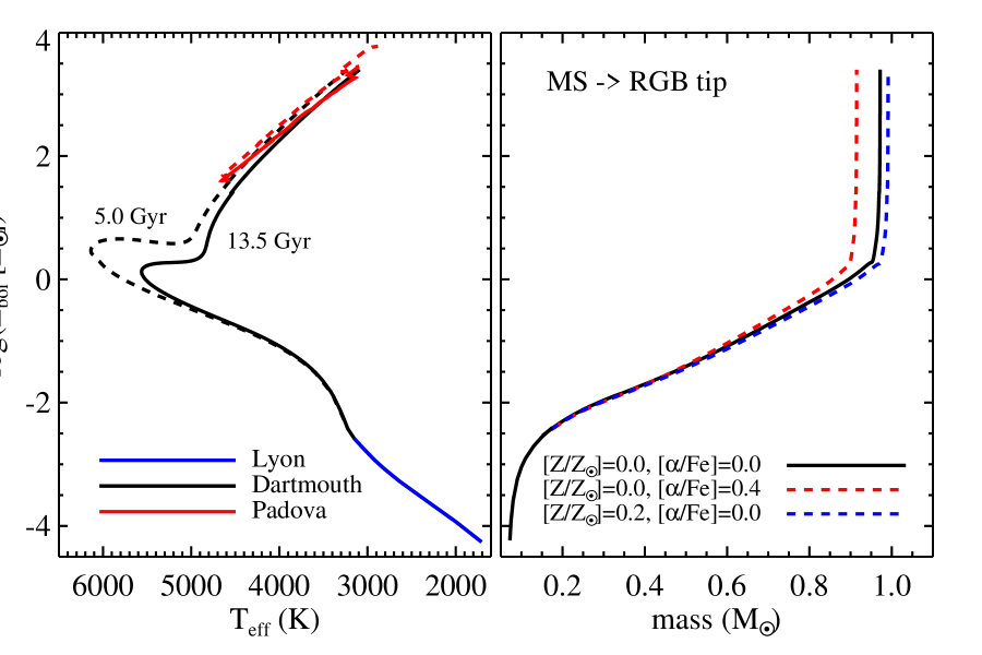
Figure 1.— Left panel: HR diagram showing how stellar evolution calculations from three groups are stitched together to create an isochrone that spans all stages of stellar evolution (through the end of the AGB) for all masses. Isochrones are shown for two ages as labeled in the panel. Right panel: Luminosity–mass relation as a function of metallicity. Here only the Dartmouth-based isochrones are shown for simplicity. Notice that the $L_{\rm bol}(M)$ relation is essentially insensitive to metallicity aside from the change in the turn-off mass.

2.2. Isochrones

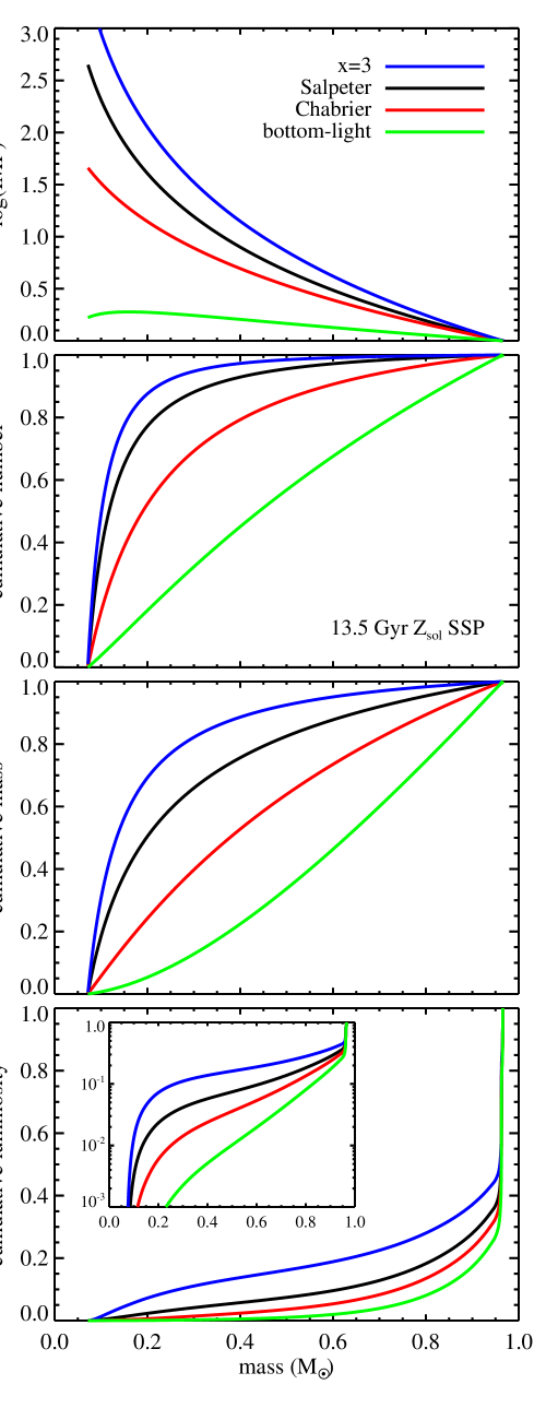
Figure 2.— Cumulative contribution to the total number of stars, total stellar mass, and bolometric luminosity as a function of stellar mass. Contributions are plotted as a fraction of the total. The inset in the bottom panel shows the cumulative luminosity on a logarithmic scale. Stellar remnants are not included in this figure. Results are shown for three IMFs, for models with an age of 13.5 Gyr and solar metallicity. The small contribution from low-mass stars to the integrated luminosity, despite their large contribution to the total number of stars and the stellar mass, is a direct consequence of the $L-M$ relation shown in Figure 1.

Accurate isochrones are required that extend from the hydrogen burning limit to the end of the asymptotic giant branch (AGB) phase. Unfortunately, no single set of publicly-available stellar evolution calculations exists that meets these requirements. We therefore need to stitch together several separate evolutionary calculations. For the bulk of the main sequence and red giant branch (RGB) we use the Dartmouth isochrones (Dotter et al., 2008), which have been shown to reproduce very well the main sequence morphology of old star clusters (An et al., 2009). These isochrones only extend to core helium ignition at the tip of the RGB. We therefore use the Padova isochrones (Marigo et al., 2008) for horizontal branch (HB) and AGB evolution. For $M<0.17M_{\odot}$ we use the Lyon isochrones (Chabrier & Baraffe, 1997; Baraffe et al., 1998). The maximum age in the Lyon models is 8 Gyr. Since these are low mass stars that evolve little over the range $3-14$ Gyr, we use their 8 Gyr models throughout. The precise value of 0.17$M_{\odot}$ was chosen so that the Dartmouth isochrones join smoothly with the Lyon isochrones in $\ T_{\rm eff}$ and $\ L_{\rm bol}$.

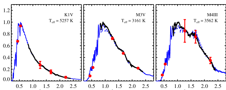
Figure 3.— Spectral energy distributions for three stars from the IRTF library. The IRTF spectra (solid black lines) are compared to optical and near-IR photometry (symbols) and our synthetic spectra (blue lines). The synthetic spectra were selected to have the same $\ T_{\rm eff}$ and ${\rm log}(g)$ as the observed stars and were scaled to match the observed spectra at the blue and red ends of the data. The theoretical spectra are dashed where they overlap in wavelength with the IRTF spectra, and solid where they are used to extrapolate the IRTF spectra. The SEDs were normalized to unity and smoothed by 100Å  for display purposes. Spectral types and estimated effective temperatures are shown in each panel.

The switch to the Lyon models below $0.17M_{\odot}$ is made because the Dartmouth models apply the surface boundary condition at the photosphere ($T=\ T_{\rm eff}$) rather than at the base of the atmosphere ($\tau=100$) as in the Lyon models. The depth at which the surface boundary condition is set is particularly important for the high density, low temperature environment encountered in very low mass stars. Stellar interior codes are not ideally suited to compute the physical conditions all the way to $T=\ T_{\rm eff}$. We note in passing that the Padova models are even less accurate at low masses than the Dartmouth models, and they only extend to $0.15M_{\odot}$, which is why we use the Padova models only for advanced evolutionary phases.

In the left panel of Figure 1 we show the resulting composite isochrone for a solar metallicity population with an age of 13.5 Gyr. For comparison, we also show an isochrone for a 5 Gyr solar metallicity population. The right panel of the same figure shows the $L-M$ relation for the main sequence and RGB. In this panel we also show the sensitivity of the $L-M$ relation to metallicity. The metallicity variations include a 0.2 dex increase in the total metal abundance (Z), and a 0.4 dex increase in the $\alpha$-elements ([$\alpha$/Fe]). Notice that while the main sequence turn-off mass changes slightly, the main sequence $L-M$ relation is almost entirely insensitive to these modest metallicity changes.

In the following we make use of the isochrones in two respects. First, they are used to determine which stars to include in the synthesis (e.g., stars that fall near the isochrone in the left panel of Figure 1). Second, they are used to assign masses to the stars based on $\ L_{\rm bol}$. Throughout this paper we will use the same solar metallicity isochrones, even when synthesizing models with different abundance patterns. This simplification is motivated by two facts: first, the $L-M$ relation is almost entirely insensitive to metallicity over the range of metallicities we will consider (right panel of Figure 1). This means that the masses assigned to stars are robust against changes in metallicity. Second, although changes in metallicity induce changes in the temperatures of stars, this effect is dwarfed by the much larger change in the spectra of stars at fixed temperature when metallicity varies, especially for old ages (¿5 Gyr; see Coelho et al., 2007; Schiavon, 2007; Lee et al., 2009).

In Figure 2 we show the IMFs considered herein and the cumulative contribution to the total number of stars, total stellar mass, and $\ L_{\rm bol}$ as a function of stellar mass and IMF. Stellar remnants are not included in the figure (though they are included in the total stellar mass budget in the rest of the paper). This figure summarizes the well-known fact that for standard IMFs low-mass stars dominate the total stellar mass and number of stars, but contribute only a small fraction of the total bolometric luminosity.

2.3. Empirical spectral libraries

Empirical spectral libraries constitute the core feature of our model. We make use of two separate libraries, the MILES library, which covers the wavelength range $0.35\mu m<\lambda<0.74\mu m$ (Sánchez-Blázquez et al., 2006), and the IRTF library of cool stars, which covers the wavelength range $0.81\mu m<\lambda<2.4\mu m$ (Cushing et al., 2005; Rayner et al., 2009).

We select stars from the main IRTF library that are not classified as chemically peculiar, have measured parallaxes (as obtained through SIMBAD) and that belong to luminosity class III or V. This leaves us with 91 stars ranging in spectral type from F0 to M9. The IRTF library includes flux calibrated spectra and $BVJHK$ photometry for each star. Absolute flux calibration is provided by the $JHK$ photometry. The spectral resolution is $R=2000$, and the signal-to-noise ratio varies from $\sim 100-1000$ with a median at $1\mu m$ of 700. We do not attempt to correct for dust extinction because the $E(B-V)$ values provided in the IRTF library are consistent with zero within the measurement uncertainties. In addition, the average distance to the stars in our sample is only 32 pc, suggesting that the spectra suffer from minimal extinction.

Effective temperatures are estimated for each IRTF star via the standard technique of using calibrated effective temperature - color relations. The $\ T_{\rm eff}-(V-K)$ relation for giants was adopted from Alonso et al. (1999) for F0-K5 giants, Ridgway et al. (1980) for K5-M6 giants, and from Perrin et al. (1998) for M6-M8 giants. For dwarfs we adopt the new $\ T_{\rm eff}$ scale from Casagrande et al. (2008, 2010). The $\ T_{\rm eff}$ scale of Casagrande et al. is consistent with earlier relations from Alonso et al. (1996) and Ramírez & Meléndez (2005), modulo $\sim 100$ K offsets that can be attributed to differences in the photometric absolute calibration adopted by different authors.

Bolometric luminosities were estimated for each IRTF star by extrapolating the observed spectrum both blueward and redward with a spectrum from our synthetic library (described in the next section) at the same $\ T_{\rm eff}$. Figure 3 illustrates this procedure. In each panel we show an IRTF spectrum, the accompanying $BVJHK$ photometry, and the synthetic spectrum used to extrapolate the IRTF spectrum both blueward and redward. Integrating over the full wavelength range then yields an estimate of $\ L_{\rm bol}$. The wide wavelength range of the IRTF spectra ensures that the bulk of the luminosity is directly measured for late-type stars. For example, the IRTF spectra samples $70-85$% of the bolometric luminosity for M-type stars, $40-70$% for G and K-type stars, and $20-40$% for F-type stars. The $B$ and $V$ photometry provide an important consistency check for our blueward extrapolation, as is evident from Figure 3.

For these reasons $\ L_{\rm bol}$ is a very robust parameter estimated for the IRTF stars. We therefore use $\ L_{\rm bol}$ to estimate the stellar mass for each IRTF star based on the $\ L_{\rm bol}-M$ relation shown in Figure 1 and described in $\S$2.2. The resulting mass—K-band luminosity relation for main sequence stars is shown in Figure 4. These isochrone-based masses are compared to the mass-luminosity relation derived for stars in binary orbits by Delfosse et al. (2000). The dynamicaly-estimated mass-luminosity relation is completely independent from our isochrone-based method, and so the impressive agreement provides strong support to our approach. Note that only two stars pin down the dynamically-based $M_{K}-M$ relation at $0.45M_{\odot}<M<0.6M_{\odot}$, so the mild divergence between the isochrone and dynamically-based masses in this range is not a significant source of concern. Once a mass is assigned to each star, we can then estimate its log$(g)$ based on the isochrones.

We have surveyed the literature for independently-derived physical parameters for our sample of 91 IRTF stars. We have found parameters for 35 of the stars (38% of the sample) in one or more of the MILES, ELODIE (Prugniel & Soubiran, 2001), SPOCS (Valenti & Fischer, 2005), and Indo-US (Valdes et al., 2004; Wu et al., 2011) libraries. The mean and standard deviation of the differences in $\ T_{\rm eff}$ are $\approx 20$ K and $\approx 100$ K, while for log($g$) the mean and standard deviation of the offsets are $\approx 0.05$ and $\approx 0.2$. These differences are comfortably within the typical errors on $\ T_{\rm eff}$ and log($g$) and give confidence to our independently-derived parameters. The differences are smallest between our parameters and those derived by the SPOCS survey, which is encouraging because the SPOCS survey consists of very high resolution ($R\sim 70,000$) spectra and very careful consideration of the available line data in their analysis. These surveys also provide estimates of the metallicity of each star. The average metallicity of the IRTF stars in common with MILES is $-0.07$, while for stars in common with SPOCS the average metallicity is $+0.05$. This supports our assumption that the IRTF stars are of approximately solar metallicity.

Figure 4.— Stellar mass–K-band absolute magnitude relation derived for the IRTF stars (symbols) compared to the relation derived from dynamically-based masses. Dynamical masses are derived from analysis of stars in binary orbits (Delfosse et al., 2000). IRTF stellar masses are derived from a theoretical $L_{\rm bol}(M)$ relation; see the text for details.

For two IRTF stars on the subgiant branch (HD10697 and HD25975) we have adopted the SPOCS and Indo-US values for their $\ T_{\rm eff}$ and log($g$) since those values are more accurate (being based on high resolution spectra), and result in better agreement with the location of 13.5 Gyr isochrones. Adoption of these parameters has essentially no impact on the resulting spectral synthesis, since the $\ T_{\rm eff}$ and log($g$) values are only used to pair IRTF and MILES stars.

The MILES library consists of $985$ stars covering a wide range in atmospheric parameters (Sánchez-Blázquez et al., 2006). The spectra have a FWHM of 2.5Å  and are relative flux calibrated, but not absolute flux calibrated. Atmospheric parameters ([Fe/H], log$(g)$, and $\ T_{\rm eff}$) were derived for MILES stars in Cenarro et al. (2007). We use the MILES library v9.1 (Falcón-Barroso et al., 2011), which corrects several small errors in previous releases. We removed hot variable stars and binaries (as identified in SIMBAD), and stars whose $\ T_{\rm eff}$ appeared to be in error based on visual inspection. This resulted in 28 stars being removed from the library.

The two coolest M dwarfs in the MILES library have spectral types M6 and M7. Both stars are magnetically active, as evidenced by strong Balmer emission lines in their optical spectra. Activity occurs in $\approx 60$% of such stars, and increases to $\approx 75$% for M8V stars (West et al., 2004). In addition to Balmer emission, these stars also display strong CaII H & K lines in emission. The third coolest M dwarf, of spectral type M3, also displays weak H & K emission lines. We will return to the importance of magnetic activity and associated chromospheric emission lines in cool M dwarfs later in the paper.

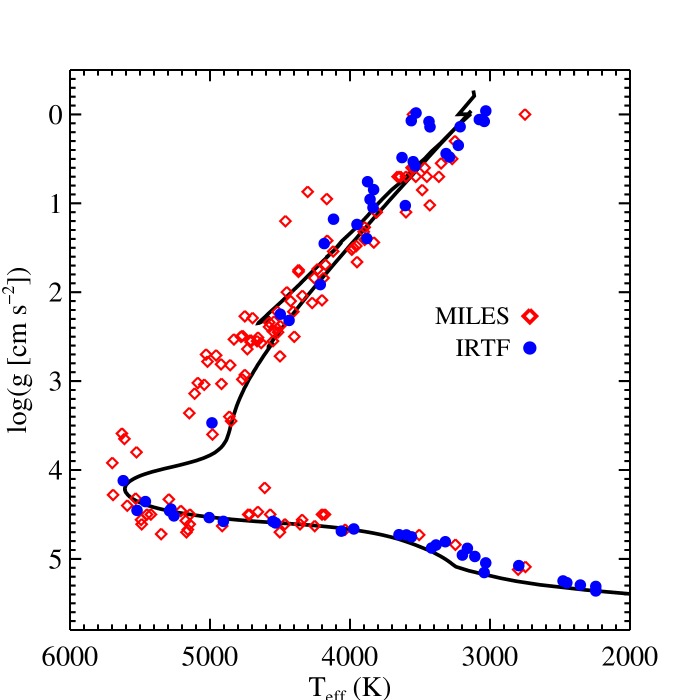
Figure 5.— Location in the HR diagram of stars from the empirical IRTF and MILES stellar libraries. Only the subset of IRTF stars used in our fiducial model are shown. Also shown is the fiducial isochrone ($Z=Z_{\sun}$, $t=13.5$ Gyr).

The MILES and IRTF libraries are combined in the following way. First, we select stars from MILES that have a metallicity of $-0.1<$[Fe/H]$<0.1$. This leaves 197 stars in the MILES library. We then take each IRTF star and pair it to the MILES library via interpolation in $\ T_{\rm eff}-{\rm log}(g)$ space. Figure 5 shows how MILES and IRTF stars populate this space. The MILES library is considerably larger than the IRTF library, so this pairing is straightforward. Once the pairing is made, the interpolated MILES spectrum is normalized against the $V-$band magnitude of the IRTF star. With this procedure we obtain an empirical spectrum for each star in $\ T_{\rm eff}-{\rm log}(g)$ space that spans the wavelength range $0.35\mu m<\lambda<2.4\mu m$ with only a modest gap at $0.74\mu m<\lambda<0.81\mu m$.

The astute reader will notice in Figure 5 that there are no MILES dwarf stars cooler than $\ T_{\rm eff}=2750$ K, corresponding to $M=0.15M_{\odot}$. Because of this, the five IRTF stars cooler than this are paired to the coolest MILES star available. As MILES spectra are always normalized to the $V-$band photometry of the IRTF stars, the overall change in $V-$band luminosity with mass is correctly modeled with our approach. It is only the surface gravity and temperature-sensitive lines that are affected by the lack of cooler dwarfs in the MILES library. Finally, we point out that $<0.15M_{\odot}$ stars contribute ten times less flux at $0.5\mu m$ compared to $>1\mu m$, so the approximate treatment of these stars in the optical should not be a source of concern.

2.4. Synthetic spectral libraries

Our empirical library, by construction, is very well suited for generating integrated light spectra of stellar populations with approximately Solar abundance ratios. However, it does not allow us to investigate changes in the overall metallicity or changes in the abundances of individual elements. We turn to synthetic spectra to incorporate this option in our modeling. These synthetic spectra are used to calculate relative changes with respect to a fiducial synthetic model, and these relative changes are then applied to indices that we measured from our empirical spectra (as in e.g., Trager et al., 2000; Thomas et al., 2003b; Schiavon, 2007). A synthetic spectral library does not exist that meets our needs, so we have generated our own library specifically for this project.

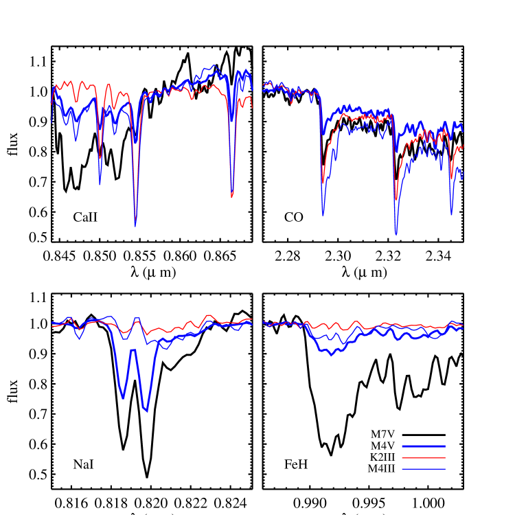
Figure 6.— IRTF spectra for stars of various spectral types and luminosity classes. The plots feature four surface gravity-sensitive and temperature-sensitive spectral features. The top panels highlight features that are strong in giants compared to dwarfs, while the bottom panels highlight features that are strong in dwarfs compared to giants. Spectra are normalized in order to highlight the gravity-sensitive lines. Notice in particular the two spectra that have the same spectral type (M4) but different luminosity class (V vs. III).

Table 1Definition of Spectral Indices

Index	Feature	Blue	Red	Notes
		Continuum	Continuum
	(Å)	(Å)	(Å)
CaII0.39	$3899.5-4003.5$	$3806.5-3833.8$	$4020.7-4052.4$	1
CN0.41	$4143.3-4178.3$	$4085.0-4097.6$	$4245.5-4285.5$	2
CaI0.42	$4223.5-4236.0$	$4212.2-4221.0$	$4242.2-4252.2$	2
CH0.43	$4282.6-4317.6$	$4267.6-4283.8$	$4320.1-4336.5$	2
FeI0.44	$4370.3-4421.6$	$4360.3-4371.6$	$4444.1-4456.6$	2
C20.47	$4635.3-4721.6$	$4612.8-4631.6$	$4744.1-4757.8$	2
FeI0.50	$4979.2-5055.4$	$4947.9-4979.2$	$5055.4-5066.7$	2
MgH0.51	$5070.5-5135.6$	$4896.5-4959.0$	$5302.6-5367.6$	2
FeI0.52	$5247.2-5287.2$	$5234.7-5249.7$	$5287.2-5319.7$	2
MgI0.52a	$5161.6-5194.1$	$5144.1-5162.8$	$5192.8-5207.8$	2
MgI0.52b	$5165.0-5220.0$	$5125.0-5165.0$	$5220.0-5260.0$	3
FeI0.53	$5313.6-5353.6$	$5306.1-5317.4$	$5354.9-5364.9$	2
NaI0.59	$5878.5-5911.0$	$5862.2-5877.2$	$5923.7-5949.7$	2
NaI0.82	$8177.0-8205.0$	$8170.0-8177.0$	$8205.0-8215.0$	3
CaII0.86	$8484.0-8513.0$	$8474.0-8484.0$	$8563.0-8577.0$	4,5
	$8522.0-8562.0$	$8474.0-8484.0$	$8563.0-8577.0$
	$8642.0-8682.0$	$8619.0-8642.0$	$8700.0-8725.0$
MgI0.88	$8801.9-8816.9$	$8777.4-8789.4$	$8847.4-8857.4$	6
TiO0.89		$8835.0-8855.0$	$8870.0-8890.0$	3,7
FeH0.99	$9905.0-9935.0$	$9855.0-9880.0$	$9940.0-9970.0$	3
NaI1.14	$11372-11415$	$11360-11370$	$11417-11427$	3
KI1.17	$11680-11705$	$11667-11680$	$11710-11750$	3,5
	$11765-11793$	$11710-11750$	$11793-11810$
AlI1.31	$13115-13165$	$13090-13113$	$13165-13175$	3
CaI1.98	$19770-19795$	$19740-19765$	$19800-19840$	3,5
	$19845-19880$	$19800-19840$	$19885-19895$
NaI2.21	$22047-22105$	$22035-22045$	$22107-22120$	3
CO2.30	$22932-22982$	$22860-22910$	$23020-23070$	3,5
	$23220-23270$	$23150-23200$	$23300-23350$

Note. — (1) Serven et al. (2005); (2) Lick-based index (Trager et al., 1998); (3) new index; (4) Cenarro et al. (2001); (5) Index with multiple features. In such cases the total EW is the sum of the individual EWs; (6) Diaz et al. (1989); (7) Index defined as a flux ratio between blue and red pseudocontinua.

We have made use of the ATLAS model atmosphere and spectrum synthesis package (Kurucz, 1970, 1993), ported to Linux by Sbordone et al. (2004). In particular, we used the ATLAS12 model atmosphere code, which utilizes the opacity sampling technique. The use of ATLAS12 for our purpose is relatively novel because we allow the opacity to vary with each elemental abundance variation. In previous work related to the response of spectral indices to individual abundance variations (e.g., Tripicco & Bell, 1995; Korn et al., 2005), a single opacity distribution function was used for all individual abundance variations. The atmospheres are plane-parallel and stationary. The standard mixing-length theory is adopted for the treatment of convection, and local thermodynamic equilibrium (LTE) is assumed.

Once the atmospheres are generated, the SYNTHE program (Kurucz & Avrett, 1981) is used to generate a very high resolution ($R=100,000$) spectrum for each star over the wavelength range $0.3\mu m<\lambda<3.0\mu m$. A microturbulent velocity of $V_{t}=2.0\ {\rm km\,s}^{-1}$ is adopted, independent of spectral type and luminosity. We have recomputed a subset of the models with $V_{t}=1\ {\rm km\,s}^{-1}$ in order to explore the sensitivity of the spectra to this parameter. This change in $V_{t}$ results in a sizable change in the equivalent widths of many features ($\approx 0.2-2$Å; see also Tripicco & Bell, 1995). We care only about the relative response of the models (see below), and this is much less effected by a change in $V_{t}$. For example, considering the response of the model spectra to a factor of two enhancement in iron abundance, the difference between $V_{t}=2\ {\rm km\,s}^{-1}$ and $1\ {\rm km\,s}^{-1}$ is less than 0.1Å  in equivalent width for all lines of interest.

The line data are critical for construction of realistic stellar atmospheres and spectra. We have adopted the atomic and molecular linelists available on Kurucz’s webpage, including the molecules H₂O, TiO, FeH, C₂, CH, CN, NH, SiO, SiH, OH, MgH, CO, and H₂. In particular, we use the TiO linelist from Schwenke (1998) and the H₂O linelist from Partridge & Schwenke (1997). The FeH linelist is from the work of Dulick et al. (2003), but with a partition function tabulated by Kurucz specifically for this project.

We have identified 20 points along the 13.5 Gyr isochrone shown in Figure 1 ranging from the tip of the RGB down to $\ T_{\rm eff}=3170$ K and log$(g)=5.05$, corresponding to a main sequence mass of $0.15M_{\odot}$. A synthetic spectrum is computed at each of these points for later use in the spectral synthesis. Model atmospheres for cooler dwarfs failed to converge. We therefore extrapolate our spectral library in $\ T_{\rm eff}$ to cooler dwarfs down to 0.08$M_{\odot}$. This approximation will have little impact on our results because we only use the model spectra to created integrated light spectra for a Chabrier IMF, for which stars with $0.08M_{\odot}<M<0.15M_{\odot}$ contribute $\approx 10^{-3}$ of the total flux. Notice that previous work (e.g., Tripicco & Bell, 1995; Korn et al., 2005; Serven et al., 2005) only considered two or three points along the isochrone in order to gauge the relative response of spectral features to changes in abundances.

In the present work we adopt the latest solar abundances from Asplund et al. (2009). These new abundances for C, N, O, and Ne are significantly lower than the old solar abundances of Anders & Grevesse (1989) and Grevesse & Sauval (1998). In particular, the new [O/H] abundance is 0.24 dex lower than the Anders & Grevesse (1989) abundances. This results in substantially better agreement between model spectra and data for late-type M dwarfs due to the resulting weaker H₂O opacity.

We have run models with individual abundance variations for C, N, Na, Mg, Si, Ca, Ti, Fe, and generic $\alpha-$elements, although in the present work we focus primarily on the elements C, Na, Ca, Fe, and $\alpha$. We have also run models with a factor of two variation in the total metallicity, $Z$, with abundance ratios fixed at their solar values. We vary each abundance both higher and lower than its canonical value. This is in contrast to previous work, which only increased the abundances of elements in order to gauge their effect on the spectrum.

2.5. Spectral indices

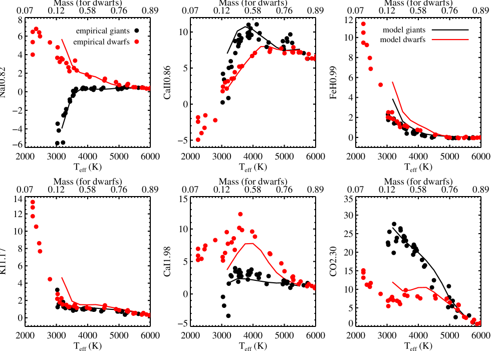
Figure 7.— Dependence of selected spectral indices on effective temperature for dwarfs (red points and lines) and giants (black points and lines). The empirical IRTF spectra (symbols) are compared to the model synthetic spectra (lines). At the top of each panel $\ T_{\rm eff}$ is converted into stellar mass for dwarfs via the isochrones discussed in $\S$2.2.

In later sections we will rely on spectral indices in order to investigate the sensitivity of various spectral features to the parameters age, metallicity, and IMF. Spectral indices have been utilized for decades to compress the amount of information in a spectrum. The most well-known are the Lick/IDS indices (Burstein et al., 1984; Worthey et al., 1994; Trager et al., 1998). These indices reside in the blue region of the spectrum ($4000$Å$<\lambda<6400$Å), and include indices sensitive to CN, C₂, CH, Ca, Cr, Fe, Mg, MgH, Na, and TiO (Tripicco & Bell, 1995; Korn et al., 2005). In the following work, we will utilize the Lick index wavelength intervals for the index bandpass and pseudocontinua as defined in Trager et al. (1998), but we make no effort to place our indices on the zero-point system of the Lick system. These indices are defined in Table 1. All indices in the present work (except for TiO0.89) are quoted as equivalent widths (EWs) with units of Å  (the procedure for measuring EWs is described in Worthey et al., 1994). All wavelengths in this paper are quoted in vacuum.

We supplement the Lick-based blue indices with additional indices as defined in Table 1. These indices were chosen for their promise in constraining the number of low mass stars from integrated light (in practice, we selected features that changed by more than 1% between a Chabrier and $x=3$ IMF; see Figure 10 below). The majority of the new indices are defined and measured in a manner analogous to the Lick-based indices. Exceptions include the calcium triplet (CaT) at $0.86\mu m$, which is comprised of three distinct features and so the total EW is the sum of the EWs of the individual features (see Cenarro et al., 2001, for details). Likewise, the CaI feature at $1.98\mu m$ is a doublet even when doppler broadened to $\sigma=300\ {\rm km\,s}^{-1}$, and so this feature is defined as the sum of two EWs. The CO index at $2.3\mu m$ is defined by the first two bandheads of the ¹²CO molecule. Finally, the TiO0.89 index is the only index defined as a ratio of fluxes between blue and red pseudocontinua, rather than an equivalent width.

The names given to the indices in Table 1 highlight the primary species controlling the strength of each index. In reality, each index is sensitive to a number of atomic and molecular species (see e.g., Tripicco & Bell, 1995; Korn et al., 2005, for details).

The use of indices suffers from several well-known problems. The EW of an absorption feature is measured with respect to a pseudocontinuum, which itself is composed of absorption features. The variation of an index due to changes in metallicity or age may therefore be due to a combination of changes in the feature itself and changes in the pseudocontinuum. Moreover, each index is in reality a blend of several absorption lines arising from more than one element. The spectral shape of the feature often contains additional information, beyond its EW, but this information is lost in an index. We will highlight these caveats in our results where applicable.

We emphasize that our use of indices in this work is restricted to “intuition-building” in the form of index-index plots — we do not advocate using indices when actually fitting data because of the limitations of indices highlighted above. The model spectra will be made available upon request so that others can measure their own indices and/or directly compare models to data at the appropriate resolution.

2.6. Behavior of the stellar libraries

Figure 6 shows surface gravity-sensitive spectral regions for selected IRTF stars. This figure highlights the potential power of certain spectral features at discriminating between dwarfs and giants. In this figure an M4 dwarf is compared to an M4 giant. These two stars have the same spectral type and thus broadly the same SED shape, but clearly have very different strengths of these spectral features. The M4 giant displays no FeH lines but instead shows TiO lines at almost the same wavelength as FeH. Also notice the dramatic increase in the FeH strength toward the latest M dwarfs. These stars also show very different features around the CaII lines compared to both slightly warmer dwarfs and giants. The different relative response of the NaI and FeH lines to later-type M dwarfs implies that these lines are sensitive to IMF variations in different ways.

In Figure 7 we show selected spectral indices as a function of effective temperature for giants and dwarfs. This figure compares the empirical IRTF spectra to the synthetic spectra. As expected, the indices NaI0.82 and FeH0.99 are stronger in dwarfs than in giants, and FeH0.99 becomes very strong for the coolest dwarfs. The CO2.30 and CaII0.86 indices also behave as expected in that they are stronger in giants than dwarfs. Notice though that the CO2.30 index becomes progressively stronger for dwarfs with $\ T_{\rm eff}<3000$ K (see Figure 6).

Two new spectral regions are explored in this figure: the KI doublet at 1.17$\mu m$ and the CaI doublet at 1.98$\mu m$. These features are both stronger in dwarfs than in giants, but they behave in very different ways. The KI1.17 index is even more sensitive to the very coolest stars than FeH0.99, while CaI1.98 peaks in strength at $\approx 3700$ K (corresponding to $\sim 0.55M_{\odot}$ for dwarfs).

It is noteworthy that the synthetic spectra reproduce the qualitative behavior of all the indices shown in Figure 7 and reproduce in detail the NaI0.82, CaII0.86, KI1.17, and CO2.30 indices. The models extend only to 3170K, so the models cannot be compared to the coolest M dwars. The synthetic spectra predict a CaII0.86 index stronger than observed for the coolest giants, which might be related to non-LTE effects, a FeH0.99 index stronger than observed for most dwarfs, which is probably due to problems with the FeH linelist and/or partition function, and a CaI1.98 index for dwarfs that is weaker than observed, which may be due to the fact that the pseudocontinuum is strongly affected by H₂O in this wavelength region.

The trends in this figure set the stage for the results to be discussed in $\S$4 and in particular $\S$4.4 where we discuss the ability of combinations of these indices to constrain the shape of the low-mass IMF in the integrated light of old stellar populations.

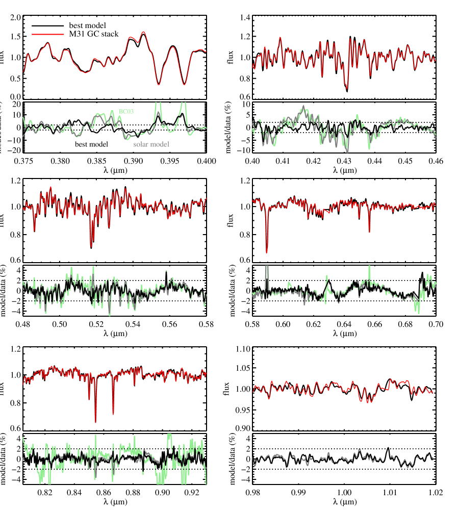
Figure 8.— Comparison of a stacked spectrum of four metal-rich M31 GCs to models. A best-fit model with variable abundance ratios (the “best model”), is compared to our solar metallicity model and the high-resolution solar metallicity model from Bruzual & Charlot (2003, BC03). Both model and data spectra were continuum normalized by a third-order polynomial within each wavelength interval. The bottom portion of each panel shows the ratio between model and data in percent units. The dotted lines demarcate a $\pm 2$% deviation. For the best-fit model, the deviations are less than 2% redward of $0.4\mu m$ and the root-mean-square deviation is 1.2%, testifying to the high fidelity of our models.

2.7. Synthesis

With the isochrones and stellar libraries described in previous sections we are now able to construct integrated light SSP spectra via Equation 1. We emphasize that the synthesis includes not only the RGB but also the HB and AGB. For a 13.5 Gyr solar metallicity population with a Chabrier IMF, stars on the HB and AGB comprise $\approx 25$% of the integrated light at $1\mu m$, so their inclusion in the synthesis is essential. When adding the HB and AGB we frequently used an empirical star that was already counted on the RGB. In such cases only the stellar mass is changed in accordance with the $\ L_{\rm bol}-M$ relation on the HB and AGB.

Abundance effects are implemented in a differential sense. This is the standard method of implementing abundance ratio effects in population synthesis (e.g., Trager et al., 2000; Thomas et al., 2003b; Schiavon, 2007; Walcher et al., 2009). The empirical stellar libraries constitute the base set of models, and the synthetic stellar libraries, which exist for arbitrary abundance patterns, are used to differentially change the base models. In practice, the model makes a prediction for an SSP spectrum of arbitrary abundance pattern $R$ via:

$$f(R)=f_{\rm base}\frac{f_{\rm syn}(R)}{f_{\rm syn}(Z_{\sun})},$$ (2)

where $f$ is the spectrum and we have implicitly assumed that the base empirical models have solar metallicity. Indices are then measured from these model spectra.

Our model thus provides SSPs for arbitrary IMFs, for stellar ages in the range $3-13.5$ Gyr, and for arbitrary elemental abundance patterns. We have avoided younger ages both because the IRTF library does not contain hot stars and because at younger ages thermally-pulsating AGB stars, whose evolution is highly uncertain, contribute significantly to the near-IR flux.

We have performed a number of tests to ensure that our resulting base model is not affected by one or more ‘pathological’ empirical stellar spectra. In addition to investigating each empirical spectrum by eye, we have constructed a set of models by removing one stellar spectrum at a time from the library and constructing a new SSP based on these $N-1$ spectra. The resulting indices never changed by more than 2% from our fiducial model. As will be shown in later sections, the index variations induced by modest variations in age, IMF, and abundances are always much larger than 2%. We conclude that our results are not unduly sensitive to any particular star in the empirical library.

3. A Brief Comparison to Data

In this section we briefly explore the quality of the models constructed in the previous section by comparing them to spectra of globular clusters (GCs). There are a number of massive metal-rich ([Fe/H]$\gtrsim-0.1$) ancient GCs in M31 (Caldwell et al., 2011). Such objects are ideal to compare to our models because our models are applicable to old metal-rich systems and because massive GCs will have a fully populated RGB. Red and near-IR spectra were obtained for the GCs B143, B147, B163, and B193 from the LRIS spectrograph on the Keck I telescope. These data were described in van Dokkum & Conroy (2011). Blue spectra were obtained from the Hectospec spectrograph on the MMT by Nelson Caldwell (unpublished). The spectra were stacked to create an average GC spectrum with typical signal-to-noise $>100$. There are significant sky subtraction issues in the wavelength regions $0.7\mu m<\lambda<0.8\mu m$ and $0.93\mu m<\lambda<0.98\mu m$ so those regions will be omitted in the following comparison.

Figure 8 shows the comparison between our models and the stacked M31 GC spectrum. Within each wavelength interval the spectra have been continuum normalized by a third-order polynomial. Our best-fit model was obtained via a Markov Chain Monte Carlo fitting technique with variation in each of the elements C, N, Na, Mg, Si, Ca, Ti, Fe, and with lock-step variation in the elements O, S, and Ne. The IMF is also varied, and the age is kept fixed at 13.5 Gyr. The data provide very strong constraints on the abundances of these elements and set a strong upper bound on the slope of the IMF. Discussion of the derived parameters is beyond the scope of this paper but is the focus of ongoing work.

The purpose of Figure 8 is to demonstrate the high quality of our models. The rms difference between the data and our best-fit model is 1%, and the percent difference at any wavelength point rarely exceeds 2% at $\lambda>0.4\mu m$. In this figure we also include comparison to our solar metallicity model, and the high-resolution solar metallicity model from Bruzual & Charlot (2003). Both of these models assume a Chabrier IMF. The solar metallicity models provide a reasonable fit to the data over much of the optical wavelength range, but at essentially every wavelength the best-fit model performs better. Regions where the best-fit model substantially outperforms the solar models include the CH and CN bands in the blue, the Mgb doublet at 0.52$\mu m$, the FeI lines at $0.48-0.54\mu m$, the NaD line at $0.59\mu m$, and the CaII triplet at $\sim 0.86\mu m$.

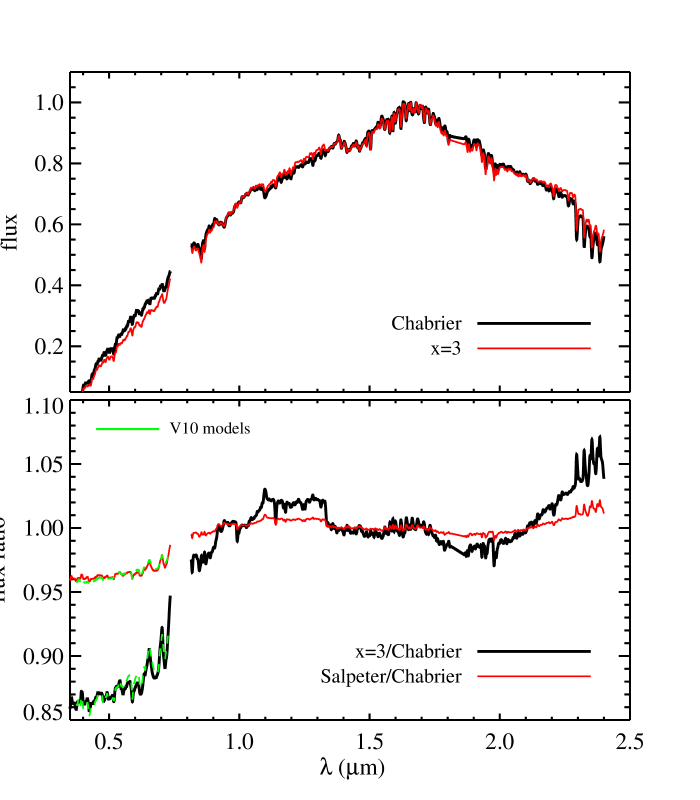
Figure 9.— Model spectra for solar metallicity and an age of 13.5 Gyr. Spectra are shown for three IMFs and have been smoothed by a Gaussian with FWHM$=40$Å  in order to highlight the broadband differences between models with different IMFs. The gap at $0.74-0.81\mu m$ is due to the gap in wavelength coverage between the empirical MILES and IRTF spectral libraries. Top panel: Comparison between models with a Chabrier and an $x=3$ IMF. Spectra are normalized to unity at 1.6$\mu m$. Bottom panel: Flux ratio between models with different IMFs, as indicated in the legend. Also shown are ratios of SSPs with different IMFs from Vazdekis et al. (2010, green lines).

Figure 10.— Ratio between a model spectrum with a Chabrier IMF and one with an $x=3$ IMF. The spectra are otherwise identical, both with an age of 13.5 Gyr and solar metallicity. The spectra are at the native resolution of the empirical libraries used to generate the models ($R\approx 2000$), and have been divided by a fourth-order polynomial in order to focus attention on the narrow-band features. Selected spectral features are labeled. Notice the different $y-$axis range in the upper left panel.

This figure demonstrates that the models we have constructed are capable of reproducing observed spectra at the percent level over the entire wavelength range of $0.37\mu m<\lambda<1.02\mu m$. This comparison also places strong limits on the presence of telluric lines in our model spectra because the M31 GC spectra are at different observed wavelengths than our empirical stellar library (The recession velocity of M31 is $-300\ {\rm km\,s}^{-1}$, which means that the GC spectra were shifted on average $5-10$Å  between the observed and restframe). Evidently, sky subtraction and sky absorption corrections have not introduced errors at the level $\gtrsim$1% in either the synthesized spectra or the M31 spectra.

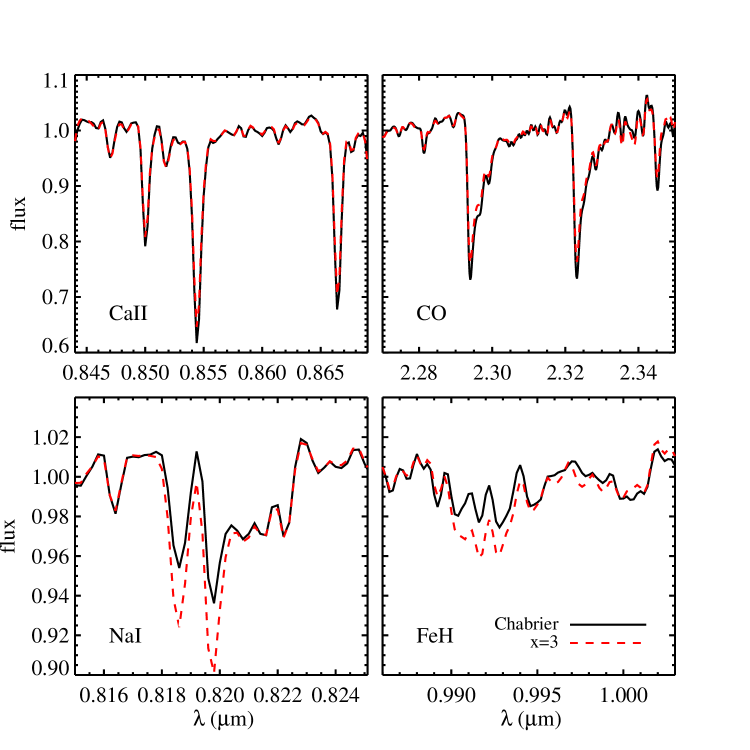
Figure 11.— Model spectra for four IMF-sensitive spectral features. Models are shown for an age of 13.5 Gyr, solar metallicity, and two IMFs: a Chabrier IMF and a bottom-heavy $x=3$ IMF. The dwarf-strong features are shown in the bottom panels, while the giant-strong features are shown in the top panels. Spectra have been divided through by a first-order polynomial (excluding the features of interest from the fit) in order to highlight the differences in the features.

4. Behavior of the Models

In this section we discuss how the models behave as a function of the IMF, stellar age, and elemental abundances. The goal of this section is to demonstrate that the integrated light spectrum of an old population is sufficient to jointly constrain the mean stellar age, metallicity, abundance pattern, and low mass IMF ($0.08M_{\odot}<M<1M_{\odot}$). All of the models presented in this section are SSPs — that is, they are coeval and mono-metallic. Throughout this section we frequently highlight the IMF-dependence of the integrated spectra by contrasting a Chabrier IMF with a relatively extreme bottom-heavy $x=3$ IMF. Also, in this section we rely on spectral indices in order to explore the behavior of the models. However, as discussed in $\S$2.5, we advocate using the spectra directly, rather than constructing indices, when fitting models to data.

4.1. Overview

Our models based on empirical stellar spectra are shown in Figures 9, 10, and 11. In this series of figures we explore the sensitivity of the SSP spectrum to the IMF, zooming in on smaller wavelength intervals with each successive figure. The age is fixed at 13.5 Gyr and the metallicity is solar.

In the top panel of Figure 9 we show the overall spectral energy distribution for two models that differ only in the adopted IMF. The bottom panel shows the ratio between spectra constructed with different IMFs. In both panels the spectra are normalized to unity at 1.6$\mu m$. The broad-band differences between a Chabrier IMF and a Salpeter IMF in the shape of the spectrum are slight, less than a few percent (see also Conroy et al., 2009). The differences become more substantial for a bottom-heavy IMF with $x=3$. In this case $I-z$ colors can differ by $>10$% in flux. We caution however that tying the IRTF spectra (which comprise the model predictions at $\lambda>0.81\mu m$) to the MILES spectra (which comprise the model predictions at $<\lambda<0.74\mu m$) relies on a heterogeneous compilation of $V-K$ colors that are probably not accurate to better than a few percent. The absolute broad-band model predictions should therefore be treated with some caution until the relative flux calibration between the MILES and IRTF libraries can be independently assessed.

In this figure we also include predictions from the models of Vazdekis et al. (2010, V10). These models adopt the MILES stellar library and the Padova isochrones in constructing SSPs. The models shown are of solar metallicity and have an age of 12.6 Gyr. For the V10 models we plot ratios between a Salpeter and Kroupa (2001) IMF, and between an $x=2.8$ and Kroupa IMF. The Kroupa IMF is essentially identical to the Chabrier IMF, and the $x=2.8$ IMF was the closest in their model grid to our $x=3$ IMF. Overall the agreement between our models and the V10 models is excellent. On a more refined level the agreement is even more impressive: after dividing the spectra by a second order polynomial and broadening by 5Å  (rather than the 40Å  shown in Figure 9), the models agree in the predicted spectral variation between a Salpeter and Chabrier IMF to a level of $\lesssim 0.2$%.

In Figure 10 we zoom in on the narrow spectral features by dividing the spectra in each wavelength interval by a fourth-order polynomial. The panels highlight the spectral response to a change in IMF when all other variables (age, metallicity) are held fixed. Selected spectral features are labeled. This figure summarizes all of the known surface gravity-sensitive lines in cool stars between $0.4-2.4\mu m$. The NaI082, CaII086, FeH099, and CO230 features are clearly visible. Additional, less well-known lines are also clearly visible, including NaI, KI, AlI, and CaI, all of which are stronger in dwarfs than giants. The numerous lines from CO in the $H-$band are also visible.

As noted in $\S$2.3, the faintest M dwarfs in our empirical library display strong chromospheric emission lines, particularly the hydrogen Balmer series and the CaII H & K lines at $0.39\mu m$. In the upper left panel of Figure 10 we see that the H$\alpha$ and CaII lines display strong IMF sensitivity. Approximately one half of the effect is due to chromospheric emission in the latest M dwarfs in our sample. In fact, we expect the true effect to be even larger, since our sample of optical M dwarf spectra only extends to spectral type M7. The remaining one half of the IMF effect in these lines is simply due to the fact that these features in absorption are weaker in M dwarfs compared to other stars.

Figure 11 zooms in further on four classic IMF-sensitive spectral features. The spectra have been divided by a first-order polynomial to focus attention on the features. It is evident from this figure that the differences in flux between a Chabrier and an $x=3$ IMF in these features are of order several percent. Differences between a Chabrier and Salpeter IMF (not shown) are of order one percent. This figure demonstrates that very high $S/N$ spectra are required in order to differentiate between IMFs based on these features.

In this section we have summarized the basic trends evident in our models based on empirical stellar spectra. These models confirm a wide array of previous work that the low-mass IMF, or phrased another way, the ratio of M giants to M dwarfs, can be inferred directly from integrated light spectra of old populations. The fundamental uncertainty in any modeling approach is the interplay between the IMF, average stellar age, and abundance pattern. In the following section we address this issue in detail.

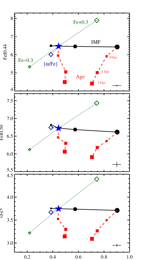
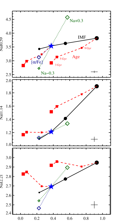
Figure 12.— Variation in the EW of spectral indices involving the elements iron (left panel) and sodium (right panel). The panels show the effect of varying the IMF (bottom-light, Chabrier, Salpeter, $x=3$; solid lines), elemental abundance ([Fe/H] or [Na/Fe], and [$\alpha$/Fe]; dotted lines) and stellar population age (3,5,9,13.5 Gyr; dashed lines). The model iron and sodium abundances vary by $\pm 0.3$ dex and the model $\alpha-$enhancement varies from $0.0-0.2$ dex. Changes in age are only shown with respect to the Chabrier and $x=3$ IMFs for clarity. The symbol size increases toward steeper IMFs, higher metallicity, and younger ages. The blue star represents the fiducial model of a 13.5 Gyr solar metallicity population with a Chabrier IMF. The EWs are in Å. Typical measurement uncertainty of each index is shown in the lower portion of each panel, assuming a signal-to-noise of $S/N=200$ Å^-1 and $R\approx 2000$.

4.2. Variation in IMF, age, and elemental abundances

In this section we combine our model predictions based on empirical stellar libraries with the synthetic stellar libraries described in $\S$2.4. We explore the dependence of a suite of spectral indices on stellar age, abundance pattern, total metallicity, and IMF, focusing on indices governed by iron, sodium, calcium, carbon, and magnesium. In particular, we explore variations in age between $3-13.5$ Gyr, IMFs between a bottom-light, Chabrier, Salpeter, and $x=3$, $\alpha-$enhancement between $0.0<$[$\alpha$/Fe]$<0.2$, and individual elemental abundance variation. Notice that the abundance variations of calcium, carbon, sodium, and $\alpha-$enhancement were implemented at fixed [Fe/H] and so [e/H]$\equiv$[e/Fe] where “e” refers to generic elemental abundance. This also implies that the total metallicity, $Z$, varies from model to model. The red spectra are sensitive to age in the range we consider ($3-13.5$ Gyr) primarily because of the increased contribution of M giants to the integrated light at younger ages. The hotter main sequence turn-off point at younger ages has a larger impact on the blue spectrum.

4.2.1 Iron

The left panel of Figure 12 shows iron-sensitive spectral indices. The composite index $\langle$Fe$\rangle\equiv 0.5($FeI$0.52+$FeI$0.53)$ was defined by Trager et al. (2000) and is used extensively in the literature. The figure shows the response of these indices to changes in the IMF, stellar age, and abundance pattern. The iron abundance, [Fe/H], varies by $\pm 0.3$ dex. We also incude measurement uncertainties on each index assuming a signal-to-noise ratio per angstrom of $S/N=200$ Å^-1.

An important feature of these index-index plots is that the effects of the IMF are nearly orthogonal to both age and abundance effects. The insensitivity of FeH to ages ¿5 Gyr for a Chabrier IMF found here is in agreement with previous work (Couture & Hardy, 1993; Schiavon et al., 2000). The response of the blue indices (along the y-axes) to age, [$\alpha$/Fe], and [Fe/H] are well-known (e.g., Schiavon, 2007). In particular, the FeI0.44 index weakens with increasing [$\alpha$/Fe] due to the increased presence of magnesium and calcium lines in the index pseudocontinuum (Schiavon, 2007).

The insensitivity of the FeH index to [$\alpha$/Fe] is a key result of this paper. This result is at first glance surprising, given the fact that TiO absorption in M giants coincides with the index bandpass for FeH (see Figure 6), and Ti and O are both $\alpha-$elements. In fact, the strength of the TiO feature at 0.99$\mu m$ is almost entirely insensitive to 0¡[$\alpha$/Fe]$<0.2$ because of two unrelated effects. First, the atmospheric structure changes with increased [$\alpha$/Fe] in such a way so as to significantly diminish the effect of increased abundance of TiO on the TiO linestrength. This is confirmed by computing a set of synthetic spectra where the atmospheres were computed at solar abundances but the spectra were created with [$\alpha$/Fe]$=0.2$. In this case the TiO features increase with $\alpha-$enhancement. The second effect causing the FeH0.99 index to be insensitive to the TiO abundance is the fact that the TiO feature at 0.99$\mu m$ sits atop a much larger TiO feature whose band-head is at $0.97\mu m$ (both are part of the $\delta$ system). The strength of the TiO feature at 0.99$\mu m$ is determined by the ratio of the line opacity to the pseudocontinuum, both of which scale with the abundance of TiO. For these reasons the TiO feature at 0.99$\mu m$ feature is quite insensitive to TiO abundance.

Notice that while the FeH0.99 index is insensitive to ages of ¿5 Gyr for a Chabrier IMF, it becomes increasingly sensitive to age for steeper IMFs. This is a consequence of the fact that at younger ages M giants contribute more to the integrated flux, so they outshine the M dwarfs. This dependence of FeH0.99 on age is an important prediction of any model that ascribes a bottom-heavy IMF to a particular stellar population. In other words, if a certain class of objects, say massive ellipticals, were thought to possess a bottom-heavy IMF, then one should find a strong correlation between the mean stellar age and FeH0.99 strength within that population. For a standard Chabrier IMF, no such correlation should exist for ages $>5$ Gyr. This prediction is unique to the FeH0.99 index. As will be shown in later sections, all other IMF-sensitive lines that we consider show correlations with age for both Chabrier and bottom-heavy IMFs.

The results in this section show that the combination of any blue iron-sensitive index with the near-IR FeH index should provide an unambiguous separation of the effects of the IMF from abundance and age effects.

4.2.2 Sodium

The right panel of Figure 12 shows sodium-sensitive spectral indices as a function of the IMF, stellar age, and abundance pattern. The sodium abundance, [Na/Fe], varies by $\pm 0.3$ dex.

All sodium-sensitive indices weaken with increasing [$\alpha$/Fe] due to the fact that the pseudocontinua are strongly influenced by $\alpha-$elements. The NaI0.82 index decreases with decreasing age, in agreement with previous work (Schiavon et al., 2000). The NaI0.59 index (also known as NaD) is in theory a useful line because it responds much more strongly to [Na/Fe] than the IMF. Unfortunately, this index is influenced by the interstellar medium (ISM; of the system in question and, for systems at zero redshift, the Galaxy), and so interpretation of this index is quite complicated. The NaI1.14 index is very sensitive to the IMF, as is the NaI0.82 index, although it is also sensitive to [Na/Fe]. Both of these indices scale in the same way with [Na/Fe] and IMF, implying that they cannot be used in isolation to jointly constrain the IMF and sodium abundance. The NaI2.21 and NaI0.82 indices separate the effects of abundance and IMF somewhat more cleanly.

For late-type giants sodium is the third most important electron contributor at a Rosseland mean opacity of order unity, after Mg and Al, while for late-type dwarfs it is the most important, followed by Ca. The abundance of sodium therefore affects the strength of many other features through its influence on the electron pressure. For example, increasing the sodium abundance causes a decrease in the abundance of CaII, which causes a decrease in the EW of CaII0.86. The importance of this effect should not be underestimated. Specifically, an increase in [Na/Fe] by 0.3 dex causes a decrease in the EW of CaII0.86 of 1.6%. Compare this to the decrease in CaII0.86 of 3.1% between a Chabrier and Salpeter IMF. It is therefore essential to consider not only IMF-sensitive indices such as NaI0.82 and CaII0.86 but also indices that are sensitive to [Na/Fe] in order to separate the effects of [Na/Fe] from the IMF. It is however worth noticing that while an increase in [Na/Fe] can cause an increase in NaI0.82 and a decrease in CaII0.86, mimicking the effects of a more bottom-heavy IMF, quantitatively a very large increase in [Na/Fe] would be required (at least 0.6 dex) to mimic an $x=3$ IMF in these indices.

In summary, unlike the iron-sensitive indices, the situation with sodium is more complex. Were it not for the influence of the ISM on the NaI0.59 index, the combination of this index with NaI0.82 would provide a powerful means for separating the IMF from other effects. The red and near-IR sodium-sensitive indices respond strongly and positively to both [Na/Fe] and IMF variations, making it difficult to use these lines alone to separate IMF effects from others. An independent constraint of the sodium abundance would make the near-IR sodium lines powerful IMF diagnostics.

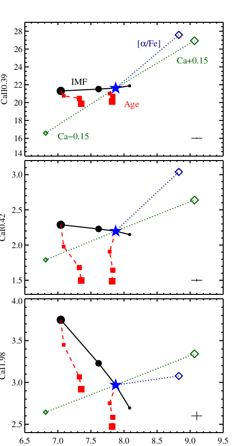
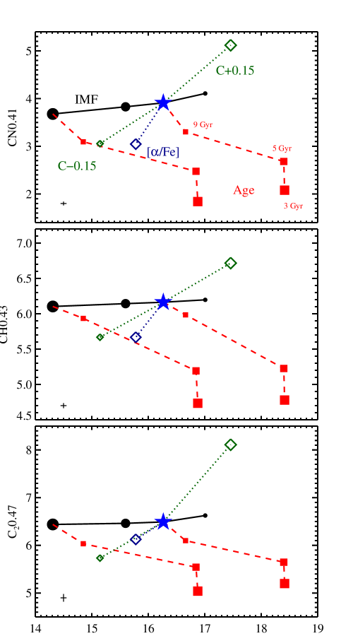
Figure 13.— Same as Figure 12, now for calcium (left panel) and carbon (right panel). The model carbon and calcium abundances vary by $\pm 0.15$ dex.

4.2.3 Calcium

The left panel of Figure 13 shows calcium-sensitive spectral indices as a function of the IMF, stellar age, and abundance pattern. The calcium abundance, [Ca/Fe], varies by $\pm 0.15$ dex.

The well-known IMF-sensitive CaII0.86 index (also known as the calcium triplet or CaT) is shown here to be weakly sensitive to age, in agreement with previous work (Schiavon et al., 2000; Vazdekis et al., 2003), and strongly sensitive to both [Ca/Fe] and [$\alpha$/Fe]. Since calcium is an $\alpha-$element, this latter fact is no surprise.

The CaII0.39 index (also known as the CaII H & K lines) is mildly sensitive to the IMF although it is difficult to gather this from Figure 13 because of the large $y-$axis range. The difference between a Chabrier and $x=3$ IMF is only 0.2Å. This index is very strongly sensitive to [Ca/Fe] and [$\alpha$/Fe] variations (see also Serven et al., 2005; Worthey et al., 2011). The much larger sensitivity of this index to abundances than the IMF suggests that it is useful primarily as an abundance indicator. The CaI0.42 index behaves in a similar way, although the change in the EW induced by abundance changes is much less dramatic. The CaI1.98 index increases significantly for more bottom-heavy IMFs. This index is proportionally much more sensitive to the IMF than abundance compared to other calcium-sensitive indices.

The combination of the CaII0.39 or CaI0.42 indices, which are primarily sensitive to calcium abundance, with both the CaI1.98 and CaII0.86 indices, which respond strongly and in opposite ways to changes in the IMF, should provide a strong constraint on the IMF.

4.2.4 Carbon

The right panel of Figure 13 shows carbon-sensitive spectral indices as a function of the IMF, stellar age, and abundance pattern. The carbon abundance, [C/Fe], varies by $\pm 0.15$ dex. The carbon abundance cannot increase much beyond 0.15 dex because a C/O ratio greater than unity would produce carbon stars, which are not expected to occur in old stellar populations (Renzini & Voli, 1981).

The classic surface gravity-sensitive CO2.30 index is shown here to be sensitive to the IMF, [C/Fe] abundance, age, and $\alpha-$enhancement. The index increases with decreasing age, meaning that an increasingly bottom-heavy IMF can be easily separated from age effects. A decrease in carbon abundance by 0.15 dex mimics a shift from a Chabrier IMF to an IMF in between Salpeter and $x=3$. CO decreases with increasing [$\alpha$/Fe] because the atmospheric structure changes in such a way as to decrease the CO2.30 EW. The abundance of CO is determined by carbon, which is less abundant than oxygen in the atmospheres of stars comprising old stellar systems, and so CO is less sensitive to O (an $\alpha$-element) than one may have otherwise supposed.

The blue carbon-sensitive indices CN0.41, CH0.43, and C₂0.47 are all very weakly sensitive to the IMF but are strongly sensitive to age, [C/Fe], and [$\alpha$/Fe]. These indices become weaker with increasing $\alpha-$enhancement because increasing [$\alpha$/Fe] increases the oxygen abundance, and, since CO has the highest dissociation energy, more oxygen means more carbon locked up in CO, which means less carbon available for CN and CH (Serven et al., 2005; Schiavon, 2007). C₂0.47 is doubly sensitive to carbon abundance for the obvious reason that it is composed of two carbon atoms.

The combination of any of the blue carbon-based lines with the CO2.30 index should provide a strong constraint on both the IMF, stellar age, and elemental abundances.

4.2.5 Magnesium

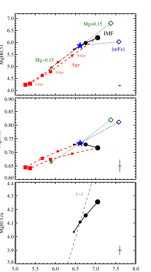
Figure 14.— Same as Figure 12, now for magnesium. The model magnesium abundances vary by $\pm 0.15$ dex. The bottom panel compares the classic Mgb Lick index (MgI0.52a) with our new MgI0.52b index. A line with unity slope (dashed line) is shown for comparison. Notice that our new index is considerably more IMF-sensitive than the standard Lick index. The MgH0.51 index, which is analogous to the Mg₁ Lick index, also displays some sensitivity to the IMF.

Magnesium spectral features have played a central role in our understanding of the abundance patterns of old stellar systems. For example, the Mgb feature (consisting of a triplet of MgI lines at $0.52\mu m$) has been used extensively to measure [$\alpha$/Fe] in elliptical galaxies (with the key assumption that Mg traces $\alpha$; e.g., Worthey et al., 1992; Trager et al., 1998; Thomas et al., 2005; Schiavon, 2007). The importance of magnesium in stellar population studies has motivated us to consider this element in the context of our models.

In Figure 14 we consider four magnesium-sensitive features. The MgH0.51 index (equivalent to the Mg₁ Lick index) is very sensitive to [Mg/Fe] and moderately sensitive to age and the IMF. Interestingly, it is insensitive to [$\alpha$/Fe]. The near-IR MgI line measured by the MgI0.88 index is sensitive to [Mg/Fe] and [$\alpha$/Fe], in agreement with previous work (e.g., Diaz et al., 1989; Cenarro et al., 2009). It is a weak feature, requiring very high $S/N$ spectra to obtain a useful measurement, and it is insensitive to the IMF for reasons described below.

The strength of the Mgb lines are quantified herein with two indices: the MgI0.52a index (equivalent to the Mgb Lick index), and the MgI0.52b index. The latter index is new and was constructed to be maximally sensitive to the IMF. This is clearly demonstrated in the bottom panel of Figure 14. The MgI0.52a index changes by 0.16Å  between a Chabrier and $x=3$ IMF, compared to 0.46Å  for the MgI0.52b index. The reason for this difference is due to a triplet of CrI lines centered at $\approx 5208$Å, and blended with FeI, TiI, and MgH lines, that becomes stronger with decreasing $\ T_{\rm eff}$ and hence stronger for steeper IMFs. The CrI blend partially overlaps with the red pseudocontinuum bandpass of the Lick Mgb index, and so the IMF-sensitivity of that index is greatly reduced. Our new index includes the CrI blend in the index definition, thereby enhancing the effect of the IMF on the index. We emphasize that using the full spectrum to estimate the IMF, abundance, age, etc., rather than spectral indices, would circumvent these complications.

There are several additional effects responsible for the IMF trends of these indices (see e.g., Schiavon et al., 2004; Schiavon, 2007). For $\ T_{\rm eff}>4000$K, the strengths of MgH0.51, MgI0.52a, and MgI0.52b increase with decreasing $\ T_{\rm eff}$ and increasing log($g$). These trends can be attributed primarily to the increasing strength of the MgH and MgI spectral features. At cooler temperatures TiO bands have a significant, and eventually dominant, influence on these indices. One TiO bandhead overlaps almost perfectly with the Mgb lines. The fact that at $\ T_{\rm eff}<4000$K the Mgb Lick index becomes primarily a measure of TiO, combined with the fact that TiO bands are stronger in giants than in dwarfs, led Schiavon (2007) to conclude that this index should not be sensitive to the IMF. While it is true that the Lick Mgb index is fairly weakly sensitive to the IMF, it is primarily because of contamination by the CrI blend in the red pseudocontinuum. Indeed, our refined MgI0.52b index shows significantly stronger IMF-dependence. Although the TiO bands are not as strong in dwarfs compared to giants, they are still sufficiently strong to affect the Mgb region when the number of dwarfs is increased.

Finally, the MgI0.88 index is almost completely insensitive to the IMF in part because there is very little dependence of this feature on log($g$) at fixed $\ T_{\rm eff}$ (Cenarro et al., 2009). This index peaks in strength for $4000{\rm K}<\ T_{\rm eff}<4500$K, becoming weaker at both higher and lower $\ T_{\rm eff}$. At the very coolest temperatures ($\ T_{\rm eff}<3000$K) the dwarfs do show stronger MgI0.88 than giants (due to an unidentified feature at $\approx 8800$Å), but the strength is comparable to K giants, and so the addition of late M dwarfs does not leave a signature on this index in the integrated light.

In summary, there is some sensitivity to the IMF in the Mgb spectral region. In this spectral region the use of indices greatly complicates the interpretation of model variations. Direct manipulation of the model spectra has provided some clarity. This serves as yet another argument in favor of our position that model and data should be compared directly in spectral space, rather than in index space. Finally, we draw attention to the fact that, while the MgI0.52b feature displays a moderate degree of IMF sensitivity, it is not an ideal probe of the IMF. This is because the IMF sensitivity is due largely to the influence of TiO, which, in the absence of any prior on the isochrones, can be due to either dwarfs or giants. In other words, we could have added more M giants rather than M dwarfs, which would have increased the strength of TiO in the model, and thereby the strength of MgI0.52b. We return to this point in $\S$4.3.

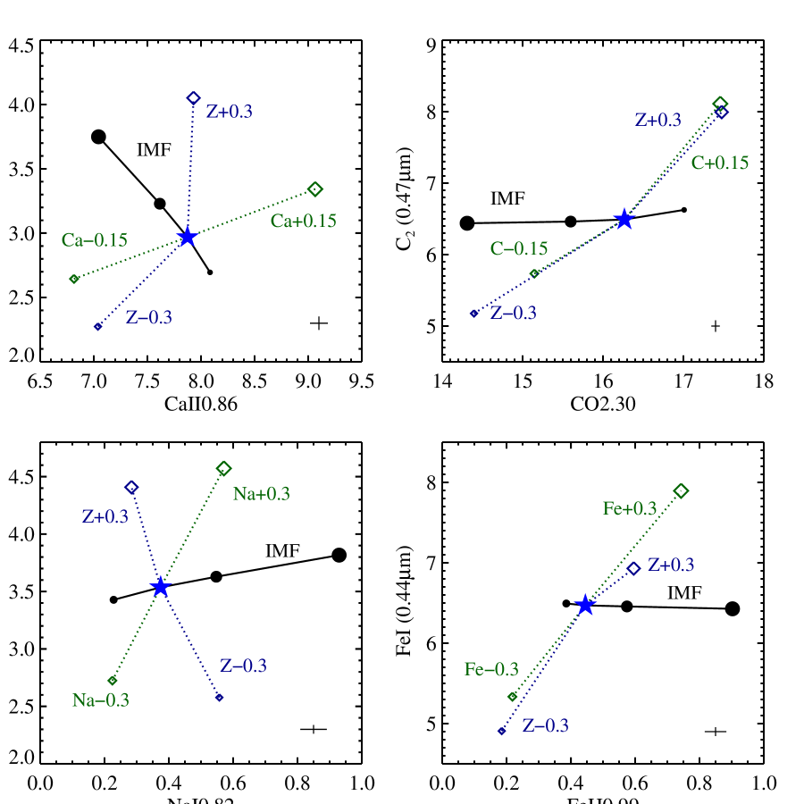
Figure 15.— Effect of metallicity, $Z$, on spectral indices. Each panel highlights the effect on indices dominated by a single element (cf. Figures 11-12). The effect of metallicity variation of $\pm 0.3$ dex is compared to variation in the abundance of a single element, and to the IMF. The carbon and calcium abundance varies by $\pm 0.15$ dex while the sodium and iron abundance varies by $\pm 0.3$ dex. Symbol size increases toward higher abundances, higher metallicities, and steeper IMFs. Error bars are as in Figures 11-12.

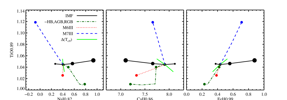
Figure 16.— Response of selected spectral features to variation in the number and type of luminous giants and the IMF. Models are constructed by removing the horizontal and asymptotic giant branches and also removing the most luminous RGB stars (dark green dashed lines), adding an increasing number of M6III (red dashed lines) or M7III (blue dashed lines) stars, and shifting the overall isochrone by $\pm 50$K (light green solid lines). Models with a varying IMF are also shown (black solid lines). Indices along the $x-$axis are measured in EW in Å  while the Ti0.89 index is measured as a flux ratio.

4.2.6 Total metallicity

In Figure 15 we explore the effect of varying the total metallicity, $Z$, on selected indices. In this case the abundance ratios are fixed to their solar values. In this figure we have selected a promising pair of indices that may yield IMF constraints for each of the four elements discussed in the previous sections. The metallicity is varied by $\pm 0.3$ dex.

The effect of metallicity variation on the indices is difficult to interpret because the abundance of every element is changing. In general not only will the flux in the central bandpass change but also the pseudocontinua used to define the index. As an example, the NaI0.82 index decreases with increasing metallicity because of increased TiO absorption in the red pseudocontinuum. In contrast, the CO2.3 index responds to carbon abundance variation and metallicity variation in very similar ways because the change in metallicity does not substantially change the pseudocontinuum, and so the change in CO abundance is the dominant effect. The same is true for the iron indices shown in the figure. The CaII0.86 index decreases with decreasing metallicity because of a change in the pseudocontinuum at $\approx 0.864\mu m$. The independence of CaII0.86 on $Z$ for super-solar metallicities has been noticed before by Vazdekis et al. (2003). These examples highlight the difficulty in using and interpreting indices. At this point we remind the reader that our use of indices in this paper is for illustrative purposes only. We do not advocate using them when fitting models to data, in part for the reasons discussed in this section.

The primary conclusion to be drawn from Figure 15 is that IMF variation cannot be confused with metallicity variation. In other words, the vectors of metallicity and IMF variation are largely orthogonal in these index-index plots.

4.3. Modifications to the fiducial isochrone

Our goal has been to demonstrate to what extent the effects of the IMF can be isolated from other effects on the integrated spectrum of old stellar populations. In the previous section we demonstrated that by employing a variety of spectral indices one can separate the effects of the IMF from the stellar age and abundance pattern. Apart from these changes to the characteristics of the stellar population, we also need to explore changes to the assumptions that go into the models, and in particular the precise location of the isochrones in the HR diagram and the weights assigned to giants in the stellar population synthesis.

We have identified three distinct isochrone-related effects that can mimic a change in the IMF via their impact on one or more of the IMF-sensitive indices NaI0.82, CaII0.86, and FeH0.99. These effects are 1) decreasing the number of luminous giants; 2) increasing the contribution from very late M giants; 3) shifting the location of the isochrone in the HR diagram. We explore these effects in Figure 16 where the IMF-sensitive indices are plotted against the TiO0.89 index, which is sensitive to both surface gravity and temperature (Carter et al., 1986; Cenarro et al., 2009). Similar index-index plots were used by Cenarro et al. (2003) to separate IMF effects from metallicity effects. Standard models are shown for IMFs ranging from Chabrier to Salpeter to $x=3$ (these are the same models shown in Figures 12 and 13).

We first consider the effect of decreasing the number of luminous giants with respect to a fiducial model with an age of 13.5 Gyr, solar metallicity, and a Chabrier IMF. Clearly this effect should mimic the effect of a bottom-heavy IMF to some extent since the IMF-sensitive indices only provide a measurement of the ratio of dwarfs to giants. The green line in Figure 16 shows the effect of first removing all HB and AGB stars, and then removing all stars at progressively lower RGB luminosities down to $\ L_{\rm bol}=10^{2}\ L_{\sun}$. This effect clearly mimics a bottom-heavy IMF in the NaI0.82 and CaII0.86 indices, but not the FeH0.99 index. The reason for this is because the FeH feature is only strong in the very lowest-mass M dwarfs, which contribute essentially no flux for a Chabrier IMF. Removing the giants actually causes a decrease in the FeH0.99 index because this index also measures the strength of a TiO absorption feature that occurs in late-type giants. The TiO absorption is a strong function of temperature, so removing the coolest giants causes a decrease in the TiO strength, and hence the FeH0.99 index. From Figure 16 it is clear that even for the NaI0.82 and CaII0.86 features, one can discriminate between a paucity of giants and a bottom-heavy IMF by considering the strength of the TiO0.89 index.

The next effect we consider is adding more weight to very cool giants than stellar models predict for an age of 13.5 Gyr. Specifically, we add increasing amounts of an M6III spectrum and an M7III spectrum to our fiducial model. At a maximum we include six times as many of these giants as a 13.5 Gyr isochrone would predict. Here again the addition of these cool giants can in principle mimic a bottom-heavy IMF for one or more (but not all three simultaneously) of the IMF-sensitive features shown in Figure 16. The addition of cool giants mimics a bottom-heavy IMF because these stars have very strong TiO absorption features that overlap with the FeH0.99 index and partially overlap with the NaI0.82 feature. The M7III actually weakens the NaI0.82 index because it provides substantial TiO absorption in the red pseudocontinuum of this index, thereby decreasing the EW. The CaII absorption at 0.86$\mu m$ weakens for the coolest giants, explaining the trends in that index as well (this is simply a consequence of ionization equilibrium; see Figure 7). However, as with the removal of RGB stars, consideration of these IMF-sensitive indices with the giant-sensitive TiO0.89 feature allows one to unambiguously distinguish between the addition of M giants and a bottom-heavy IMF.

Finally, we consider the effect of shifting the isochrone in temperature by $\pm 50$K. Such a shift can be caused for example by a change in [$\alpha$/Fe] by $\pm 0.2$ or [Fe/H] by $\pm 0.1$ dex (e.g., Dotter et al., 2007, 2008). We have modeled this effect by running a new set of synthetic stellar spectra with $\ T_{\rm eff}$’s offset by $\pm 50$K compared to the fiducial set. These new models were then used differentially to quantify the effect of changing the $\ T_{\rm eff}$ of all stars in the synthesis. The result is shown in Figure 16. Qualitatively, the effect is similar to adding/removing cool giants. The behavior of the TiO0.89 and FeH0.99 features with varying $\ T_{\rm eff}$ is due to the influence of TiO (for the reasons noted above). The CaII0.86 feature is sensitive to $\ T_{\rm eff}$ because of ionization equilibrium. It is noteworthy that the NaI0.82 feature is almost completely insensitive to $\pm 50$K changes to $\ T_{\rm eff}$. Overall, the impression from Figure 16 is that the effects of changing $\ T_{\rm eff}$ should be separable from an IMF effect.

The preceding discussion serves to highlight another limitation of the use of spectral indices — as opposed to the full spectrum — to chart IMF variations. Because cool stars contribute TiO to the indices NaI0.82 and FeH0.99 that have central wavelengths and line profiles that differ from NaI and FeH, the detailed spectral shape around these features can also provide a strong constraint on the contribution of cool giants to the integrated flux.

We mention a final point regarding the arbitrary addition or subtraction of luminous giants. In addition to the fact that stellar evolution dictates how many such giants there should be, direct constraints on the relative number of luminous giants come from surface brightness fluctuations (SBFs) measured in nearby galaxies (e.g., Tonry et al., 2001; Liu et al., 2002; Jensen et al., 2003). Results from SBFs do not allow for substantial deviation from the basic predictions of stellar evolution along the RGB and AGB. In any event, constraints from SBFs will provide a powerful independent test of any purported excess or deficit of luminous giants.

We conclude that the effects considered in this section imprint signatures not only on the IMF-sensitive features but also on the cool giant-sensitive TiO0.89 index. Moreover, no single effect considered in Figure 16 can simultaneously mimic an IMF effect in all three IMF-sensitive indices. These effects should therefore be separable from an IMF effect given a sufficient amount of spectral coverage. The detailed spectral shapes of the IMF-sensitive features will also provide a strong constraint on the contribution of cool giants to the integrated light.

4.4. Constraining the shape of the low-mass IMF

As was alluded to in $\S$2.6, the combination of multiple surface gravity-sensitive spectral indices should provide a constraint on the shape of the low-mass IMF in old stellar populations. This is possible because each spectral feature responds to changes in surface gravity and/or temperature in different ways (see Figure 7). The possibility of constraining the shape of the IMF in this way was already mentioned in Faber & French (1980).

The sensitivity of indices to the low-mass IMF is explored in Figure 17. In this figure we show the fractional change in each index as the weight applied to each mass interval is doubled. The change is computed with respect to a model with an age of 13.5 Gyr, Salpeter IMF, and solar metallicity. Models constructed from the empirical spectral libraries were used. The FeH0.99 and KI1.17 indices are the most sensitive to very low mass stars ($\lesssim 0.3M_{\odot}$), while the CaI1.98 and AlI1.31 indices are sensitive primarily to $0.4M_{\odot}\lesssim M\lesssim 0.7M_{\odot}$. The sensitivity of the NaI0.82 index is bracketed by these two extremes. While not shown, the giant-strong indices CaII0.86 and CO2.30 have a much weaker dependence on mass and never exceed a fractional change of 0.15 for any mass interval.

An example showing that it is possible to measure the shape of the low-mass IMF with these indices is shown in Figure 18. In this figure we show two indices as a function of the shape of the IMF. The dashed lines show variation in these indices for a varying logarithmic power-law index $x$ and fixed low-mass cutoff, $m_{c}=0.08M_{\odot}$, while the solid lines show variation in $m_{c}$ for a fixed logarithmic slope $x=3.0$. As expected, FeH0.99 responds most quickly to changes in the low-mass cutoff while CaI1.98 responds very weakly until $m_{c}>0.2M_{\odot}$. For $m_{c}>0.4M_{\odot}$ CaI1.98 responds strongly while FeH0.99 responds weakly, again as expected. Changes in the logarithmic slope result in a different relation between these indices.

Of course, the differences induced by different IMF shapes are more subtle than overall changes in the low-mass star content. Constraints on the shape of the IMF will therefore only be possible after the blue and red indices are used to jointly constrain the detailed abundance pattern and mean stellar age. Once these variables are known one may profitably use the gravity-sensitive indices to probe the detailed shape of the low-mass IMF in the integrated light of old stellar populations.

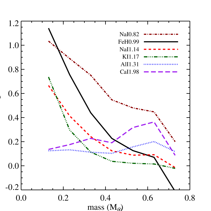
Figure 17.— Sensitivity of selected spectral indices to stellar mass. The fractional change in each spectral index is computed by doubling the number of stars in each mass interval. The index changes are computed with respect to a model with an age of 13.5 Gyr, solar metallicity, and Salpeter IMF.

4.5. Practicalities: Measuring the IMF with real data

In this section we comment on several practical aspects regarding the measurement of IMF-sensitive spectral features. We focus on the effect of velocity broadening, the required $S/N$, and the sky subtraction and flux calibration.

In the foregoing sections we presented results derived from spectra at their native resolution ($R\approx 2000$, or $\sigma\approx 64\ {\rm km\,s}^{-1}$). Figure 19 shows the extent to which the IMF sensitivity of selected spectral features is affected by increasing the velocity dispersion (due either to lower resolution data or an intrinsically higher velocity dispersion population). The figure shows the absolute change in an index between a Chabrier and $x=3$ IMF as a function of velocity dispersion. Not surprisingly, the difference decreases toward higher $\sigma$, and the effect is stronger for the CaII0.86 and NaI0.82 indices, which are relatively narrow features (see also Vazdekis et al., 2003). The FeH0.99 index is relatively insensitive to changes in $\sigma$ because this index is dominated by broad molecular features (FeH in dwarfs and TiO in giants). It is reassuring to note that while the signal is somewhat lower at high dispersion, the differences between a bottom-heavy and Chabrier IMF are still substantial even at $\sigma=300\ {\rm km\,s}^{-1}$ (see also van Dokkum & Conroy, 2010).

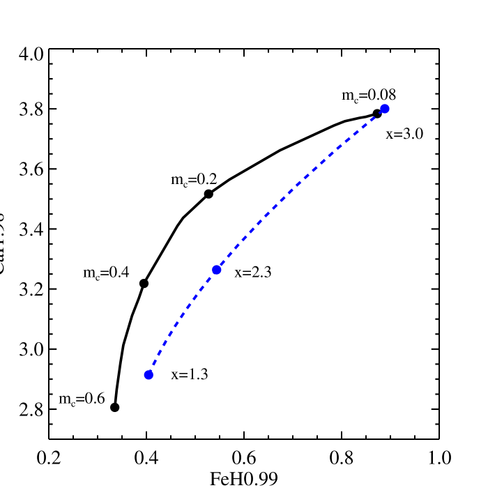
Figure 18.— Index-index diagram demonstrating that the combination of multiple IMF-sensitive indices can constrain the shape of the low-mass IMF. The CaI0.98 index is most sensitive to $M\approx 0.5M_{\odot}$ while the FeH0.99 index is most sensitive to $M<0.3M_{\odot}$ (see Figure 17). The figure shows models at solar metallicity with an age of 13.5 Gyr. One model track is shown for a power-law IMF with index $x$ that varies between $1.3<x<3.0$ for a fixed low-mass cutoff, $m_{c}=0.08M_{\odot}$. The second model track is shown for a fixed power-law index of $x=3.0$ and varying low-mass cutoff: $0.08M_{\odot}<m_{c}<0.6M_{\odot}$.

What is less obvious from this figure is how the detailed spectral shape around these features changes as the velocity dispersion is increased. Most notable is the fact that the NaI0.82 feature is resolved as a doublet at low dispersion, but is blended into a single feature at $\sigma>200\ {\rm km\,s}^{-1}$. This is an example where spectral indices neglect important details. In low dispersion systems, consideration of the full spectrum around the NaI doublet at 0.82$\mu m$ would provide much stronger constraints than mere consideration of the NaI0.82 index (see Figure 8; also Boroson & Thompson, 1991; Schiavon et al., 2000).

In Figures 12, 13, and 14 we have included error bars for $S/N=200$ Å^-1 spectra. These error bars demonstrate that a spectrum with this $S/N$ is sufficient to strongly differentiate between a Chabrier and Salpeter IMF in all of the IMF-sensitive indices. More generally, the $S/N$ per angstrom required to differentiate between a Chabrier and $x=3$ IMF at the $2\sigma$ level is 11, 29, 32, and 41 for the CO2.30, NaI0.82, FeH0.99, and CaII0.86 indices. In order to differentiate between a Chabrier and Salpeter IMF at the same level of significance, the required $S/N$ for the four indices is more demanding: 32, 105, 105 and 130.

It is difficult to make general comments regarding the level of flux calibration and sky subtraction necessary to measure the IMF, so we limit the following discussion to some simple statements. Absolute flux calibration is unnecessary for the measurement of narrow spectral features. Moreover, relative flux calibration is only necessary over $\sim 100$Å  wavelength intervals, owing to the necessity of sampling not only the feature of interest but some continuum blueward and redward of the feature (see Table 1). We have experimented with multiplying the model spectra by polynomials in order to assess the required level of relative flux calibration. Broadly speaking, polynomials with 10% amplitude variation over $\sim 100$Å  intervals result in $1-10$% changes to the indices. Of course, pathological polynomials, where a feature in the polynomial coincides with the feature of interest, result in much stronger changes to the indices. When strong sky lines coincide with a feature of interest it will be very difficult, if not impossible, to reach the required $S/N$ in the reduced spectrum. Stacking spectra with different redshifts in the restframe limits (or even eliminates) the influence of sky emission and absorption (see $\S$3, and e.g., van Dokkum & Conroy, 2010, 2011).

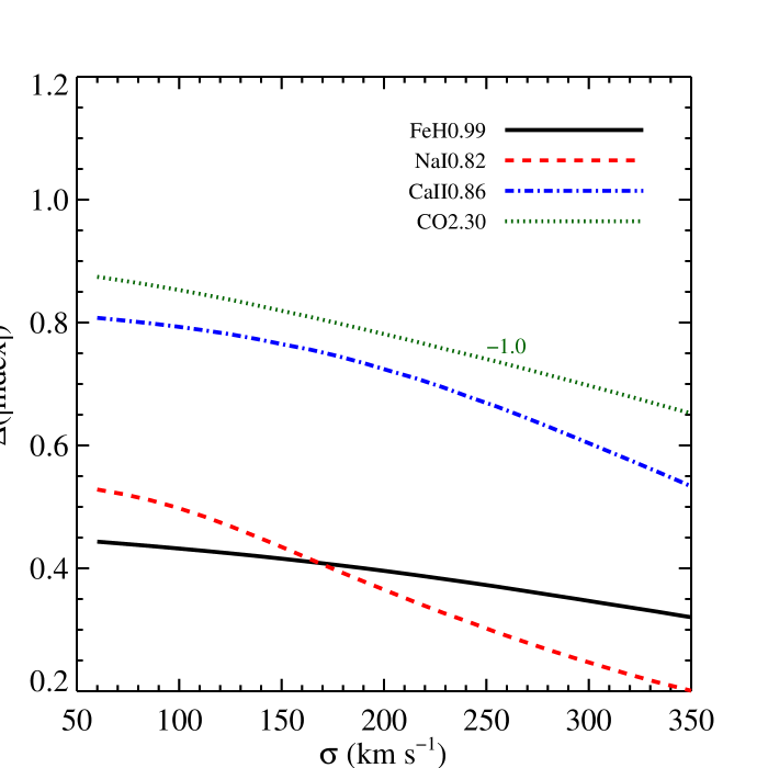
Figure 19.— Absolute change in selected indices between a Chabrier and $x=3$ IMF as a function of velocity dispersion. Indices are measured in EW with units of Å. The CO2.30 index has been shifted downward by 1Å  for clarity.

5. Discussion

5.1. What can be measured from integrated light

Our primary goal has been to investigate the extent to which the low-mass IMF can be directly constrained from integrated light spectra. We have demonstrated that the effect of the IMF on the red and near-IR spectra of old stellar populations is subtle but measurable and the effect becomes quite strong for IMFs steeper than the disk of the Galaxy. The only limitation of our approach is that the stellar population must be dominated by old ($\gtrsim 5$ Gyr) stars. Younger stars outshine the faint low mass stars by many orders of magnitude, rendering low-mass IMF measurements impossible. In addition, different spectral features respond to changes in the IMF in different ways, suggesting that the shape of the low-mass IMF can also be directly constrained from moderate resolution ($R\approx 2000$) spectra of distant galaxies. Based on the results shown in $\S$4.4 we expect that the shape of the IMF can be constrained in distant galaxies to at least $0.2M_{\odot}$. We have presented many of the key results of this paper using spectral indices. We emphasize that this was merely for clarity — when actually fitting models to data we advocate using the spectra directly for the reasons highlighted throughout this paper.

These results signal an important shift in stellar population studies. With the models presented in this paper we should be able to, for the first time, directly measure the IMF in distant galaxies, which means that we will be able to directly measure their total stellar mass (not including remnants). This measurement should be possible, in principle, out to redshifts of order unity for old stellar populations. At higher redshifts the age of the Universe sets an upper limit to the age of stellar systems that is younger than the applicability of this technique (e.g., $\gtrsim 5$ Gyr).

We have also demonstrated that the effect of the IMF in integrated light can be separated from elemental abundance effects. A powerful approach is to combine blue and red spectra because the faint M dwarfs of interest contribute approximately ten times less flux in the blue compared to the red. The blue spectrum is therefore much less IMF-sensitive than the red. Combining IMF-sensitive spectral features in the red with IMF-insensitive blue features dominated by the same element (e.g., FeI0.52 and FeH0.99) is the most promising means to separate IMF and abundance effects (see also Vazdekis et al., 2003; Cenarro et al., 2004, who make a similar point). The weak IMF-dependence in the blue spectral features, especially in the Lick-based indices explored in this work, suggests that previous work on constraining the mean stellar age and abundance patterns — based almost exclusively on blue spectra and indices — are relatively robust against changes to the IMF.

We highlight the Wing-Ford band, denoted herein as FeH0.99, as the most promising single feature for constraining the low-mass IMF. It is insensitive to age for ages $>5$ Gyr and insensitive to $\alpha-$enhancement. It depends on the iron abundance, which can be measured accurately and independently in the blue. It also depends only weakly on velocity dispersion because it is intrinsically broad. It is therefore an ideal indicator of the dwarf-to-giant ratio in old stellar populations.

All of the model results in this paper make the implicit assumption that the IMF is fully populated. This assumption is valid for systems with minimum masses in excess of $10^{5-6}M_{\odot}$, depending on wavelength and age (Lançon & Mouhcine, 2000; Cerviño & Luridiana, 2004; Popescu & Hanson, 2010). For galaxies and massive globular clusters, our assumption is therefore valid, while for less massive systems stochastic effects will need to be modeled.

5.2. Previous work

It has been known since at least the work of Spinrad (1962) that one could in principle measure the contribution of faint M dwarfs to the integrated light of old stellar populations. As noted in the introduction, previous observational work suffered from a number of technical obstacles including poor detector technology. Poor spectral resolution was also a problem. In an important early paper, Carter et al. (1986) attempted to measure the strength of the NaI0.82 feature in massive ellipticals, but they could not separate the NaI feature from the adjacent TiO feature, which is strong in giants, greatly complicating the interpretation (see also Delisle & Hardy, 1992). This is no longer a limitation with current instruments.

It is also worth noting that the scope of the discussion has changed markedly since the early papers of Spinrad & Taylor (1971), Cohen (1979), and Faber & French (1980). In that early work the question was whether or not M dwarfs dominated, or at least contributed significantly, to the integrated light. Spinrad & Taylor (1971) claimed, for example, that dwarfs contributed $\sim 30$% to the $V-$band light of old populations. This would imply a mass-to-light ratio of $M/L\approx 40$, which we know now is strongly ruled out on dynamical grounds (e.g., Cappellari et al., 2006). It is now generally agreed that dwarfs do not contribute substantially to the integrated light. The debate today centers on whether dwarfs contribute $\lesssim 1$% or several percent to the integrated light. This difference is quite subtle but of fundamental importance not only for questions regarding the universality of the IMF but also the relative amount of dark and luminous matter in the centers of galaxies.

Early models attempted to construct integrated light spectra from empirical stellar spectra (e.g., Carter et al., 1986). Among the limitations was again the quality of the data, and also the fact that the stellar libraries contained few M dwarfs. Schiavon et al. (2000) were the first to create fully synthetic population synthesis predictions in the near-IR with the aim of investigating the effects of the IMF, population age, and metallicity on the NaI, CaII, and FeH features. The state of population synthesis modeling has not changed qualitatively in the intervening decade. The most important improvements between this paper and Schiavon et al. (2000) are 1) the more comprehensive analysis of the blue through near-IR spectra as a function of IMF, age, and individual elemental abundances, 2) the use of empirical spectral libraries for the fiducial models, with the synthetic models being used only differentially, and 3) important updates to the model atmosphere and spectra calculations, including the addition of the H₂O linelist and improvements in other existing linelists such as TiO and FeH.

More recently, Cenarro et al. (2003) concluded that the IMF varies with velocity dispersion and [Fe/H] based on analysis of the CaII triplet, TiO, and MgI lines. That work lacked models with variable abundance ratios, and so the authors could not reliably separate IMF effects from abundance effects. Indeed, interpretation of calcium line strengths have led to many contradictory claims over the years, without a clear resolution (Thomas et al., 2003a; Falcón-Barroso et al., 2003; Cenarro et al., 2004; Worthey et al., 2011). The new models presented in the present work should be able to resolve the calcium puzzle.

5.3. van Dokkum & Conroy (2010)

In van Dokkum & Conroy (2010) we used the NaI0.82 and FeH0.99 spectral features to probe the low-mass IMF in eight massive ellipticals. Based on high signal-to-noise, $R\sim 2000$ spectra taken with the Keck telescope, we concluded that these galaxies had on average a much more bottom-heavy IMF compared to the Galaxy; an IMF between Salpeter and $x=3$ was preferred, although a quantitative assessment was not provided in that work. With the model results presented in this paper we are now in a position to reassess those conclusions.

The result of a bottom-heavy IMF in massive ellipticals was based on a preliminary version of the population synthesis model presented herein. In particular, the base isochrones and empirical IRTF spectra are essentially identical between that work and the present paper. The primary uncertainty in our previous work was the uncertain impact of elemental abundance variations and stellar population age effects on the NaI0.82 and FeH0.99 indices. This concern was particularly acute since it is known that the galaxies we targeted show $\alpha-$enhanced abundance patterns (in subsequent work we compared these massive elliptical spectra to metal-rich globular clusters in M31 that have similar abundance patterns and again found evidence for a bottom-heavy IMF in the ellipticals; see van Dokkum & Conroy, 2011, for details). In fact, one of the motivations for the present work was to assess the effect of abundance variations on our previous results.

In light of these concerns, the most important results from the present work are that the FeH0.99 index is essentially insensitive to [$\alpha$/Fe] and the NaI0.82 index is anti-correlated with [$\alpha$/Fe]. Thus, the construction of models more applicable to massive ellipticals, where [$\alpha$/Fe]$\sim 0.2$ and [Fe/H]$\sim 0.0$, will produce FeH0.99 and NaI0.82 strengths that still demand a bottom-heavy IMF in our sample of massive ellipticals. In order to explain the strengths of these features as being due to abundance effects would require an average iron abundance in excess of solar ([Fe/H]$\sim 0.15$) and an extremely high average sodium abundance ([Na/Fe]$>0.5$). The former would result in strong disagreement with the blue FeI lines. The latter is not directly constrained for massive ellipticals, but we note that in the bulge of the Galaxy, which is $\alpha-$enhanced like the massive ellipticals, [Na/Fe] is never greater than 0.3 dex and has an average of [Na/Fe]=0.2 (Fulbright et al., 2007). The only stars known to have very high sodium abundances ([Na/Fe]¿0.5) are found exclusively within globular clusters (Gratton et al., 2004).

Beyond confirming the somewhat qualitative analysis in our previous work, we aim to quantify the shape of the IMF and better constrain the number of low mass stars in massive elliptical galaxies. This requires a quantitative analysis of the blue and red spectra of our sample of massive ellipticals based on the models presented in this paper and is the subject of ongoing work.

5.4. On the fingerprints of M dwarfs in integrated light

The fundamental idea underpinning this paper is the fact that certain spectral features betray the presence of faint M dwarfs in integrated light spectra. This idea is based partly on the fact that certain spectral features depend strongly on surface gravity at fixed effective temperature. Although this fact is well known both empirically and via inspection of model spectra, we have been surprised by the lack of discussion in the literature regarding its physical origin. We have therefore endeavored to understand these surface gravity trends. What follows is a brief sketch of the basic physics involved; a more quantitative investigation is left for future work.

Careful inspection of Figure 10 reveals that every atomic feature that is strong in dwarfs is a neutral metal (e.g., NaI, KI, CaI, AlI), while every atomic feature that is strong in giants is a singly-ionized metal (specifically, CaII). This is a simple consequence of ionization equilibrium (i.e., the Saha equation): as the electron pressure increases at fixed temperature (due to the increased surface gravity), the ratio of singly-ionized to neutral species of the same atom decreases. We have confirmed this directly with the model atmospheres: for stars with $\ T_{\rm eff}=3500$ K, dwarfs have a higher relative abundance of NaI and a lower relative abundance of CaII compared to the giants.

The situation with molecules is similar to that of the atoms. Molecular dissociation equilibrium (Russell, 1934; Tsuji, 1973) implies that an increase in the partial pressures of the atoms and molecules favors the side of a given chemical reaction that results in fewer moles of gas. For example, the formation of H₂O is favored because its formation results in fewer moles of gas compared to its atomic constituents. This is also confirmed upon inspection of the model atmospheres: at a fixed effective temperature, molecules are in greater abundance with respect to hydrogen for the dwarfs compared to the giants.

An important exception to this rule is CO. It has the highest dissociation energy of any known molecule and therefore its formation is highly favored over other molecules that might compete for free carbon and oxygen. Its formation is so favored, in fact, that in the atmospheres of cool giants essentially all the carbon is locked in CO. This is important because it means that as the pressure is increased moving from a giant to a dwarf, the relative abundance of CO does not increase in the manner outlined above; all the carbon is already locked up in the most tightly bound molecule. This probably explains why CO features behave differentially from other features dominated by molecules.

Of course, consideration of the abundances of atoms and molecules is not sufficient to determine the qualitative behavior of spectral features. The strength of any spectral line is determined by the ratio of line opacity to continuum opacity. For example, the abundance of TiO is higher in dwarfs than in giants, indicating a higher line opacity, but the strength of TiO features is frequently much stronger in giants than in dwarfs. The difference must be due to the variation in the continuum opacity between dwarfs and giants. The situation is especially complex for M stars, as the near-IR continuum is largely determined by the H₂O opacity. Consideration of these effects is beyond the scope of the present paper. The basic point we wish to make here is that it should not be surprising that the neutral metals generically behave oppositely to the singly-ionized metals, and that CO should behave differently from all other molecules in late-type stars.

For certain features there is yet another factor determining their sensitivity to M dwarfs. From the isochrones shown in Figure 1 it is clear that the faintest M dwarfs are substantially cooler than the faintest M giants for an age of 13.5 Gyr (2000 K vs. 3000 K). It is also evident from Figure 7 that features such as NaI0.82, FeH0.99, and KI1.17 become much stronger at $\ T_{\rm eff}<3000$ K. This is an important point because it means that at least some IMF-sensitive features are IMF-sensitive both because they are sensitive to surface gravity and because they vary strongly with effective temperature amongst late-type stars.

6. Summary

We now summarize our main conclusions.

• Low-mass stars impart a unique signature on the integrated spectrum of old stellar populations. Spectral features sensitive to low-mass stars reside in the red and near-IR and arise from lines of various elements and molecules (including Ca, Na, K, Al, CO, and FeH). The low-mass IMF can therefore be inferred directly from red/near-IR spectra of old populations despite the fact that low-mass stars comprise only a few percent of the bolometric luminosity.

• These IMF-sensitive features also vary with elemental abundance patterns and some vary with stellar age. Fortunately, the combination of IMF-sensitive features in the red with IMF-insensitive features in the blue provides a joint constraint on the IMF, stellar age, metallicity, and abundance pattern. The FeH feature at 0.99$\mu m$ is particularly promising because it is insensitive to $\alpha$-enhancement and stellar ages of $5-13.5$ Gyr. The triplet of CaII features near 0.86$\mu m$ are also promising if considered in conjunction the CaI doublet at 1.98$\mu m$ since these features respond strongly and with opposite sign to variations in the IMF.

• It is difficult to mimic IMF effects with other exotic modifications to standard population synthesis, such as an arbitrary increase or decrease in the number of RGB, HB, and/or AGB stars. The strength of the TiO band-head at 0.89$\mu m$ provides a strong constraint on the contribution of very late M giants to the integrated spectrum.

• Each of the IMF-sensitive features explored in this work is sensitive to a different regime of the low-mass IMF. It should therefore be possible to directly constrain the shape of the low-mass IMF from integrated spectra of old stellar populations.

It has been appreciated for several decades that it is possible to constrain the mean stellar age, metallicity, and abundances of at least some elements from the integrated light spectrum of old stellar populations. The models presented in this work demonstrate that the low-mass IMF should be added to this list of physical properties to be constrained directly by the data.

The models presented in this paper will be made available upon request.

References

- Alonso et al. (1996) Alonso, A., Arribas, S., & Martinez-Roger, C. 1996, A&A, 313, 873
- Alonso et al. (1999) Alonso, A., Arribas, S., & Martínez-Roger, C. 1999, A&AS, 140, 261
- An et al. (2009) An, D. et al. 2009, ApJ, 700, 523
- Anders & Grevesse (1989) Anders, E. & Grevesse, N. 1989, Geochim. Cosmochim. Acta, 53, 197
- Asplund et al. (2009) Asplund, M., Grevesse, N., Sauval, A. J., & Scott, P. 2009, ARA&A, 47, 481
- Baraffe et al. (1998) Baraffe, I., Chabrier, G., Allard, F., & Hauschildt, P. H. 1998, A&A, 337, 403
- Boroson & Thompson (1991) Boroson, T. A. & Thompson, I. B. 1991, AJ, 101, 111
- Bruzual & Charlot (2003) Bruzual, G. & Charlot, S. 2003, MNRAS, 344, 1000
- Burstein et al. (1984) Burstein, D., Faber, S. M., Gaskell, C. M., & Krumm, N. 1984, ApJ, 287, 586
- Caldwell et al. (2011) Caldwell, N., Schiavon, R., Morrison, H., Rose, J. A., & Harding, P. 2011, AJ, 141, 61
- Cappellari et al. (2006) Cappellari, M. et al. 2006, MNRAS, 366, 1126
- Carter et al. (1986) Carter, D., Visvanathan, N., & Pickles, A. J. 1986, ApJ, 311, 637
- Casagrande et al. (2008) Casagrande, L., Flynn, C., & Bessell, M. 2008, MNRAS, 389, 585
- Casagrande et al. (2010) Casagrande, L., Ramírez, I., Meléndez, J., Bessell, M., & Asplund, M. 2010, A&A, 512, A54
- Cenarro et al. (2001) Cenarro, A. J., Cardiel, N., Gorgas, J., Peletier, R. F., Vazdekis, A., & Prada, F. 2001, MNRAS, 326, 959
- Cenarro et al. (2009) Cenarro, A. J., Cardiel, N., Vazdekis, A., & Gorgas, J. 2009, MNRAS, 396, 1895
- Cenarro et al. (2003) Cenarro, A. J., Gorgas, J., Vazdekis, A., Cardiel, N., & Peletier, R. F. 2003, MNRAS, 339, L12
- Cenarro et al. (2004) Cenarro, A. J., Sánchez-Blázquez, P., Cardiel, N., & Gorgas, J. 2004, ApJ, 614, L101
- Cenarro et al. (2007) Cenarro, A. J. et al. 2007, MNRAS, 374, 664
- Cerviño & Luridiana (2004) Cerviño, M. & Luridiana, V. 2004, A&A, 413, 145
- Chabrier (2003) Chabrier, G. 2003, PASP, 115, 763
- Chabrier & Baraffe (1997) Chabrier, G. & Baraffe, I. 1997, A&A, 327, 1039
- Coelho et al. (2007) Coelho, P., Bruzual, G., Charlot, S., Weiss, A., Barbuy, B., & Ferguson, J. W. 2007, MNRAS, 382, 498
- Cohen (1978) Cohen, J. G. 1978, ApJ, 221, 788
- Cohen (1979) —. 1979, ApJ, 228, 405
- Conroy et al. (2009) Conroy, C., Gunn, J. E., & White, M. 2009, ApJ, 699, 486
- Couture & Hardy (1993) Couture, J. & Hardy, E. 1993, ApJ, 406, 142
- Cushing et al. (2005) Cushing, M. C., Rayner, J. T., & Vacca, W. D. 2005, ApJ, 623, 1115
- Delfosse et al. (2000) Delfosse, X., Forveille, T., Ségransan, D., Beuzit, J.-L., Udry, S., Perrier, C., & Mayor, M. 2000, A&A, 364, 217
- Delisle & Hardy (1992) Delisle, S. & Hardy, E. 1992, AJ, 103, 711
- Diaz et al. (1989) Diaz, A. I., Terlevich, E., & Terlevich, R. 1989, MNRAS, 239, 325
- Dotter et al. (2007) Dotter, A., Chaboyer, B., Ferguson, J. W., Lee, H.-c., Worthey, G., Jevremović, D., & Baron, E. 2007, ApJ, 666, 403
- Dotter et al. (2008) Dotter, A., Chaboyer, B., Jevremović, D., Kostov, V., Baron, E., & Ferguson, J. W. 2008, ApJS, 178, 89
- Dulick et al. (2003) Dulick, M., Bauschlicher, Jr., C. W., Burrows, A., Sharp, C. M., Ram, R. S., & Bernath, P. 2003, ApJ, 594, 651
- Faber & French (1980) Faber, S. M. & French, H. B. 1980, ApJ, 235, 405
- Falcón-Barroso et al. (2003) Falcón-Barroso, J., Peletier, R. F., Vazdekis, A., & Balcells, M. 2003, ApJ, 588, L17
- Falcón-Barroso et al. (2011) Falcón-Barroso, J., Sánchez-Blázquez, P., Vazdekis, A., Ricciardelli, E., Cardiel, N., Cenarro, A. J., Gorgas, J., & Peletier, R. F. 2011, A&A, 532, A95
- Frogel et al. (1980) Frogel, J. A., Persson, S. E., & Cohen, J. G. 1980, ApJ, 240, 785
- Frogel et al. (1978) Frogel, J. A., Persson, S. E., Matthews, K., & Aaronson, M. 1978, ApJ, 220, 75
- Frogel & Whitford (1987) Frogel, J. A. & Whitford, A. E. 1987, ApJ, 320, 199
- Fulbright et al. (2007) Fulbright, J. P., McWilliam, A., & Rich, R. M. 2007, ApJ, 661, 1152
- Gratton et al. (2004) Gratton, R., Sneden, C., & Carretta, E. 2004, ARA&A, 42, 385
- Grevesse & Sauval (1998) Grevesse, N. & Sauval, A. J. 1998, Space Sci. Rev., 85, 161
- Hardy & Couture (1988) Hardy, E. & Couture, J. 1988, ApJ, 325, L29
- Ivanov et al. (2004) Ivanov, V. D., Rieke, M. J., Engelbracht, C. W., Alonso-Herrero, A., Rieke, G. H., & Luhman, K. L. 2004, ApJS, 151, 387
- Jensen et al. (2003) Jensen, J. B. et al. 2003, ApJ, 583, 712
- Kleinmann & Hall (1986) Kleinmann, S. G. & Hall, D. N. B. 1986, ApJS, 62, 501
- Korn et al. (2005) Korn, A. J., Maraston, C., & Thomas, D. 2005, A&A, 438, 685
- Kroupa (2001) Kroupa, P. 2001, MNRAS, 322, 231
- Kurucz (1970) Kurucz, R. L. 1970, SAO Special Report, 309
- Kurucz (1993) —. 1993, SYNTHE spectrum synthesis programs and line data, ed. Kurucz, R. L.
- Kurucz & Avrett (1981) Kurucz, R. L. & Avrett, E. H. 1981, SAO Special Report, 391
- Lançon & Mouhcine (2000) Lançon, A. & Mouhcine, M. 2000, in Astronomical Society of the Pacific Conference Series, Vol. 211, Massive Stellar Clusters, ed. A. Lançon & C. M. Boily, 34
- Lee et al. (2009) Lee, H.-c., Worthey, G., Dotter, A., Chaboyer, B., Jevremović, D., Baron, E., Briley, M. M., Ferguson, J. W., Coelho, P., & Trager, S. C. 2009, ApJ, 694, 902
- Liu et al. (2002) Liu, M. C., Graham, J. R., & Charlot, S. 2002, ApJ, 564, 216
- Marigo et al. (2008) Marigo, P., Girardi, L., Bressan, A., Groenewegen, M. A. T., Silva, L., & Granato, G. L. 2008, A&A, 482, 883
- Mármol-Queraltó et al. (2008) Mármol-Queraltó, E., Cardiel, N., Cenarro, A. J., Vazdekis, A., Gorgas, J., Pedraz, S., Peletier, R. F., & Sánchez-Blázquez, P. 2008, A&A, 489, 885
- Partridge & Schwenke (1997) Partridge, H. & Schwenke, D. W. 1997, Journal of Chemical Physics, 106, 4618
- Perrin et al. (1998) Perrin, G., Coudé du Foresto, V., Ridgway, S. T., Mariotti, J.-M., Traub, W. A., Carleton, N. P., & Lacasse, M. G. 1998, A&A, 331, 619
- Popescu & Hanson (2010) Popescu, B. & Hanson, M. M. 2010, ApJ, 713, L21
- Prugniel & Soubiran (2001) Prugniel, P. & Soubiran, C. 2001, A&A, 369, 1048
- Ramírez & Meléndez (2005) Ramírez, I. & Meléndez, J. 2005, ApJ, 626, 465
- Rayner et al. (2009) Rayner, J. T., Cushing, M. C., & Vacca, W. D. 2009, ApJS, 185, 289
- Renzini & Voli (1981) Renzini, A. & Voli, M. 1981, A&A, 94, 175
- Ridgway et al. (1980) Ridgway, S. T., Joyce, R. R., White, N. M., & Wing, R. F. 1980, ApJ, 235, 126
- Russell (1934) Russell, H. N. 1934, ApJ, 79, 317
- Sánchez-Blázquez et al. (2006) Sánchez-Blázquez, P., Peletier, R. F., Jiménez-Vicente, J., Cardiel, N., Cenarro, A. J., Falcón-Barroso, J., Gorgas, J., Selam, S., & Vazdekis, A. 2006, MNRAS, 371, 703
- Sbordone et al. (2004) Sbordone, L., Bonifacio, P., Castelli, F., & Kurucz, R. L. 2004, Memorie della Societa Astronomica Italiana Supplementi, 5, 93
- Schiavon (2007) Schiavon, R. P. 2007, ApJS, 171, 146
- Schiavon et al. (2000) Schiavon, R. P., Barbuy, B., & Bruzual A., G. 2000, ApJ, 532, 453
- Schiavon et al. (1997a) Schiavon, R. P., Barbuy, B., Rossi, S. C. F., & Milone, A. 1997a, ApJ, 479, 902
- Schiavon et al. (1997b) Schiavon, R. P., Barbuy, B., & Singh, P. D. 1997b, ApJ, 484, 499
- Schiavon et al. (2004) Schiavon, R. P., Caldwell, N., & Rose, J. A. 2004, AJ, 127, 1513
- Schwenke (1998) Schwenke, D. W. 1998, Faraday Discussions, 109, 321
- Serven et al. (2005) Serven, J., Worthey, G., & Briley, M. M. 2005, ApJ, 627, 754
- Spinrad (1962) Spinrad, H. 1962, ApJ, 135, 715
- Spinrad & Taylor (1971) Spinrad, H. & Taylor, B. J. 1971, ApJS, 22, 445
- Strader et al. (2011) Strader, J., Caldwell, N., & Seth, A. C. 2011, AJ, 142, 8
- Thomas et al. (2003a) Thomas, D., Maraston, C., & Bender, R. 2003a, MNRAS, 343, 279
- Thomas et al. (2003b) —. 2003b, MNRAS, 339, 897
- Thomas et al. (2005) Thomas, D., Maraston, C., Bender, R., & Mendes de Oliveira, C. 2005, ApJ, 621, 673
- Tonry et al. (2001) Tonry, J. L. et al. 2001, ApJ, 546, 681
- Trager et al. (2000) Trager, S. C., Faber, S. M., Worthey, G., & González, J. J. 2000, AJ, 120, 165
- Trager et al. (1998) Trager, S. C., Worthey, G., Faber, S. M., Burstein, D., & Gonzalez, J. J. 1998, ApJS, 116, 1
- Tripicco & Bell (1995) Tripicco, M. J. & Bell, R. A. 1995, AJ, 110, 3035
- Tsuji (1973) Tsuji, T. 1973, A&A, 23, 411
- Valdes et al. (2004) Valdes, F., Gupta, R., Rose, J. A., Singh, H. P., & Bell, D. J. 2004, ApJS, 152, 251
- Valenti & Fischer (2005) Valenti, J. A. & Fischer, D. A. 2005, ApJS, 159, 141
- van Dokkum (2008) van Dokkum, P. G. 2008, ApJ, 674, 29
- van Dokkum & Conroy (2010) van Dokkum, P. G. & Conroy, C. 2010, Nature, 468, 940
- van Dokkum & Conroy (2011) —. 2011, ApJ, 735, L13
- Vazdekis et al. (1996) Vazdekis, A., Casuso, E., Peletier, R. F., & Beckman, J. E. 1996, ApJS, 106, 307
- Vazdekis et al. (2003) Vazdekis, A., Cenarro, A. J., Gorgas, J., Cardiel, N., & Peletier, R. F. 2003, MNRAS, 340, 1317
- Vazdekis et al. (2010) Vazdekis, A., Sánchez-Blázquez, P., Falcón-Barroso, J., Cenarro, A. J., Beasley, M. A., Cardiel, N., Gorgas, J., & Peletier, R. F. 2010, MNRAS, 404, 1639
- Walcher et al. (2009) Walcher, C. J., Coelho, P., Gallazzi, A., & Charlot, S. 2009, MNRAS, 398, L44
- West et al. (2004) West, A. A. et al. 2004, AJ, 128, 426
- Wing & Ford (1969) Wing, R. F. & Ford, Jr., W. K. 1969, PASP, 81, 527
- Worthey et al. (1992) Worthey, G., Faber, S. M., & Gonzalez, J. J. 1992, ApJ, 398, 69
- Worthey et al. (1994) Worthey, G., Faber, S. M., Gonzalez, J. J., & Burstein, D. 1994, ApJS, 94, 687
- Worthey et al. (2011) Worthey, G., Ingermann, B. A., & Serven, J. 2011, ApJ, 729, 148
- Wu et al. (2011) Wu, Y., Singh, H. P., Prugniel, P., Gupta, R., & Koleva, M. 2011, A&A, 525, A71