Search for z$\sim$6.96 Ly$\alpha$ emitters with Magellan/IMACS in the COSMOS field

Abstract

We report a search for z$\sim$6.96 Ly$\alpha$ emitters (LAEs) using a Narrow-Band filter, centered at 9680Å  with the IMACS instrument on the Magellan telescope at Las Campanas Observatory. We obtain a sample of 6 Ly$\alpha$ emitter candidates of luminosity $\sim 10^{42}\mathrm{erg}\,\mathrm{s}^{-1}$ in a total area of 465 square arcmin corresponding to a comoving volume of $\sim 72000Mpc^{3}$.
From this result, we derive a Ly$\alpha$ luminosity function (LF) at z$\sim$6.96 and compare our sample with the only z$\sim$6.96 Ly$\alpha$ emitter spectroscopically confirmed to date (Iye et al., 2006). We find no evolution between the z=5.7 and z$\sim$7 Ly$\alpha$ luminosity functions, if a majority of our candidates are confirmed. Spectroscopic confirmation for this sample will enable more robust conclusions.

1 Introduction

Over the last decade, significant progress has been made in determining the processes of galaxy evolution using both ground- and space-based telescopes. Currently, the limits of the observable universe are at z $\sim 6$, which corresponds to $\sim 90\%$ the age of the universe. At z$>$6, we are approaching the NIR domain : the sky is brighter and it is more challenging to detect the faint high redshift sources. Beyond this boundary lie the first ultraviolet (UV)-emitting sources, which ionized the majority of the hydrogen in the universe. Their detection will allow us to probe the era of reionization, after the “Dark Ages”. Galaxies formed at high redshifts play a key role in understanding how and when the reionization of the universe took place. They also help constrain the physical mechanisms that drove the formation of the first stars and galaxies in the universe.

Starbursting galaxies can emit a large fraction of their ultraviolet luminosity in the Ly$\alpha$ line. Because Ly$\alpha$ photons are resonantly scattered in neutral hydrogen, even a small amount of dust can quench this emission. Hence, selecting objects with strong Ly$\alpha$ emission lines is expected to reveal a set of objects in the early phases of rapid star formation. These could either be young objects in their first burst of star formation or evolved galaxies undergoing a starburst due to a recent merger. Selecting galaxies with strong emission lines also allows us to probe the high-redshift Ly$\alpha$ luminosity function (LF).
Once the Ly$\alpha$ LF is determined, it is then possible to infer the ionization fraction of the intergalactic medium (IGM) at different redshifts (Malhotra & Rhoads, 2004; Stern et al., 2005; Furlanetto et al., 2006; Kashikawa et al., 2006; Ouchi et al., 2010). The presence of neutral hydrogen in the IGM can reduce the Ly$\alpha$ flux of galaxies, it is therefore clear that the Ly$\alpha$ LF is sensitive to the ionization fraction of the Universe. If we knew the intrinsic LF(z) of galaxies at each redshift, a deviation of the observed LF from this intrinsic distribution could be attributed to the attenuation by HI, and hence be used to infer the ionization fraction. In practice, the approach is to do proceed to a comparison of Ly$\alpha$ LF at different redshifts, since the LFs of Ly$\alpha$ emitters (LAEs) don’t evolve much between z=3-5.7 (Cassata et al., 2010; Malhotra et al., 2011).

With ground-based telescopes, the detection of very distant objects requires observation of UV spectral signatures that have been redshifted into the visible spectrum. The longer the wavelength of the observed Ly$\alpha$ line, the earlier the epoch at which we observe the galaxy, and the closer to the “Dark Ages”. Therefore, one way of searching for the most distant galaxies is to search for the redshifted Ly$\alpha$ emission at the longest possible wavelength. However, this search is complicated by the presence of OH emission lines within the terrestrial atmosphere, at an altitude of $\approx 80km$. This strong line emission limits the sensitivity of ground-based telescopes at near-infrared wavelengths. Fortunately, there are spectral intervals with lower OH-background that allow for a fainter detection limit from the ground.

We use a custom-built filter, $NB9680$, centered at $\lambda=9680\AA\$ and with a width of 90Åto use one of the low-sky windows. Narrow-band imaging is the most successful method to detect strong Ly$\alpha$ emission lines of galaxies, since it relies on a specific redshift interval as well as a selected low-sky background window. Adapting the spectral width of this filter allows for maximum detection of light from the celestial objects at that spectral line, while minimizing the adverse influences of sky emission.

The first $z>6$ LAEs was detected with the narrow-band (NB) technique at the 10m KeckII telescope (Hu et al., 2002). This galaxy was spectroscopically confirmed to be at $z=6.56$. Over $1,000$ LAEs have been photometrically selected and spectroscopically identified in this way. Extensive observations have been done at redshifts 5.7 and 6.5, two spectral domains free of sky lines in the optical spectrum, and different conclusions on the Luminosity Function are discussed by several groups (Malhotra & Rhoads, 2004, 2006; Ouchi et al., 2008; Cassata et al., 2010; Ouchi et al., 2008; Ota et al., 2008; Iye et al., 2006; Kashikawa et al., 2006; Shimasaku et al., 2006). Several surveys have attempted to observe z$\sim$7.7 (Hibon et al., 2010; Tilvi et al., 2010) and z$\sim$8.8 (Cuby et al., 2007; Willis et al., 2008), with no spectroscopic confirmation yet.
We present here a new NB imaging survey with the IMACS/Magellan telescope – targeting $z=6.96$ LAEs. This paper first presents the data (Section 2.1) and the data reduction procedure (Section 2.2). We then describe the method of selection and contamination of low-redshift interlopers for high redshift LAEs in Section 3. We present the final sample of $z=6.96$ LAEs and Ly$\alpha$ luminosity function at this redshift in Section 4.

Throughout this study, we adopt the following cosmological parameters : $H_{0}=70km.s^{-1}.Mpc^{-1}$, $\Omega_{m}=0.3$, $\Omega_{\Lambda}=0.7$ (Spergel et al., 2007). All magnitudes are AB magnitudes.

2 Observations and Data Reduction

2.1 Observations

The data were taken with the IMACS instrument (the Inamori-Magellan Area Camera & Spectrograph), installed at the 6.5m Magellan Baade telescope at Las Campanas Observatory. This instrument offers two cameras: f/2 and f/4, with different imaging scales and dispersions. We observed with the f/2 camera which delivers an image of 27.4’ diameter field at a scale of 0.2 arcsec per pixel. To ensure background limited performance, each exposure lasted 15 min. After each exposure, the telescope was offset and a new exposure was taken. The offset values, for each exposure, was randomly chosen.
We targeted one COSMOS field (RA=10:00:29 Dec=02:12:21) covered by the Canada France Hawaii Telescope Legacy Survey (CFHTLS) and the WIRCam Deep Survey (WIRDS : PIs Willott & Kneib). The total area of the survey is 572 square arcminutes. We observed using the NB filter centered at 9680Å ($NB9680$) on the 17th, 18th and 19th March 2009. During these observations, the conditions were good : we obtained 19, 23, and 19 15-minute exposures during these nights, with a seeing varying between 0.45” and 0.8”.

We observed the field again on the 21st, 22nd and 23rd March 2010. Between the 2009 and 2010 observing season, the filter was replaced with a new one built to have identical bandpass specifications. There is no major difference between the two filters’ realized bandpass, and we treat data from the two identically. The night conditions were not as good as those in 2009 : the seeing varied from 0.7” to 1.3” and we lost on average 2 hours per night due to instrument problems. We obtained 16, 19, and 18 15-minute exposures in three nights. The total exposure time for each epoch of data is given in Table 1.

2.2 NB Data Reduction

2.2.1 Data reduction

To process this data, we use the package MSCRED/IRAF. At the beginning of each night, we take 10 bias frames and 10 dome flats, we process the bias frames by overscan subtraction, trimming, and stacking to produce a master bias frame for each night. The science frames are bias subtracted and flat field corrected in the standard way. But the main difficulty was the fringing correction.

We see fringes produced by the interference of light reflected between parallel surfaces in an instrument. All object frames do not always share the same fringe pattern because flexure and variations in illumination geometry can change its amplitude or period even on short timescales. In order to correct each individual image for fringes, we produce a median image per night. An illumination frame is also generated for each science frame using a two-stage median smoothing algorithm, applied on each frame with a first stage filtering on a 16 pixel scale, the second on a 24 pixel scale. The net effect is comparable to a 384 pixel median filter corresponding to 76.8 arcsec.

We then produce a median of the illumination frame for each night and correct the science frames for the illumination pattern. We subtract this illumination frame from the median of the science frame to obtain a fringe pattern for each night. It is then essential to find the optimal multiplicative scaling factor to use in removing the fringe pattern from each science frame, as we have long exposure frames and the fringe pattern changes with time. Once the frames are corrected for the fringes, we perform a sky subtraction by subtracting a normalized median image of all science frames from each frame. Finally, once the sky-subtracted frames are reconstructed as single extension images, we stack them using the mscstack/IRAF task. We made stacks per night, per epoch and a combined epoch stack.

Astrometric calibration. We perform the astrometric calibration on the individual images before the final stacking. We set an initial WCS information in the header of the frames based on the COSMOS catalog. We need then to adjust the WCS parameters to obtain a more precise alignment. For this purpose we use mscwcs to apply a first offset on the (RA,Dec) coordinates and we refine the calibration by checking the alignment with msccmatch task.We finally obtain an astrometry calibration for each individual images with a precision of rms$\sim\pm 0.1$ arcsec in both directions.

Photometric calibration. The photometric calibration of the CFHTLS data is based on the SDSS data for stars with 17$<$i’$<$21 and the Megacam-SDSS color transformation equations of Regnault et al. (2009).The precision obtained in $u^{\ast}$, $g^{\prime}$, $r^{\prime}$, $i^{\prime}$, $z^{\prime}$ is between 0.03 and 0.02 mag. As the $NB9680$ filter is included in the $z^{\prime}$-band filter, we used the MAG AUTO magnitude from the $z^{\prime}$ band SExtractor catalog to calibrate our $NB9680$ filter. We select 1048 non-saturated stars in the magnitude range 16$<z^{\prime}<$20 to perform the calibration. Considering the photometric error on the broad-band (BB) calibration, we obtain a photometric calibration precise to 0.1 magnitude in $NB9680$.

Completeness. We estimate the limiting magnitude for the different bands by adding 200 artificial star-like objects per bin of 0.1 magnitude in blank regions of the different stacked images. We then run SExtractor on the image with the same parameters as previously used for object detection. We repeat this procedure 40 times. The average count on 40 times of the number of artificial stars retrieved in each magnitude bin provides a direct measure of the completeness limit. We report the 50% completeness limit in Table 1.
We use this result to determine the Luminosity Function presented in Section 4.

2.3 Broad Band Data

The CFHT-LS provides extremely deep optical imaging data for our observed field. For the purpose of this study, we made use of the T0006 release. The CFHT-LS data products are available from the CADC archive to CFHT users and take form of image stacks in the $u^{\ast}$, $g^{\prime}$, $r^{\prime}$, $i^{\prime}$, $z^{\prime}$ filters and of ancillary data such as weight maps, catalogs etc. The spectral curves of the filter $u^{\ast}$, $g^{\prime}$, $r^{\prime}$, $i^{\prime}$, $z^{\prime}$ are similar to the ones of SDSS filters. In addition to the optical data, we also have the WIRDS survey, providing $J$, $H$, $Ks$.These optical data have been calibrated photometrically using the SDSS photometry and the NIR data using 2MASS photometry (McCracken et al., 2010). Considering internal and external photometric error sources, the uncertainty on the optical and the NIR data photometry is $\sim$0.05 mag and $\sim$0.02 mag, respectively.
As the broad-band data and the narrow-band data do not have the same pixel scale, we resample the broad-band data using the software SWARP to obtain optical and NIR images with 0.2 arcsec/pixel. The alignment in pixels is then verified using IRAF geomap/geotran tasks. Our complete set of data is therefore scaled at 0.2 arcsec/pixel and covers an area of 27.4’ diameter. A summary of the observational data used in this paper is provided in Table 1. Figure 1 shows the transmission curves of the filters corresponding to the multi-band data used in this study.

Table 1: Observational data.

Instrument	Band	Integration	Limiting
		time (hrs)	magnitudea
MegaCam	$u^{\ast}$	12.5	26.6
MegaCam	$g^{\prime}$	20.25	27.9
MegaCam	$r^{\prime}$	37.6	27.6
MegaCam	$i^{\prime}$	54	27.3
MegaCam	$z^{\prime}$	40.1	26.4
IMACS	$NB9680$ 1st epoch	15.25	25.
IMACS	$NB9680$ 2nd epoch	13.25	25.b
IMACS	$NB9680$ combined	28.3	25.2c
WIRCam	$J$		24.8
WIRCam	$H$		24.9
WIRCam	$K_{\mathrm{s}}$		25

• $5\sigma$ magnitude limits in apertures 1″ in diameter for MegaCam and WIRCam. These limits correspond to a 50% completeness level.

• The filter used during 2010 observations has a better transmitted wavefront than the filter used in 2009. This explains the similar limiting magnitude between the two epochs although the observing conditions were different.

• By combining the two epochs of data, we should have expected a sensitivity increase of 0.37 mag. But the limit has increased by only 0.2 mag. This could be due to a systematic noise component like the fringes.
  

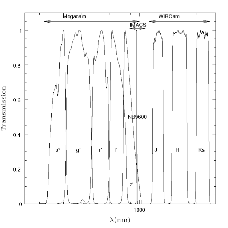
Figure 1: Transmission curves of the filters corresponding to the data used in this paper. All transmissions include the response of the detector and are normalized to 100% at maximum.

3 Sample

3.1 Catalog generation and Selection

We generate the catalogs using the software SExtractor (Bertin & Arnouts, 1996). We use the dual-image mode : the first image, for the detection, is settled as the combined $NB9680$ image, the second image, for measurement, corresponds to the resampled images from the optical and NIR bands. We choose to detect objects in 7 pixels above a threshold of 1.5$\sigma$, corresponding to a $NB9680\sim 25.8$. The aperture used for the photometry is 1 arcsec diameter.

As the IMACS instrument is composed of eight chips, we see an increase of the noise in the inter-chip regions. The sky noise is higher by a factor 2.5 in the interchip regions. We choose therefore to eliminate these regions from the area of the survey. From the total area covered by our survey, 572 square arcminutes, we obtain an effective area to search for z$\sim$6.96 LAE candidates of 465 square arcminutes.

Criterion#1 : Since we have two epochs of data, we define $NB9680$ selection criteria on individual epochs and on the combined images. We select objects with a 3$\sigma$ detection in both of the individual epoch images and a 5$\sigma$ detection in the combined $NB9680$ image. 59% (=16150 objects) of the objects present in the initial catalog pass this criterion. This eliminates variable sources from the catalog.

Criterion#2 : Due to the nearly complete absorption of the flux shortward of Ly$\alpha$ by the intergalactic Hydrogen, we should observe flux discontinuity at rest wavelength of 1216Å, and observed wavelength of 9680Å.We are therefore searching for objects which are not detectable in optical ($u^{\ast}$, $g^{\prime}$, $r^{\prime}$, $i^{\prime}$) bands. A possible method is therefore to select objects with less than a 3$\sigma$ detection in filters blueward of the expected Ly$\alpha$ emission : $u^{\ast}$, $g^{\prime}$, $r^{\prime}$, $i^{\prime}$.
We use a $\chi^{2}$ image generated by combining $g^{\prime}$, $r^{\prime}$ and $i^{\prime}$ CFHT data to obtain deep photometry of candidates in the combined optical bands. 3% of remaining candidates are accepted on this basis.

Criterion#3 : Following the successful method of Rhoads & Malhotra (2001) used for the search of z=5.7 LAEs in the LALA field, we require that more than 50% of the $NB9680$ flux comes from an emission line for object selection, which can be translated as $mag_{NB9680}-mag_{z^{\prime}}<-0.75mag$. This criterion is indicated in Figure 2, showing the $z^{\prime}-$$NB9680$ color versus $NB9680$ magnitude diagram. 88% of the objects selected after the criterion#2, pass this color restriction.

Criterion#4 : To avoid selecting extremely red objects (Cimatti et al., 2002), we choose to set a different criterion : $mag_{NB9680}-mag_{J}<0$. 98% of the objects selected after the criterion#3 pass this color criterion.

Criterion#5 : After applying carefully all the criteria presented above, we inspect each candidate visually. 33% of the objects inspected carefully are selected as serious candidates. the rest are rejected because they are near chip boundaries, or they are defects, etc.

The equations summarizing this selection are presented in the Table 2.

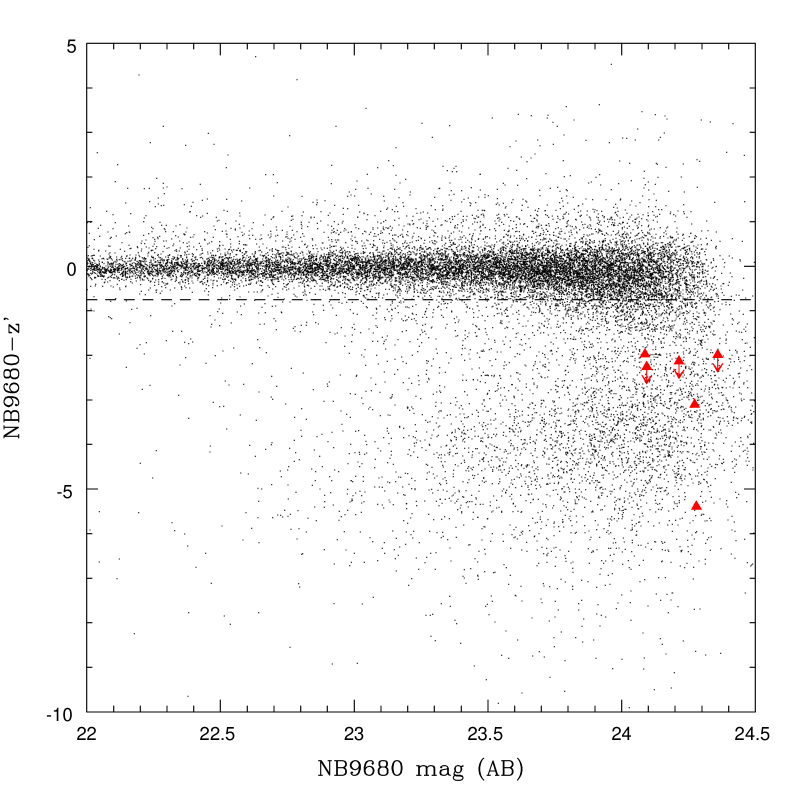
Figure 2: Color-Magnitude Diagram $z^{\prime}$-$NB9680$ vs $NB9680$ showing the candidates obtained with our criterion $mag_{NB9680}-mag_{z^{\prime}}<-0.75mag$ (plain red triangle). The other points with $mag_{NB9680}-mag_{z^{\prime}}<-0.75mag$ are ruled out by other criteria (blue flux, variability etc..).

Table 2: Table of the selection criteria.

	Our criteria
Criterion#1	SNR($NB9680_{combined}$)$>5\sigma$
	SNR($NB9680_{2009}$)$>3\sigma$
	SNR($NB9680_{2010}$)$>3\sigma$
Criterion#2	SNR($u^{\ast}$, $g^{\prime}$, $r^{\prime}$, $i^{\prime}$)$<3\sigma$
Criterion#3	$mag_{NB9680}-mag_{z^{\prime}}<-0.75mag$
Criterion#4	$mag_{NB9680}-mag_{J}<0$

3.2 Contaminants

COSMOS photometric redshift catalog gives us a first insight on the low redshift emitters contaminating our high redshift candidates sample.

Transient objects. Our strategy of observing the same field during two different years, and our requirement that the eligible candidates have to be detected in each epoch data within 3$\sigma$ level, allow us to rule out the contamination of our sample by transient objects such as supernovae, which would have appear in only one epoch of data. This strategy likewise prevents contamination by slow-moving solar system objects.

L-T dwarfs stars. Following the method described in Hibon et al. (2010), we determine the expected number of L and T-dwarfs present in this survey. From the Figure 9 of Tinney et al. (2003), representing the relation between the absolute magnitude and the spectral types of late-type dwarf galaxies, we find that we could detect L-dwarfs up to a distance of 871 to 3630pc and T-dwarfs up to a distance of 400 to 1260pc, depending on spectral type, from the coolest to the warmest.
This field is located at high galactic latitude. Our sensitivity to L- and T-dwarfs is then extended beyond the scale height of the Galactic disk. However, the scale height applicable to L-, T-dwarfs is truncated at 350pc (Ryan et al., 2005). We estimate therefore a sample volume of $\sim 692pc^{3}$. Considering a volume density of L- and T-dwarfs of a few $10^{-3}pc^{-3}$, we expect less than one L-, T-dwarf in our field.
In addition, L-,T-dwarfs have $NB9680$-J$>$0 so they would have fail Criterion#4 of our selection.

Lower redshift galaxies with strong emission lines should be actively star forming galaxies with blue continuum emission. Looking for such a continuum allows us to identify these lower-redshift line emitters, unless their equivalent qidth is very large.
Foreground emitters. We estimate the minimum observed equivalent width a foreground line emitter would require to be selected with our criteria using the formula from Rhoads & Malhotra (2001):

$$EW_{min}\sim\left(\frac{f_{NB}}{f_{BB}}\right)\Delta\lambda_{NB}=\left[\frac{5\sigma_{NB}}{3\sigma{BB}}-1\right]\Delta\lambda_{NB}$$ (1)

with $f_{NB}$ and $f_{BB}$ the flux in $NB9680$ and $g^{\prime}$ band respectively, $\Delta\lambda_{NB}$ the width of the $NB9680$ filter, $\sigma_{NB}$ and $\sigma_{BB}$, the flux uncertainties in $NB9680$ and $g^{\prime}$ band respectively. We obtain therefore an $EW_{min}\sim 1545\AA$ in observer frame. Foreground line emitters would then require an observed equivalent width $EW_{min}\geq 1545\AA$ to contaminate our Ly$\alpha$ selection sample.
For guidance, this observed equivalent width corresponds to a rest-frame equivalent width of $EW_{rest}\geq 1051\AA$ for H$\alpha$ emitters at z$\sim$0.47, of $EW_{rest}\geq 792\AA$ for [O iii] emitters at z$\sim$0.95 and of $EW_{rest}\geq 594\AA$ for [O ii] emitters at z$\sim$1.6. In the following studies, we used the observed equivalent width to estimate the number of emitters present in the survey and possibly contaminating our high redshift sample.

1- H$\alpha$ at z$\sim$0.47
We first estimate the fraction of H$\alpha$ emitters with $EW_{obs}\geq 1545\AA$ from Figure 2 of Straughn et al. (2009). Fewer than 1.2% of H$\alpha$ emitters at z$\sim$0.27 from Straughn et al. (2009) sample would have such an equivalent width. We then evaluate the number of H$\alpha$ emitters at z$\sim$0.47 present in our survey using the luminosity function from Figure 14 of Tresse et al. (2002). We find that $\sim$ 12 H$\alpha$ emitters can be present in our $NB9680$ combined image. An upper limit of the number of H$\alpha$ emitters at z$\sim$0.47 passing our criteria is then 0.15. Considering the H$\alpha$ luminosity function of Geach et al. (2010), we find that $\sim$ 52 H$\alpha$ emitters can be present in our survey. An upper limit of the number of H$\alpha$ emitters based on Geach et al. (2010) is therefore 0.62. Thus H$\alpha$ emitters are not serious contaminants.

2- [O iii] at z$\sim$0.95
We apply the same method for the H$\alpha$ emitters to estimate the number of [O iii] emitters in our survey and contaminating our selection. From Figure 2 of Straughn et al. (2009), we estimate the fraction of [O iii] emitters at $EW_{min}$ to be one out of 136. We obtain therefore an upper limit of 0.74%. Kakazu et al. (2007)[O iii] emitter sample is covering a wide range of rest-frame equivalent width up to $EW_{rest}\sim 1000\AA$. As the rest-frame EW of the [O iii] emitters that could contaminate our high redshift sample is around 792.1Å  we are therefore able to use their sample to estimate the possible number of [O iii] emitters passing through our selection criteria. From the luminosity function Figure 13 of Kakazu et al. (2007), 48 [O iii] emitters could be present in our survey. Applying the upper limit to this number, we find that a maximum of 0.35 [O iii] emitters at z$\sim$0.95 could have high enough $EW$ to be selected.

3- [O ii] at z$\sim$1.6
We apply the same method to estimate the number of [O ii] emitters in our survey and contaminating our selection. From Straughn et al. (2009), we obtain an upper limit of 3.3%. Using the luminosity function presented in Figure 5 of Rigopoulou et al. (2005), 45 [O ii] emitters at z$\sim$1.6 can be detected in our survey. However a maximum of 1.5 of these objects can pass through our selection criteria.

3.2.1 False Detections

In order to estimate the number of false detections that could pass our selection criteria, we create an inverse $NB9680$ image by multiplying the combined $NB9680$ image by -1. We then apply the same selection method and criteria and we did not find any candidates.

3.2.2 Comparison with COSMOS redshifts

We verify our sample of candidates by cross-correlating this catalog with the photometric redshifts catalog from the COSMOS field. This catalog covers a redshift range up to z$\sim$5.2 and a magnitude range from $z^{\prime}\sim$18 to $z^{\prime}\sim$25. None of the catalog’s objects matches our candidate sample. Since most of the case against foreground emitters is discussed in the previous sections and a consistency verification performed, we can therefore conclude that it is very unlikely that our z$\sim$6.96 LAE candidate sample is contaminated by low-redshift interlopers.
A more detailed study of the foreground emitters (H$\alpha$ at $\sim$0.47, [O iii] at $\sim$ 0.95 and [O ii] at $\sim$ 1.6) will be presented in a forthcoming paper.

3.3 Final sample

Our final sample contains 6 z$\sim$6.96 LAE candidates over the range of $NB9680$=24.1-24.4 and SNR ($NB9680$)=5.6-7.3, as described in Table 3. In order to derive a luminosity function independent of the photometry aperture, we compare the automatic aperture magnitude, the 1” aperture magnitude and the isophotal magnitude for unsaturated objects. We then correct the 1” aperture magnitude from the difference found between the different magnitude types. The aperture corrected magnitudes are presented in Table 3.
Because our photometric calibration was based on matching SExtractor’s automatic aperture magnitudes to the $z^{\prime}$ filter photometric catalog from the COSMOS porject, this procedure should provide an unbiased estimate of the total (aperture-corrected) AB narrowband magnitudes for our objects. This approach also provides some robustness to crowding, thanks to the relatively small (1”) apertures used for color measurements described in Section 3.1.
We show our final sample in the $NB9680-Ks$ vs $z^{\prime}-NB9680$ diagram represented in Figure 3 with the different possible contaminants described above. The colors for L- and T- Dwarfs have been computed using the L- and T- Dwarfs library from Dahn et al. (2002). We used GALAXEV Bruzual & Charlot (2003) to model the color tracks of early and dusty galaxies using the Padova 1994 evolutionary tracks with a Salpeter IMF.

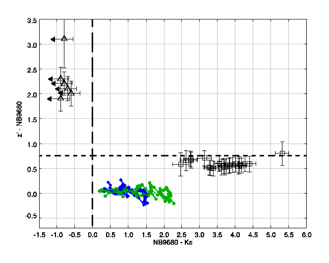
Figure 3: Color-Color Diagram $z^{\prime}$-$NB9680$ vs $NB9680$-Ks showing our criteria $mag_{NB9680}-mag_{z^{\prime}}<-0.75mag$ (short dashed line) and $mag_{NB9680}-mag_{Ks}<0mag$ (long dashed line). The empty triangle symbol correspond to the LAE candidates. The empty squares represent the L-T-Dwarfs from Dahn et al. (2002). The green track represents early-type galaxies and the blue track dusty galaxies generated with Bruzual & Charlot (2003).

We also report in Table 3 the lower limits of the rest-frame equivalent widths ($EW$) derived from the photometric data following Malhotra & Rhoads (2002), defined as:

$$EW_{\mathrm{rest}}(\AA)=\left(\frac{f_{NB9680}\Delta\lambda_{Z}-f_{Z}\Delta\lambda_{NB9680}}{f_{Z}-f_{NB9680}}\right)\times\frac{1}{1+z}$$ (2)

where $f_{NB9680}$ is the observed flux in the narrow-band combined image, $f_{Z}$ is the observed flux in the $z^{\prime}$ broad-band image, $\Delta\lambda_{NB9680}$ and $\Delta\lambda_{Z}$ are the width of the $NB9680$ filter (90Å) and the $z^{\prime}$ band filter (928Å) respectively.
Our first object, LAE#1 in Table 3, present a detection in Ks band (see Figure 4). This could be due to a very red continuum slope. However, looking at the Spitzer/IRAC data in 3.5$\mu$m and 4.8$\mu$m, none of the LAE candidates are detected. Alternatively, it could be due to the presence of another line, such as MgII. Looking at the UKIRT/WFCAM2 data in J band ($J_{50\%}=25.6$, AB, 5$\sigma$) for all our high redshift candidates, LAE#1 is detected in this data with a magnitude of 24.8 (AB) and a SNR(J)$\sim$ 10. From the HST/NICMOS data available in H band ($H_{50\%}=26.7$, AB, 5$\sigma$), LAE#3 is detected with a magnitude of 26.5 and a SNR(H)$\sim$4.
These detections in different broad bands confirm the reliability on these candidates. Although the other candidates have a strong single band detection, the tests realized in Paragraph  3.2.1 confirm that they are emission line objects. The remaining candidates are based on a $\geq 5\sigma$ significant single-band detection in the narrow band filter. For Gaussian statistics, the false positive probability at $\geq 5\sigma$ is $3\times 10^{-7}$, while our survey area contains $\sim 0.5\times 10^{7}$ independent resolution elements (based on $0.65^{\prime\prime}$ seeing). The number of noise spikes entering the sample should thus be $\sim 1.5$, comparable to the expected number of foreground emitters. Non-Gaussian noise could increase this number, but the absence of detections in the negative-image test (see Section 3.2.1) support the conclusion that $5\sigma$ noise spikes are not a major contaminant of our sample.

Three out of six of our LAE photometric candidates are not detected in the $z^{\prime}$ band and we therefore use the detection limit in this band, deriving in turn lower $EW$ limits.

Table 3: Table of the z$\sim 6.96$ LAE candidates.

Name	Ra	Dec	$NB9680$	Error	SNR ($NB9680$)	$z^{\prime}$	Error	$SNR(z^{\prime})$	$EW^{\mathrm{a}}$ (Å)	$J$	Error
LAE#1	10:00:46.846	02:10:16.01	24.1	0.2	7.3	26.0	0.16	6.6	$\sim$41	$24.8^{\mathrm{b}}$	0.15
LAE#2	10:00:39.104	02:03:02.55	24.1	0.18	7.2	$>$26.4	…	…	$>$61	$>$24.8	…
LAE#3	09:59:50.991	02:12:19.13	24.2	0.2	6.4	$>$26.4	…	2	$>$47	$>$24.8	…
LAE#4	10:00:58.529	02:12:56.51	24.2	0.18	6.1	$>$26.4	…	…	$>$47	$>$24.8	…
LAE#5	10:00:42.528	02:11:30.39	24.3	0.19	6.1	$>$26.4	…	0.2	$>$48	$>$24.8	…
LAE#6	10:00:37.940	02:11:59.28	24.4	0.2	5.6	$>$26.4	…	…	$>$41	$>$24.8	…

• In the restframe

• from UKIRT/WFCAM2 data

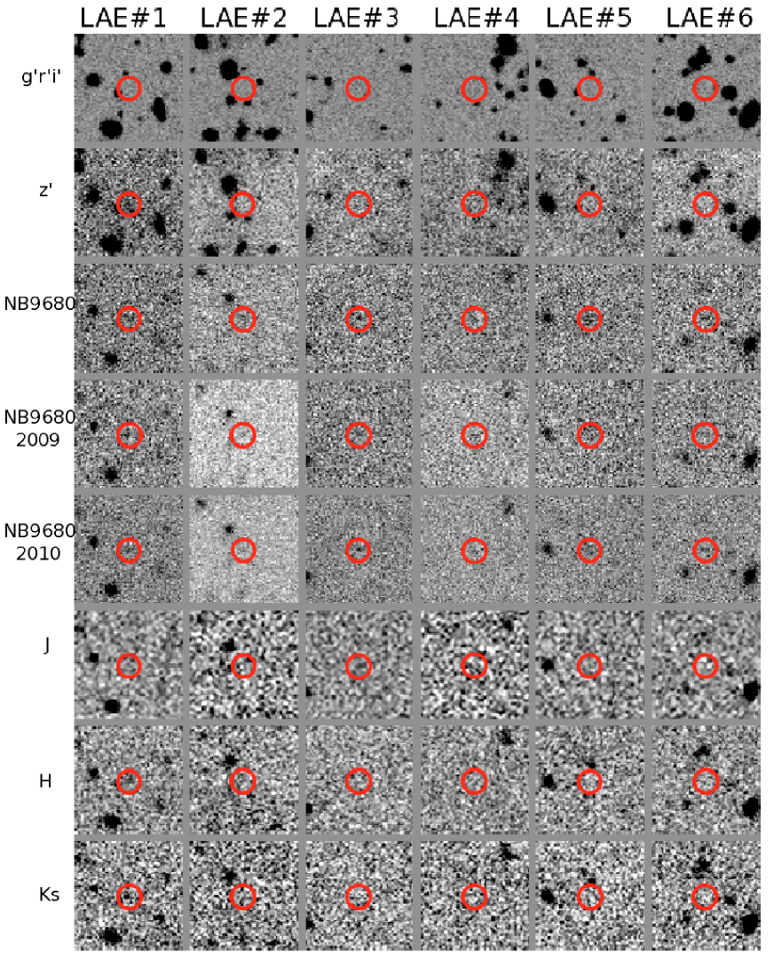
Figure 4: Thumbnail images of all candidates listed in Table 3. Each window is $15^{\prime\prime}\times 15^{\prime\prime}$. Objects names and passbands are located above and to the left of the thumbnails, respectively.

4 Discussion

Variance. Two sources of variance can be involved in a such high redshift study : the Poisson variance and the fluctuations in the large scale distribution of the galaxies, also called the cosmic variance. We used the on-line calculator by Trenti & Stiavelli (2008) to estimate the cosmic variance. This calculator requires numerous parameters such as the area of the survey, the mean redshift, the reshift interval, but also the completeness value and several cosmological parameters. We obtained, for our sample, a value of 54% for the cosmic variance. The Poisson noise is estimated to 58%. The 54% uncertainty from the cosmic variance and the 58% from Poisson statistics are comparable and we therefore consider both in our error estimation.

Luminosity Function. Our $NB9680$ filter being quite narrow (FWHM$\sim$90Å), we assume that the narrow-band flux is entirely coming from the Ly$\alpha$ line. We fit to the Ly$\alpha$ luminosity function of this z$\sim$6.96 LAE sample, a Schechter function, $\Phi(L)$, given by

$$\Phi(L)\mathrm{d}L=\Phi^{*}\left(\frac{L}{L^{*}}\right)^{\alpha}\mathrm{exp}\left(-\frac{L}{L^{*}}\right)\frac{\mathrm{d}L}{L^{*}}$$ (3)

in order to compare with previous high redshift works (Ouchi et al., 2010; Hibon et al., 2010; Tilvi et al., 2010; Ouchi et al., 2008; Ota et al., 2008; Kashikawa et al., 2006; Malhotra & Rhoads, 2004). Considering the small number of candidates in our sample, we choose to fit two out of three of the Schechter function parameters. We set the faint end slope of the luminosity, $\alpha$, to $\alpha=-1.5$, and determine $\Phi^{*}$ and $L^{*}$ by $\chi^{2}$ minimization. We decide to obtain a best-fit Schechter functions for the z$\sim$7 cumulative luminosity function, which has been derived by considering only our photometric candidates.
In Figure 5, we present the Ly$\alpha$ Luminosity Function not corrected for detection incompleteness as a black solid line. We then use the completeness result of Section 2.2.1 to correct the luminosity of our objects, and find a new Schechter fit, presented as a red solid line in Figure 5. This is the z 7 Ly$\alpha$ Luminosity Function corrected for incompleteness.

Table 4: Best fit Schechter LF parameters for $\alpha=-1.5$

Redshift	$\mathrm{log}(L^{*}(\mathrm{erg}\,\mathrm{s}^{-1}))$	$\mathrm{log}(\Phi^{*}(\mathrm{Mpc}^{-3}))$
6.96(1)	$42.56^{+0.1}_{-0.2}$	$-2.01^{+0.15}_{-0.2}$
6.96(2)	$42.8^{+0.12}_{-0.14}$	$-3.44^{+0.20}_{-0.16}$
6.5(3)	$42.64^{+0.1}_{-0.1}$	$-3.07^{+0.13}_{-0.13}$
5.7(4)	$42.8^{+0.16}_{-0.16}$	$-3.11^{+0.29}_{-0.31}$

• (1) derived for our sample; (2)Ota et al. (2008); (3) Ouchi et al. (2010); (4) Ouchi et al. (2008)

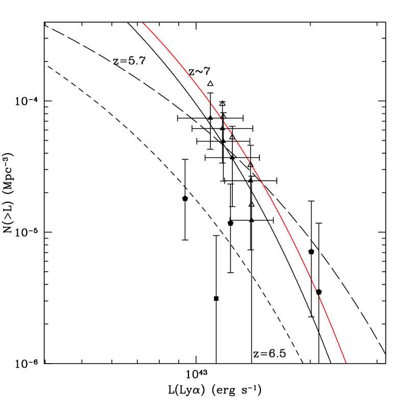
Figure 5: Best-fit Schechter function for the cumulative z$\sim$7 Ly$\alpha$ luminosity function. The red solid line is the best-fit z$\sim$7 LF with completeness correction. Our candidates are represented as triangles (plain: not corrected for completeness, empty : with completeness correction). The error bars represent the Poisson errors and are identical for plain and empty points. The z$\sim$6.96 LAE from Iye et al. (2006) is the square, Ota et al. (2010) candidates are pentagons. Also represented here is the z=6.5 Ly$\alpha$ LF from Ouchi et al. (2010) and the z=5.7 Ly$\alpha$ LF from Ouchi et al. (2008).

Sample Incompleteness. We create a grid pattern of 15000 objects on a mock image, andrun SExtractor for different photometric apertures in double image mode, using the $g^{\prime}$-band image as the measurement image. We remark that by increasing the photometric aperture size, the number of objects matching the optical criterion (Criterion #2 in Table 2) decreases. For an aperture of 5 pixels, we recover 75%$\pm$0.65%, for 10 pixels 63%$\pm$0.6% and for 20 pixels 46%$\pm$0.5%. We choose a photometric aperture of 5 pixels for the objects catalogs we used for the high redshift LAEs selection. We know then that we could miss 25% of the objects due to the photometric aperture size we choose. This corresponds to the possibility that we missed $\sim$1.5 objects in our high redshift sample. Assuming one more object in our sample, our conclusion about the best-fit LF will not change.

Interpretation. The previous studies presenting z$\sim$7 Ly$\alpha$ emitters (Ota et al., 2008, 2010) has lead to the first spectroscopic confirmed z$\sim$7 LAE, called IOK1. Their survey covers an area of 876 square arcmin with the filter NB973 ($\Delta\lambda=200\AA$, $\lambda_{c}=9755\AA$) and reaches a 50% completeness of NB973=25.6 (AB, $5\sigma$) (equivalent to a flux of $1.36e^{-17}\mathrm{erg}\,\mathrm{s}^{-1},\mathrm{cm}^{-2}$) in the SXDS (Subaru/XMM-Newton Deep Survey) and NB973=25.3 (AB, $5\sigma$) (equivalent to a flux of $1.8e^{-17}\mathrm{erg}\,\mathrm{s}^{-1},\mathrm{cm}^{-2}$) in the SDF (Subaru Deep Field). IOK-1 has a flux of $2\times 10^{-17}\mathrm{erg}\,\mathrm{s}^{-1}\,\mathrm{cm}^{-2}$. From the Table 1 of Ota et al. (2008), we are able to obtain a lower limit for the rest-frame equivalent width of IOK1, $EW_{rest}\sim 49\AA$, using Equation  2. This rest-frame equivalent width is in agreement with the rest-frame equivalent limit lower limit we found for our candidate sample and presented in Table  3. Ota et al. (2010) find four new photometric candidates in a survey covering the Subaru/XMM Newton Deep Survey Field with Suprime-Cam and reaching a depth limit of NB973=25.4, corresponding to 72% completeness. These candidates are represented by pentagons in the Figure  5.

From Yoshida et al. (2006), Ota et al. (2008) estimated therefore a possible z$\sim$7 Ly$\alpha$ LF with a pure luminosity evolution of $L^{*}_{z=7}=0.58L^{*}_{z=5.7}$, with $L^{*}_{z=5.7}=1.08.10^{43}\mathrm{erg}\,\mathrm{s}^{-1}$ (Shimasaku et al., 2006). This inferred z$\sim$7 Ly$\alpha$ LF predicts fewer LAEs than seen in our photometric candidate sample. Confirmation of 1-2 of our candidates would approximately match the prediction in Ota et al. (2008) and would modestly exceed their measured number density.

We show in Figure 5 the cumulative z$\sim$7 LAEs LF obtained after correcting our points for the aperture and the detection completeness. This completeness correction has been applied by number weighting according to the NB9860 magnitude. The best-fit parameters do not vary significantly before and after correcting from the completeness, as seen in Figure 5 between the black solid line and the red solid line (without and with the completeness correction, respectively).
By considering only our photometric candidate sample, we do not observe any strong $L^{*}$ or $\Phi^{*}$ evolution between z=5.7 and z$\sim$7, and therefore contradict a possible $L^{*}$ evolution between z=6.5 and z$\sim$7. If none of our candidates is a real z$\sim$7 LAE, we can then put an upper limit on the z$\sim$7 Ly$\alpha$ LF, which will help constrain the neutral fraction of the IGM.

5 Conclusions

We observed 465 $\mathrm{arcmin}^{2}$ from the COSMOS field using the narrow-band imaging technique on Magellan/IMACS with the $NB9680$ filter, in order to target the Ly$\alpha$ line at z$\sim$6.96. We obtained a comoving volume of $\sim 72000Mpc^{3}$. After applying our selection criteria and verifying that our selection was not contaminated by low-redshift emitters and transient objects, we obtain a sample of six z$\sim$6.96 LAEs. From this photometric sample, we are able to infer a possible z$\sim$6.96 Ly$\alpha$ Luminosity Function. We find no evolution in luminosity function from z=6.5 to z$\sim$6.96, if a majority of our sources are confirmed.
It is now crucial to obtain spectroscopic follow-up observations to reveal the real nature of these objects and establish a firm conclusion on the z$\sim$6.96 Ly$\alpha$ Luminosity Function.

References

- Bertin & Arnouts (1996) Bertin, E. & Arnouts, S. 1996, A&AS, 117, 393
- Bruzual & Charlot (2003) Bruzual, G. & Charlot, S. 2003, MNRAS, 344, 1000
- Cassata et al. (2010) Cassata, P., Le Fevre, O., Garilli, B., Maccagni, D., Le Brun, V., Scodeggio, M., Tresse, L., Ilbert, O., Zamorani, G., Cucciati, O., Contini, T., Bielby, R., Mellier, Y., McCracken, H. J., Pollo, A., Zanichelli, A., Bardelli, S., Cappi, A., Pozzetti, L., Vergani, D., & Zucca, E. 2010, ArXiv e-prints
- Cimatti et al. (2002) Cimatti, A., Daddi, E., Mignoli, M., Pozzetti, L., Renzini, A., Zamorani, G., Broadhurst, T., Fontana, A., Saracco, P., Poli, F., Cristiani, S., D’Odorico, S., Giallongo, E., Gilmozzi, R., & Menci, N. 2002, A&A, 381, L68
- Cuby et al. (2007) Cuby, J., Hibon, P., Lidman, C., Le Fèvre, O., Gilmozzi, R., Moorwood, A., & van der Werf, P. 2007, A&A, 461, 911
- Dahn et al. (2002) Dahn, C. C., Harris, H. C., Vrba, F. J., Guetter, H. H., Canzian, B., Henden, A. A., Levine, S. E., Luginbuhl, C. B., Monet, A. K. B., Monet, D. G., Pier, J. R., Stone, R. C., Walker, R. L., Burgasser, A. J., Gizis, J. E., Kirkpatrick, J. D., Liebert, J., & Reid, I. N. 2002, AJ, 124, 1170
- Furlanetto et al. (2006) Furlanetto, S. R., Zaldarriaga, M., & Hernquist, L. 2006, MNRAS, 365, 1012
- Geach et al. (2010) Geach, J. E., Cimatti, A., Percival, W., Wang, Y., Guzzo, L., Zamorani, G., Rosati, P., Pozzetti, L., Orsi, A., Baugh, C. M., Lacey, C. G., Garilli, B., Franzetti, P., Walsh, J. R., & Kümmel, M. 2010, MNRAS, 402, 1330
- Hibon et al. (2010) Hibon, P., Cuby, J., Willis, J., Clément, B., Lidman, C., Arnouts, S., Kneib, J., Willott, C. J., Marmo, C., & McCracken, H. 2010, A&A, 515, A97+
- Hu et al. (2002) Hu, E. M., Cowie, L. L., McMahon, R. G., Capak, P., Iwamuro, F., Kneib, J., Maihara, T., & Motohara, K. 2002, ApJ, 568, L75
- Iye et al. (2006) Iye, M., Ota, K., Kashikawa, N., Furusawa, H., Hashimoto, T., Hattori, T., Matsuda, Y., Morokuma, T., Ouchi, M., & Shimasaku, K. 2006, Nature, 443, 186
- Kakazu et al. (2007) Kakazu, Y., Cowie, L. L., & Hu, E. M. 2007, ApJ, 668, 853
- Kashikawa et al. (2006) Kashikawa, N., Shimasaku, K., Malkan, M. A., Doi, M., Matsuda, Y., Ouchi, M., Taniguchi, Y., Ly, C., Nagao, T., Iye, M., Motohara, K., Murayama, T., Murozono, K., Nariai, K., Ohta, K., Okamura, S., Sasaki, T., Shioya, Y., & Umemura, M. 2006, ApJ, 648, 7
- Malhotra & Rhoads (2002) Malhotra, S. & Rhoads, J. E. 2002, ApJ, 565, L71
- Malhotra & Rhoads (2004) —. 2004, ApJ, 617, L5
- Malhotra & Rhoads (2006) —. 2006, ApJ, 647, L95
- Malhotra et al. (2011) Malhotra, S., Rhoads, J. E., Finkelstein, S., Hathi, N., Nilsson, K., McLinden, E., & Pirzkal, N. 2011, Submitted to ApJ
- McCracken et al. (2010) McCracken, H. J., Capak, P., Salvato, M., Aussel, H., Thompson, D., Daddi, E., Sanders, D. B., Kneib, J., Willott, C. J., Mancini, C., Renzini, A., Cook, R., Le Fèvre, O., Ilbert, O., Kartaltepe, J., Koekemoer, A. M., Mellier, Y., Murayama, T., Scoville, N. Z., Shioya, Y., & Tanaguchi, Y. 2010, ApJ, 708, 202
- Ota et al. (2008) Ota, K., Iye, M., Kashikawa, N., Shimasaku, K., Kobayashi, M., Totani, T., Nagashima, M., Morokuma, T., Furusawa, H., Hattori, T., Matsuda, Y., Hashimoto, T., & Ouchi, M. 2008, ApJ, 677, 12
- Ota et al. (2010) Ota, K., Iye, M., Kashikawa, N., Shimasaku, K., Ouchi, M., Totani, T., Kobayashi, M. A. R., Nagashima, M., Harayama, A., Kodaka, N., Morokuma, T., Furusawa, H., Tajitsu, A., & Hattori, T. 2010, ArXiv e-prints
- Ouchi et al. (2008) Ouchi, M., Shimasaku, K., Akiyama, M., Simpson, C., Saito, T., Ueda, Y., Furusawa, H., Sekiguchi, K., Yamada, T., Kodama, T., Kashikawa, N., Okamura, S., Iye, M., Takata, T., Yoshida, M., & Yoshida, M. 2008, ApJS, 176, 301
- Ouchi et al. (2010) Ouchi, M., Shimasaku, K., Furusawa, H., SAITO, T., Yoshida, M., Akiyama, M., Ono, Y., Yamada, T., Ota, K., Kashikawa, N., Iye, M., Kodama, T., Okamura, S., Simpson, C., & Yoshida, M. 2010, ArXiv e-prints
- Regnault et al. (2009) Regnault, N., Conley, A., Guy, J., Sullivan, M., Cuillandre, J., Astier, P., Balland, C., Basa, S., Carlberg, R. G., Fouchez, D., Hardin, D., Hook, I. M., Howell, D. A., Pain, R., Perrett, K., & Pritchet, C. J. 2009, A&A, 506, 999
- Rhoads & Malhotra (2001) Rhoads, J. E. & Malhotra, S. 2001, ApJ, 563, L5
- Rigopoulou et al. (2005) Rigopoulou, D., Vacca, W. D., Berta, S., Franceschini, A., & Aussel, H. 2005, A&A, 440, 61
- Ryan et al. (2005) Ryan, Jr., R. E., Hathi, N. P., Cohen, S. H., & Windhorst, R. A. 2005, ApJ, 631, L159
- Shimasaku et al. (2006) Shimasaku, K., Kashikawa, N., Doi, M., Ly, C., Malkan, M. A., Matsuda, Y., Ouchi, M., Hayashino, T., Iye, M., Motohara, K., Murayama, T., Nagao, T., Ohta, K., Okamura, S., Sasaki, T., Shioya, Y., & Taniguchi, Y. 2006, PASJ, 58, 313
- Spergel et al. (2007) Spergel, D. N., Bean, R., Doré, O., Nolta, M. R., Bennett, C. L., Dunkley, J., Hinshaw, G., Jarosik, N., Komatsu, E., Page, L., Peiris, H. V., Verde, L., Halpern, M., Hill, R. S., Kogut, A., Limon, M., Meyer, S. S., Odegard, N., Tucker, G. S., Weiland, J. L., Wollack, E., & Wright, E. L. 2007, ApJS, 170, 377
- Stern et al. (2005) Stern, D., Yost, S. A., Eckart, M. E., Harrison, F. A., Helfand, D. J., Djorgovski, S. G., Malhotra, S., & Rhoads, J. E. 2005, ApJ, 619, 12
- Straughn et al. (2009) Straughn, A. N., Pirzkal, N., Meurer, G. R., Cohen, S. H., Windhorst, R. A., Malhotra, S., Rhoads, J., Gardner, J. P., Hathi, N. P., Jansen, R. A., Grogin, N., Panagia, N., di Serego Alighieri, S., Gronwall, C., Walsh, J., Pasquali, A., & Xu, C. 2009, AJ, 138, 1022
- Tilvi et al. (2010) Tilvi, V., Rhoads, J. E., Hibon, P., Malhotra, S., Wang, J., Veilleux, S., Swaters, R., Probst, R., Krug, H., Finkelstein, S. L., & Dickinson, M. 2010, ArXiv e-prints
- Tinney et al. (2003) Tinney, C. G., Burgasser, A. J., & Kirkpatrick, J. D. 2003, AJ, 126, 975
- Trenti & Stiavelli (2008) Trenti, M. & Stiavelli, M. 2008, ApJ, 676, 767
- Tresse et al. (2002) Tresse, L., Maddox, S. J., Le Fèvre, O., & Cuby, J.-G. 2002, MNRAS, 337, 369
- Willis et al. (2008) Willis, J. P., Courbin, F., Kneib, J., & Minniti, D. 2008, MNRAS, 384, 1039
- Yoshida et al. (2006) Yoshida, M., Shimasaku, K., Kashikawa, N., Ouchi, M., Okamura, S., Ajiki, M., Akiyama, M., Ando, H., Aoki, K., Doi, M., Furusawa, H., Hayashino, T., Iwamuro, F., Iye, M., Karoji, H., Kobayashi, N., Kodaira, K., Kodama, T., Komiyama, Y., Malkan, M. A., Matsuda, Y., Miyazaki, S., Mizumoto, Y., Morokuma, T., Motohara, K., Murayama, T., Nagao, T., Nariai, K., Ohta, K., Sasaki, T., Sato, Y., Sekiguchi, K., Shioya, Y., Tamura, H., Taniguchi, Y., Umemura, M., Yamada, T., & Yasuda, N. 2006, ApJ, 653, 988