Three Dimensional Flow of Colloidal Glasses

Abstract

Recent experiments performed on a variety of soft glassy materials have demonstrated that any imposed shear flow serves to simultaneously fluidize these systems in all spatial directions [Ovarlez et al. (2010)]. When probed with a second shear flow, the viscous response of the experimental system is determined by the rate of the primary, fluidizing flow. Motivated by these findings, we employ a recently developed schematic mode-coupling theory [Brader et al. (2009)] to investigate the three dimensional flow of a colloidal glass, subject to a combination of simple shear and uniaxial compression. Despite differences in the specific choice of superposed flow, the flow curves obtained show good qualitative agreement with the experimental findings and recover the observed power law describing the decay of the scaled viscosity as a function of the dominant rate. We then proceed to perform a more formal analysis of our constitutive equation for different kind of ‘mixed’ flows consisting of a dominant primary flow subject to a weaker perturbing flow. Our study provides further evidence that the theory of Brader et al. (2009) reliably describes the dynamic arrest and mechanical fluidization of dense particulate suspensions.

I Introduction

Colloidal dispersions display a broad range of nontrivial rheological response to externally applied flow. Even the simplest systems of purely repulsive spherical colloids exhibit a rate dependent viscosity in steady state flows, yielding and complex time-dependent phenomena, such as thixotropy and ageing [Brader (2010), Mewis and Wagner (2009)]. Understanding the emergence of these collective dynamical phenomena from the underlying interparticle interactions poses a challenge to nonequilibrium statistical mechanics and the fundamental mechanisms involved are only beginning to be understood. Theoretical advances have largely been made hand-in-hand with improved simulation techniques [Banchio and Brady (2003)] and modern experimental developments, combining confocal microscopy or magnetic resonance imaging with classical rheological measurements [Besseling et al. (2010), Frank et al. (2003)].

Despite considerable progress, a comprehensive constitutive theory, capable of capturing the full range of response, remains to be found. Existing approaches are tailored to capture the physics of interest within particular ranges of the system parameters (e.g. density, temperature) but fail to provide the desired global framework. Moreover, the vast majority of studies have concentrated on the specific, albeit important, case of simple shear flow. Such scalar constitutive theories, relating the shear stress to the shear strain and/or strain-rate, provide important information regarding the competition of timescales underlying the rheological response, but do not acknowledge the true three dimensional character of experimental flows. Tensorial constitutive equations have long been a staple of continuum rheology (such as the Giesekus or Oldroyd models [Bird et al. (1987), Larson (1988)]) and enable e.g. normal forces and secondary flows to be addressed in realistic curvilinear experimental geometries.

The first steps towards a unified, three dimensional description of colloid rheology have been provided by recent extensions of the quiescent mode-coupling theory (MCT) to treat dense dispersions under flow [Brader et al. (2008)]. These developments are built upon earlier studies focused on simple shear [Brader et al. (2007), Fuchs (2009), Fuchs and Cates (2002), Fuchs and Cates (2009)] and capture the competition between slow structural relaxation and external driving, thus enabling one of the most challenging aspects of colloid rheology to be addressed: the flow response of dynamically arrested glass and gel states. Given the equilibrium static structure factor as input (available from either simulation or liquid state theory [Brader (2006)]), the deviatoric stress tensor $\boldsymbol{\sigma}(t)$ may be determined for any given velocity gradient tensor $\boldsymbol{\kappa}(t)$. However, implementation of the theory has been hindered by the numerical resources required to accurately integrate fully anisotropic dynamics over timescales of physical interest (although progress has been made for two dimensional systems [Henrich et al. (2009), Krüger et al. (2011)]). In [Brader et al. (2009)] a simplified ‘schematic’ constitutive model was proposed, which aims to capture the essential physics of the wavector dependent theory, while remaining numerically tractable. Applications so far have been to steady-state flows, step strain and dynamic yielding [Brader et al. (2009)], as well as oscillatory shear [Brader et al. (2010)].

Both the full [Brader et al. (2008)] and schematic [Brader et al. (2009)] mode-coupling theories predict an idealized glass transition at sufficiently high coupling strength, characterized by an infinitely slow structural relaxation time $\tau_{\alpha}$. Ageing dynamics are neglected. An important prediction of the approach is that application of any steady strain-rate leads to fluidization of the arrested microstructure, with a structural relaxation time determined by the characteristic rate of flow $\tau_{\alpha}\sim\dot{\gamma}^{-1}$.

In recent experiments on various soft glassy materials, Ovarlez et al. have indicated that when a dominant, fluidizing shear flow is imposed, then the sample responds as a liquid to an additional perturbing shear flow, regardless of the spatial direction in which this perturbation is applied. These findings imply that once the yield stress has been overcome by the dominant shear flow, arrested states of soft matter become simultaneously fluidized in all spatial directions. In particular, the low shear viscosity in a direction orthogonal to the primary flow is determined by the primary flow rate. The rheometer employed in [Ovarlez (2010)] consisted of two parallel discs which enabled the simultaneous application of rotational and squeeze shear flow, with independent control over the two different shear rates. Although this set-up indeed provides a useful way to study superposed shear flows of differing rate, it does not provide a mean to test the three-dimensional yield surface, as claimed in [Ovarlez (2010)]. A true exploration of the yield surface poses a considerable challenge to experiment and requires a parameterization of the velocity gradient tensor which can incorporate the entire family of homogeneous flows, including both extension and shear as special cases. The superposition of two shear flows is yet another shear flow and does not enable the entire space of homogeneous velocity gradients to be explored.

In the present work we will employ the constitutive theory of Brader et al. (2009) to investigate the response of a generic colloidal glass to a ‘mixed’ flow described mathematically by the linear superposition of two independently controllable velocity gradient tensors. Numerical results will be presented for the special case in which simple shear is combined with uniaxial compression. Despite the fact that we employ a combination of compression and shear, as opposed to the superposition of two shear flows, our theoretical results are broadly consistent with the experimental findings of Ovarlez et al. (2010) regarding the response of shear fluidized glasses. In particular, our calculations reveal clearly the relevant timescales dictating the three dimensional response of the system. Following this specific application, we proceed to extend our description to treat more general mixed flows.

The paper will be organized as follows: In Sec. II we will introduce the deformation measures required to describe flow in three dimensions and summarize the schematic model of Brader et al. (2009). In Sec. III we will consider the application of our constitutive model to a specific mixed flow, namely a combination of uniaxial compression and simple shear. In Sec. IV we will present numerical results for the flow curves and low shear viscosity for the aforementioned flow combination. In Sec. V we will perform a perturbation analysis of our constitutive equation which enables us to address the general problem of superposing a mechanical perturbation onto a dominant flow. Finally, in Sec. VI we will discuss the significance of our results and give concluding remarks.

II The schematic model

II.1 Continuum tensors

Spatially homogeneous deformations are encoded in the spatially translationally invariant deformation tensor $\boldsymbol{E}(t,t^{\prime})$. Any given vector $\boldsymbol{r}(t^{\prime})$ at time $t^{\prime}$ may be transformed into a new vector $\boldsymbol{r}(t)$ at later time $t$ using the linear relation

$$\boldsymbol{r}(t)=\boldsymbol{E}(t,t^{\prime})\cdot\boldsymbol{r}(t^{\prime})\,,$$ (1)

where $E_{\alpha\beta}=\partial r_{\alpha}(t)/\partial r_{\beta}(t^{\prime})$ [Brader (2010)]. Calculating the time derivative of the deformation tensor $\boldsymbol{E}$ and using the chain rule for derivatives yields an equation of motion for the deformation tensor

$$\frac{\partial\boldsymbol{E}(t,t^{\prime})}{\partial t}=\boldsymbol{\kappa}(t)\cdot\boldsymbol{E}(t,t^{\prime})\,,$$ (2)

where $\boldsymbol{\kappa}=\nabla\boldsymbol{v}$ is the velocity gradient tensor with components $(\nabla\boldsymbol{v})_{\alpha\beta}=\partial\dot{r}_{\alpha}/\partial r_{\beta}$. In the present work we will assume incompressibility, which may be expressed by the condition ${\rm Tr}\,\boldsymbol{\kappa}=0$ or, equivalently, ${\rm Tr}\,\boldsymbol{E}=1$ (volume is conserved). If the deformation rate is constant in time, then the velocity gradient matrix $\boldsymbol{\kappa}$ loses its time dependence ($\boldsymbol{\kappa}(t)\rightarrow\boldsymbol{\kappa}$) and the deformation tensor $\boldsymbol{E}$ becomes a function of the time difference alone ($\boldsymbol{E}(t,t^{\prime})\rightarrow\boldsymbol{E}(t-t^{\prime})$). The formal solution of Eq.(2) for such steady flows is thus given by

$$\boldsymbol{E}(t)=e^{\boldsymbol{\kappa}t}\,.$$ (3)

The deformation tensor contains information about both the stretching and rotation of material lines (vectors embedded in the material). A more useful measure of strain is the Finger tensor $\boldsymbol{B}(t,t^{\prime})$, which is defined for steady flows by

$$\boldsymbol{B}(t)=\boldsymbol{E}(t)\cdot\boldsymbol{E}^{T}(t)\,.$$ (4)

The Finger tensor is invariant with respect to physically irrelevant solid body rotations of the material sample and occurs naturally in many constitutive models (e.g. the Doi-Edwards model of polymer melts [Doi and Edwards (1989)]).

II.2 Schematic mode-coupling equations

The schematic model developed in [Brader et al. (2009)] expresses the deviatoric stress tensor in integral form

$$\boldsymbol{\sigma}(t)=\int_{-\infty}^{t}\!\!dt^{\prime}\Big{[}-\frac{\partial}{\partial t^{\prime}}\boldsymbol{B}(t,t^{\prime})\Big{]}G(t,t^{\prime})\,.$$ (5)

An equation of the form (5) has been derived from first principles [Brader et al. (2008)], starting from the $N$-particle Smoluchowski equation and applying mode-coupling approximations to a formally exact generalized Green-Kubo relation for the stress tensor. In [Brader et al. (2009)] the theory was simplified to (5) by assuming spatial isotropy of the modulus $G(t,t^{\prime})$. The physical content of Eq.(5) is that, in order to calculate the stress at the present time, increments of an appropriate, material objective strain measure (the Finger tensor) are integrated over the flow history, each weighted with a ‘fading memory’. Approximating $G(t,t^{\prime})$ by an exponential recovers the well-known Lodge equation [Larson (1988)], which is just the integral form of the upper-convected Maxwell model. However, Eq.(5) differs from the simple Lodge equation in that, (i) the modulus $G$ is generally not time translationally invariant, due time-dependent variation of the flow in the time interval between $t$ and $t^{\prime}$, (ii) the memory does not decay exponentially to zero, but displays the two-step relaxation characteristic of dense colloidal dispersions.

Within the wavevector dependent approach of [Brader et al. (2008)] the autocorrelation function of stress fluctuations is assumed to relax in the same way as the density fluctuations. This leads to an approximation for the nonlinear modulus $G$, given by a weighted ${\bf k}$-integral over a bilinear function of density correlators at two different (but coupled) wavevectors. The schematic model replaces this with the simpler form

$$G(t,t^{\prime})=\nu_{\sigma}\Phi^{2}(t,t^{\prime})\,,$$ (6)

where $\Phi(t,t^{\prime})$ is a single mode transient density correlator (normalized to $\Phi(t,t)=1$) and $\nu_{\sigma}$ is a parameter measuring the strength of stress fluctuations.

The dynamics of the single mode density correlator are determined by a nonlinear integro-differential equation

$$\dot{\Phi}(t,t_{0})+\Gamma\Bigg{\{}\Phi(t,t_{0})+\int_{t_{0}}^{t}dt^{\prime}m(t,t^{\prime},t_{0})\dot{\Phi}(t^{\prime},t_{0})\Bigg{\}}=0\,,$$ (7)

where $\Gamma$ is an initial decay rate, the inverse of which sets our basic unit of time. The function $m(t,t^{\prime},t_{0})$ is a three-time memory-kernel which depends upon the strain accumulated between its time arguments and describes how this competes with the slow structural relaxation arising from the colloidal interactions. The memory kernel is given by

$$m(t,t^{\prime},t_{0})=h_{1}(t,t_{0})h_{2}(t,t^{\prime})\Bigg{[}\nu_{1}\Phi(t,t^{\prime})+\nu_{2}\Phi^{2}(t,t^{\prime})\Bigg{]}\,.$$ (8)

The dependence of the memory upon $\Phi(t,t^{\prime})$ is taken from the $F_{12}$ model developed by Götze [Götze (2008)]. The coupling constants are given by $\nu_{1}=2(\sqrt{2}-1)+\varepsilon/(\sqrt{2}-1)$ and $\nu_{2}=2$, where $\varepsilon$ is a parameter expressing the distance to the glass transition. The system is fluid for $\varepsilon<0$ and in a glassy state for $\varepsilon>0$.

The $h_{i}$ entering (8) are decaying functions of the accumulated strain. For simplicity we assume $h_{1}=h_{2}=h$. To allow consideration of any kind of flow (not only shear), the function $h$ is taken to depend upon the two invariants $I_{1}$ and $I_{2}$ of the Finger tensor

$$h(t,t_{0})=\frac{\gamma_{\rm cr}^{2}}{\gamma_{\rm cr}^{2}+\Big{[}\nu I_{1}(t,t_{0})+(1-\nu)I_{2}(t,t_{0})-3\Big{]}}\,,$$ (9)

where a mixing parameter $(0\leq\nu\leq 1)$ and a cross-over strain parameter $(\gamma_{\rm cr})$ have been introduced [Brader et al. (2009)]. The scalars $I_{1}=Tr(\boldsymbol{B})$ and $I_{2}=Tr(\boldsymbol{B}^{-1})$ are the trace of the Finger tensor and its inverse, respectively. In principle, the time evolution of the density correlator $\Phi(t,t_{0})$ and thus, via Eqs.(5) and (6), the stress tensor, can be calculated by solving Eq.(7) numerically for any given velocity gradient tensor $\boldsymbol{\kappa}$.

The model outlined above contains a set of five independent parameters $(v_{\sigma},\Gamma,\varepsilon,\nu,\gamma_{\rm cr})$. The least important of these is $\nu$, which determines the relative influence of the invariant $I_{1}$ with respect to $I_{2}$ in determining the strain induced decay of the memory function. However, numerical results prove to be extremely insensitive to the value of $\nu$, at least for all flows to which the schematic model has so far been applied.

Trivial scaling of stress and time scales is provided by the parameters $v_{\sigma}$ and $\Gamma$. A statistical mechanical calculation of the dynamics of $N$ colloids (in the absence of hydrodynamic interactions) identifies the modulus $G$ as the autocorrelation function of stress fluctuations. $v_{\sigma}$ therefore determines the initial value of the modulus and, via (5), sets the overall stress scale. The reciprocal of the initial decay rate $\Gamma^{-1}$ simply acts as the fundamental timescale. For the purpose of our theoretical investigations both $v_{\sigma}$ and $\Gamma$ can, without loss of generality, be set equal to unity. The theoretical results thus generated can then be fit to experimental data by scaling stress and time (or frequency) with alternative values for these two parameters [Brader et al. (2010)]

The two most important parameters in the model are $\gamma_{\rm cr}$ and $\varepsilon$. The cross-over strain $\gamma_{\rm cr}$ sets the strain value at which elastic response gives way to viscous flow. For example, in experiments considering the shear stress response of dense colloidal systems to the onset of steady shear flow, $\gamma_{\rm cr}$ can be identified from the peak of the overshoot on the stress-strain curve. The parameter $\varepsilon$ characterizes the thermodynamic state point of the system relative to the glass transition and serves as proxy for the true thermodynamic parameters of the physical system (volume fraction, temperature etc.). For example, in a simple system of hard-sphere colloids of volume fraction $\phi$ one can identify $\varepsilon\sim(\phi-\phi_{\rm g})/\phi_{\rm g}$, where $\phi_{\rm g}$ is the volume fraction at the glass transition. For more complicated systems $\varepsilon$ can be regarded as a general coupling parameter which, in the absence of flow, yields fluid-like behaviour for $\varepsilon<0$ and amorphous solid-like response for $\varepsilon>0$.

III Mixed shear and compressional flows

With the constitutive relation (5), we are in a position to determine the rheological behaviour of a colloidal glass undergoing any type of homogeneous deformation. In [Ovarlez et al. (2010)], Ovarlez et al. considered various soft glassy materials loaded between two parallel discs. Each sample was simultaneously sheared by rotating the upper disc about its axis at a given angular velocity and squeezed by lowering the height of the upper disc at a given rate. By independently varying the rotation and compression rates the stress could be determined as a function of one of the rates, for a fixed value of the other. In these experiments, the rotation of the upper plate induces a shear flow in the $\hat{{\boldsymbol{\phi}}}$ direction (in cylindrical coordinates), the rate of which increases linearly with radial distance from the axis of rotation. As a consequence of the stick boundary conditions the compression of the sample leads to an inhomogeneous shear flow in the $\hat{{\bf r}}$ direction (somewhat akin to a Poiseuille flow) with a maximum shear rate at the boundaries and zero shear rate in the plane equidistant between the two plates.

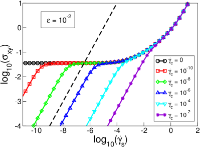
Figure 1: The flow curves of a glassy state ($\varepsilon>0$) for various values of the compressional rate $\dot{\gamma}_{c}$. The dashed line is a Newtonian viscous law. For $\dot{\gamma}_{c}=0$ the $\dot{\gamma}_{s}\rightarrow 0$ limit of the flow curve identifies the dynamic yield stress [Brader et al. (2009)].

The experiments of Ovarlez et al. (2010) were performed in a curvilinear geometry using a flow protocol which induces an inhomogeneous velocity gradient tensor. In principle, spatial variations of the velocity gradient could be treated within the present theoretical framework by assuming that the constitutive relations remain valid locally and enforcing the local stress balance appropriate to the geometry of the rheometer under consideration. In addition to the increased numerical resources required for such an investigation, the local application of our constitutive equation would represent a further approximation, over and above those already underlying the schematic model. The main conceptual point emerging from the experimental studies of Ovarlez et al. (2010) is that if a primary flow restores ergodicity and fluidizes the glass, then the response to the secondary flow is also fluid like. Spatial inhomogeneity of one or both flows is merely a complicating factor. We thus choose to focus on a more idealized homogeneous flow which is convenient for numerical implementation, but nevertheless captures the salient features of the experiment in a minimal way.

The homogeneous flow we choose to implement is a superposition of simple shear and uniaxial compressional flow. We anticipate that the key physical mechanism at work in fluidized systems under superposed flow is the competition between the two imposed relaxation timescales. As the superposition of two shear flows is itself another shear flow, the experiments of Ovarlez et al. (2010) leave open the possibility that the observed phenomena could be a special feature of shear. For this reason we chose to implement the mathematically more general case of superposed extension and shear, for which the geometrical coupling of the flows is more involved.

Working in a cartesian coordinate system our flow is specified by

$$\boldsymbol{\kappa}=\boldsymbol{\kappa}_{s}+\boldsymbol{\kappa}_{c}.$$ (10)

The shear and compressional flows are represented by the following matrices

$$\boldsymbol{\kappa}_{s}=\left(\begin{array}[]{ccc}0&\dot{\gamma}_{s}&0\\ 0&0&0\\ 0&0&0\\ \end{array}\right)\quad\quad\boldsymbol{\kappa}_{c}=\left(\begin{array}[]{ccc}\dot{\gamma}_{c}/2&0&0\\ 0&-\dot{\gamma}_{c}&0\\ 0&0&\dot{\gamma}_{c}/2\\ \end{array}\right)$$ (11)

where $\dot{\gamma}_{s}$ and $\dot{\gamma}_{c}$ are the shear and compression rates, respectively. Our choice of flow thus differs from those of Ovarlez in two respects, (i) both $\dot{\gamma}_{s}$ and $\dot{\gamma}_{c}$ are translationally invariant and, (ii) we superpose shear with genuine elongation, as opposed to superposing two shear flows. We consider the flow (10) as a thought experiment intended to highlight the fundamental physical mechanism of fluidization in a simple and transparent fashion. A direct experimental realization of (10) is not feasible, as this would require a rheometer with stick boundary conditions for generating the shear flow, but slip boundaries for the compressional flow. As we will see below, our assumptions do not seem to lead to qualitative differences between our theoretical findings and the experimental results and simplify considerably the theoretical calculations.

Eq.(3) enables calculation of the deformation tensor $\boldsymbol{E}(t)$ for our mixed flow. The non-zero elements are given by

$$E_{xx}=E_{zz}=e^{\dot{\gamma}_{c}t/2}\quad,$$

$$E_{yy}=e^{-\dot{\gamma}_{c}t}\quad,\vspace*{-0.5cm}$$

$$E_{xy}=\frac{2\dot{\gamma}_{s}}{3\dot{\gamma}_{c}}e^{-\dot{\gamma}_{c}t}\left(e^{\frac{3\dot{\gamma}_{c}t}{2}}-1\right)\,.$$ (12)

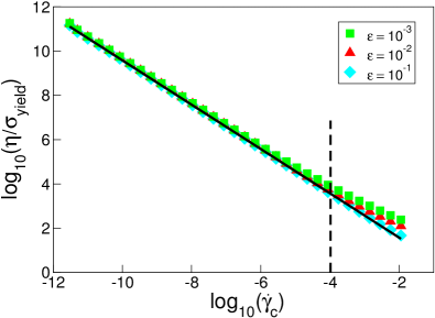
Figure 2: The low shear viscosity $\eta$ scaled by the yield stress $\sigma_{\text{yield}}$ as a function of compression rate $\dot{\gamma}_{c}$ (glassy states with $\varepsilon=10^{-1},10^{-2}$ and $10^{-3}$). The continuous line is a power-law fit to the numerical data points for $\varepsilon=10^{-1}$ over the range $\dot{\gamma}_{c}=10^{-12}-10^{-4}$ and yields an exponent of -1. The $\varepsilon$-dependent deviations apparent for $\dot{\gamma}_{c}>10^{-4}$ indicate that short-time relaxation processes are becoming relevant.

Employing Eq.(4) yields the Finger tensor

$$\boldsymbol{B}(t)=\left(\begin{array}[]{ccc}E_{xx}^{2}+E_{xy}^{2}&E_{xy}E_{yy}&0\\[7.11317pt] E_{xy}E_{yy}&E_{yy}^{2}&0\\[7.11317pt] 0&0&E_{zz}^{2}\end{array}\right)\quad,$$ (13)

with inverse given by

$$\boldsymbol{B}^{-1}(t)=\left(\begin{array}[]{ccc}\frac{1}{E_{xx}^{2}}&\frac{-E_{xy}}{E_{xx}^{2}E_{yy}}&0\\[8.5359pt] \frac{-E_{xy}}{E_{xx}^{2}E_{yy}}&\frac{E_{xx}^{2}E_{zz}^{2}+E_{xy}^{2}E_{zz}^{2}}{E_{xx}^{2}E_{yy}^{2}E_{zz}^{2}}&0\\[8.5359pt] 0&0&\frac{1}{E_{zz}^{2}}\end{array}\right)\quad.$$ (14)

The invariants required for the memory function prefactors (9) are thus

$$I_{1}(t)=2e^{\dot{\gamma}_{c}t}+e^{-2\dot{\gamma}_{c}t}+E_{xy}^{2}\quad,$$ (15)

$$I_{2}(t)=2e^{-\dot{\gamma}_{c}t}+e^{2\dot{\gamma}_{c}t}+E_{xy}^{2}e^{\dot{\gamma}_{c}t}\quad.$$ (16)

Finally, we need to calculate the time derivative of the Finger tensor $\boldsymbol{B}(t)$. In Sec. IV we will present results for the shear stress $\sigma_{xy}$ as a function of $\dot{\gamma}_{s}$, treating $\dot{\gamma}_{c}$ as a parameter. Inspection of (5) shows that we require only the $xy$ component of the Finger tensor time derivative

$$\frac{\partial B_{xy}(t)}{\partial t}=\frac{\dot{\gamma}_{s}}{3}e^{-2\dot{\gamma}_{c}t}\left(4-e^{\frac{3\dot{\gamma}_{c}t}{2}}\right)\quad.$$ (17)

Substituting (17) into (5) and assuming time translational invariance (as appropriate for the steady flows under consideration) we obtain our final expression

$$\sigma_{xy}=\!\int_{0}^{\infty}\!\!\!dt\Bigg{[}\frac{\dot{\gamma}_{s}}{3}e^{-2\dot{\gamma}_{c}t}\left(4-e^{\frac{3\dot{\gamma}_{c}t}{2}}\right)\Bigg{]}\nu_{\sigma}\Phi^{2}(t).$$ (18)

The $xy$ component of the shear stress tensor is now completely characterized. When numerically evaluating the integral in (18) we find that truncation at $\tau\sim(\dot{\gamma}_{s}+\dot{\gamma}_{c})^{-1}$ provides accurate results. We note that, in an analogous way, all other components of the shear stress $\boldsymbol{\sigma}(t)$ can be calculated, which is useful if one is interested for example in the first and second normal stress differences, $N_{1}\equiv\sigma_{xx}-\sigma_{yy}$ and $N_{2}\equiv\sigma_{yy}-\sigma_{zz}$, respectively.

IV Numerical results

In Fig.1 we show flow curves generated from numerical solution of Eqs.(7-9) and (18). For each curve we set the compressional rate equal to a fixed value, in effect treating $\dot{\gamma}_{c}$ as a parameter, and plot the shear stress $\sigma_{xy}$ as a function of $\dot{\gamma}_{s}$. The model parameters used to generate these data are as follows: $(\Gamma=1,\nu_{\sigma}=1,\gamma_{\rm cr}=1,\nu=0.5,\varepsilon=10^{-2})$. For $\dot{\gamma}_{c}=0$ we recover the simple shear flow curve which, for the glassy state under consideration, tends to a dynamic yield stress $\sigma_{xy}\rightarrow\sigma_{\rm yield}=0.03633$ in the limit of vanishing shear rate. Within the theory, the existence of a dynamic yield stress is a direct consequence of the scaling of the structural relaxation time with shear rate, $\tau_{\alpha}\sim\dot{\gamma}_{s}^{-1}$. The flow curves calculated at finite $\dot{\gamma}_{c}$ differ qualitatively from that at $\dot{\gamma}_{c}=0$. In particular, $\sigma_{\rm yield}$ is a discontinuous function of the parameter $\dot{\gamma}_{c}$, such that $\sigma_{xy}(\dot{\gamma}_{s}\rightarrow 0,\dot{\gamma}_{c}=0)\neq\sigma_{xy}(\dot{\gamma}_{s}\rightarrow 0,\dot{\gamma}_{c}\rightarrow 0^{+})$. For finite $\dot{\gamma}_{c}$ values the flow curves present a Newtonian regime for rates $\dot{\gamma}_{s}<\dot{\gamma}_{c}$, followed by a shear thinning regime for $\dot{\gamma}_{s}>\dot{\gamma}_{c}$. The existence of two regimes is quite intuitive: For $\dot{\gamma}_{s}<\dot{\gamma}_{c}$ compression is the dominant, i.e. fastest, flow and sets the timescale of structural relaxation, whereas for $\dot{\gamma}_{s}>\dot{\gamma}_{c}$ the shear flow dominates and the flow curve converges to the $\dot{\gamma}_{c}=0$ result.

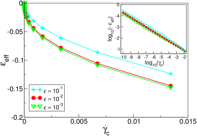
Figure 3: Mapping a compression melted glassy state onto an effective fluid state obtained by matching the low shear viscosity. The effective distance to the glass transition $\varepsilon_{\text{eff}}$ is shown as a function of the compressional rate $\dot{\gamma}_{c}$, for different values of $\varepsilon$. The points are numerical data and the lines provide a guide for the eye. The inset shows the same data on a logarithmic scale.

The above findings are in good qualitative agreement with the experimental results obtained in [Ovarlez et al. (2010)] (cf. Fig.3 therein). In order to characterize more precisely the flow curves at finite $\dot{\gamma}_{c}$ we show in Fig.2 the low shear viscosity $\eta=\sigma_{xy}/\dot{\gamma}_{s}$, scaled by the yield stress $\sigma_{\text{yield}}$, as a function of $\dot{\gamma}_{c}$ for three different positive values of $\varepsilon$. For $\dot{\gamma}_{c}<10^{-5}$ we find very good data collapse onto a master curve. For $\dot{\gamma}_{c}>10^{-4}$ clear deviations from universality set in, signifying that the compression induced structural relaxation processes are occurring on a timescale within the microscopic regime, for which $\eta$ becomes an $\varepsilon$ independent quantity (around $\dot{\gamma}_{s}=10^{-4}$ for the parameter set used in Fig.1). Provided that $\dot{\gamma}_{c}<\tau_{\beta}^{-1}$ we find that the numerical data are well represented by the power-law scaling

$$\eta/\sigma_{\text{yield}}=A\dot{\gamma}_{c}^{\alpha}\,,$$ (19)

with $\alpha=-1$, in agreement with the experimental findings of Ovarlez et al. (2010). The constant of proportionality $A$ is independent of $\varepsilon$ (both $\eta$ and $\sigma_{\text{yield}}$ vary in the same way with this parameter). Given the lack of detailed material specificity in the schematic model, we are led to believe that $\alpha=-1$ is a universal exponent, independent of both the details of the material under consideration and of the precise nature of the primary and perturbing flows. Our findings suggest that any constitutive theory capable of describing a three dimensional dynamic yield stress (‘yield stress surface’ [Brader et al. (2009)]) will inevitably recover the scaling (19) with $\alpha=-1$, when applied to tackle mixed flows. In particular, we anticipate that the full wavevector dependent mode-coupling constitutive equation [Brader et al. (2008)] would predict the same scaling behaviour, although this claim remains to be confirmed by explicit calculations. Within mode-coupling-based approaches the value of the scaling exponent $\alpha$ is a natural consequence of the way in which strain enters the memory function (8).

The flow curves presented in Fig.1 for various values of $\dot{\gamma}_{c}$ are very reminiscent of the (more familiar) flow curves either measured or calculated under simple shear with $\dot{\gamma}_{c}=0$ and $\varepsilon<0$, i.e. states which would remain fluid in the absence of flow (see, e.g. Fuchs and Cates (2003)). This similarity suggests that it may be possible to map, at least approximately, the shear response of a steadily compressed, glassy system with $\dot{\gamma}_{c}\neq 0$ and $\varepsilon>0$ onto an uncompressed, fluid system, $\dot{\gamma}_{c}=0$, at some effective, negative value of the separation parameter $\varepsilon_{\text{eff}}$. One possible way to realize such a mapping is to adjust $\varepsilon_{\text{eff}}$ for a given $\dot{\gamma}_{c}$ to obtain equal values for the low shear viscosity of the compressed glass and effective fluid systems. The results of performing this procedure for three values of $\varepsilon$ are shown in Fig.3. It should be noted that the mapping between $\varepsilon_{\text{eff}}$ and $\dot{\gamma}_{c}$ becomes discontinuous at $\dot{\gamma}_{c}=0$ at which point $\varepsilon_{\text{eff}}=\varepsilon>0$. The inset of Fig.3 shows the same data on a logarithmic scale. In this representation it becomes apparent that the data follow a power law

$$\varepsilon_{\text{eff}}\sim-\dot{\gamma}_{c}^{\beta}\,.$$ (20)

Fits to our numerical data yield values for the exponent $0.41<\beta<0.43$.

Within the quiescent $F_{12}$ schematic model [Götze (2008), Götze (1984)], to which the present theory reduces in the absence of flow, it is known that the zero shear viscosity exhibits a power law divergence as $\varepsilon$ approaches the glass transition from below

$$\eta\sim(-\varepsilon)^{-\delta}\,,$$ (21)

where $\delta$ is the same exponent as that describing the divergence of $\tau_{\alpha}$ at the glass transition. Note that the symbol $\delta$ is employed here for this exponent, rather than the standard choice $\gamma$, in order to avoid confusion with the strain. When employing the Percus-Yevick approximation to the static structure factor as input, the wavevector dependent mode-coupling theory predicts that for hard-spheres the viscosity exponent takes the value $\delta=2.46$ (identifying $\varepsilon$ as the volume fraction, relative to the transition point) [Götze and Sjögren (1992)]. Within the present schematic model we obtain $\delta=2.3$ (see also footnote footnote ). Given this information about the divergence of $\eta$ in the quiescent system, the power law relation for the mapping (20) is already implicit in the data shown in Fig.2. Using the relations (19) and (21) the relation (20) can be deduced, where the exponent $\beta$ is given by $\beta=\alpha/(-\delta)=0.43$, which is consistent with the results of our numerical fits.

V Analytic perturbative results

We have so far focused on the special case of mixed shear and compressional flows. For any given value of $\dot{\gamma}_{c}<\Gamma$ we have shown that there exists a Newtonian regime in the stress response to the shear flow, provided $\dot{\gamma}_{s}<\dot{\gamma}_{c}$ (see Fig.1) footnote2 . In this section, we now consider more general situations for which a second slow flow $\boldsymbol{\kappa}_{2}$ is added to a dominant flow $\boldsymbol{\kappa}_{1}$ (while keeping the requirements of incompressibility and homogeneity). In the present context a sufficient condition for the second flow to be considered ‘slow’ is that $\dot{\gamma}_{2}\ll\dot{\gamma}_{1}$, where the characteristic shear rates are now identified as $\dot{\gamma}_{i}=\sqrt{\boldsymbol{\kappa}_{i}\!:\!\boldsymbol{\kappa}^{T}_{i}}$ for $i=1,2$ (where ${\bf A}\!:\!{\bf B}\equiv\sum_{ij}A_{ij}B_{ji}$). In Subsections V.1-V.3, we provide perturbative constitutive equations for three different cases. In the first of these cases, we consider $\boldsymbol{\kappa}_{1}$ and $\boldsymbol{\kappa}_{2}$ as steady flows (without any other restriction), derivate the corresponding pertubative constitutive equation and finally apply this latter to our coupled compressional and shear flows, in order to theoretically account for the Newtonian viscous response to $\boldsymbol{\kappa}_{2}$ discussed in Sec. IV, and to finally make the connection with the phenomenological constitutive equation obtained by Ovarlez et al.. In the second case, we still consider steady flows, but this time with the additional requirement of ‘commutating’ flows, i.e. $[\boldsymbol{\kappa}_{1},\boldsymbol{\kappa}_{2}]\equiv\boldsymbol{\kappa}_{1}\cdot\boldsymbol{\kappa}_{2}-\boldsymbol{\kappa}_{2}\cdot\boldsymbol{\kappa}_{1}=0$, whereas in the third case $\boldsymbol{\kappa}_{2}$ is time-dependent and the requirement of commutating flows is maintained. We also illustrate these last two cases with instructive examples.

V.1 Newtonian viscous response

V.1.1 Perturbation expansion

The first point to note is that the isotropic modulus $G(t)$ decays on the timescale $\dot{\gamma}_{1}^{-1}$; the slower secondary flow has no influence on the structural relaxation. We henceforth make this fact explicit in the notation for the modulus by writing $G(t;\dot{\gamma}_{1},\dot{\gamma}_{2})\equiv G(t;\dot{\gamma}_{1})\equiv G_{1}(t)$. For steady flows the constitutive equation (5) may thus be simplified to

$$\boldsymbol{\sigma}=\int_{0}^{\infty}\!\!dt\left(\frac{\partial}{\partial t}\boldsymbol{B}(t)\right)G_{1}(t).$$ (22)

Although the modulus is essentially independent of $\dot{\gamma}_{2}$, the Finger tensor depends nonlinearly upon both $\boldsymbol{\kappa}_{1}$ and $\boldsymbol{\kappa}_{2}$. In order to address the case $\dot{\gamma}_{2}\ll\dot{\gamma}_{1}$ we expand the Finger tensor (4) to first order in $\boldsymbol{\kappa}_{2}$. For the mixed flow under consideration $\boldsymbol{B}(t)$ is given by

$$\boldsymbol{B}(t)=e^{(\boldsymbol{\kappa}_{1}+\boldsymbol{\kappa}_{2})t}e^{(\boldsymbol{\kappa}^{T}_{1}+\boldsymbol{\kappa}^{T}_{2})t}.$$ (23)

The desired partial linearization of (23) with respect to $\boldsymbol{\kappa}_{2}$ is complicated by the fact that the two velocity gradient tensors do not necessarily commute.

In order to proceed we consider the following Taylor expansion

$$e^{\hat{x}+\alpha\hat{y}}=e^{\hat{x}}+\alpha\left[\frac{d}{d\alpha}e^{\hat{x}+\alpha\hat{y}}\right]_{\alpha=0}\!+\;\mathcal{O}(\alpha^{2}),$$ (24)

where $\hat{x}$ and $\hat{y}$ are arbitrary operators independent of the scalar coupling parameter $\alpha$. The derivative may be obtained using the Feynman identity [Feynman (1951)]

$$\left[\frac{d}{d\alpha}e^{\hat{x}+\alpha\hat{y}}\right]_{\alpha=0}=\int_{0}^{1}\!d\lambda\,e^{\hat{x}(1-\lambda)}\hat{y}\,e^{\hat{x}\lambda}.$$ (25)

Applying (24) and (25) to (23) we obtain the leading order result

$$\boldsymbol{B}(t)=\boldsymbol{B}_{1}(t)+\int_{0}^{t}\!\!ds\,\left(\boldsymbol{U}(t,s)+\boldsymbol{U}^{T}(t,s)\right),$$ (26)

where we define the following tensors

$$\boldsymbol{B}_{1}(t) \equiv \boldsymbol{E}_{1}(t)\!\cdot\!\boldsymbol{E}^{T}_{1}(t)$$ (27)

$$\boldsymbol{U}(t,s) \equiv \boldsymbol{E}_{1}(t)\!\cdot\!\boldsymbol{E}_{1}(-s)\!\cdot\!\boldsymbol{\kappa}_{2}\!\cdot\!\boldsymbol{E}_{1}(s)\!\cdot\!\boldsymbol{E}^{T}_{1}(t),$$ (28)

where $\boldsymbol{E}_{1}(t)=\exp(\boldsymbol{\kappa}_{1}t)$. Eq.(26) is linear in $\boldsymbol{\kappa}_{2}$ but retains all orders of the dominant flow $\boldsymbol{\kappa}_{1}$. Substitution of (26) into (22) thus yields a stress tensor consisting of two terms,

$$\boldsymbol{\sigma} = \int_{0}^{\infty}\!\!\!\!dt\,\left(\frac{\partial}{\partial t}\boldsymbol{B}_{1}(t)\right)G_{1}(t)$$ (29)

$$+\int_{0}^{\infty}\!\!\!\!dt\frac{\partial}{\partial t}\left[\int_{0}^{t}\!\!ds\,\left(\boldsymbol{U}(t,s)+\boldsymbol{U}^{T}(t,s)\right)\right]G_{1}(t)$$

$$\equiv \boldsymbol{\sigma}_{1}+\delta\boldsymbol{\sigma}\quad,$$

where $\boldsymbol{\sigma}_{1}$ is the stress arising purely from the dominant flow and $\delta\boldsymbol{\sigma}$ is the additional contribution from the slow perturbation.

The perturbative term $\delta\boldsymbol{\sigma}$ in (29) is a tensor whose elements depend upon time as $[\cdot]_{ij}\sim t^{n_{ij}}$, where $n_{ij}\geq 1$ is an integer. Within the schematic model the relaxation time determining the decay of $G_{1}(t)$ is given by $\tau_{\alpha}=\gamma_{\rm cr}/\dot{\gamma}_{1}$, where $\gamma_{\rm cr}$ is the cross-over strain parameter entering (9). This decay serves to cut off the integral in (29) at the upper limit $t\sim\tau_{\alpha}$, with the consequence that the numerically largest elements of $[\cdot]_{ij}$ arising from terms with $n_{ij}=1$ are $\mathcal{O}(\eta_{1}\gamma_{\rm cr})$. In a (repulsive) colloidal glass any given colloid is trapped within a cage of nearest neighbours. The cross-over strain parameter $\gamma_{\rm cr}$ is related to the strain at which the cages begin to be broken by the external flow. Typical values for this dimensionless parameter from simulation or experiment are $\gamma_{\rm cr}\approx 0.1$ [Zausch et al. (2008)].

We now apply the perturbative formula (29) to the coupled compressional and shear flows expressed by the matrices (11), with $\boldsymbol{\kappa}_{1}=\boldsymbol{\kappa}_{c}$ and $\boldsymbol{\kappa}_{2}=\boldsymbol{\kappa}_{s}$. Since no complete analytic expression is known for the density correlator $\Phi$, we approximate the modulus $G_{1}(t)$ by an exponentially decaying function $G_{1}(t)\approx G_{\infty}\exp(-\dot{\gamma}_{1}t/\gamma_{\rm cr})$, where $G_{\infty}$ is a constant. Under this approximation, Eq. (29) becomes

$$\boldsymbol{\sigma} = \eta_{1}\dot{\gamma}_{c}\left(\begin{array}[]{ccc}\frac{1}{1-\gamma_{cr}}&0&0\\ 0&\frac{-2}{1+2\gamma_{cr}}&0\\ 0&0&\frac{1}{1-\gamma_{cr}}\end{array}\right)$$ (33)

$$+2\frac{2\eta_{1}}{(2+5\gamma_{cr}+2\gamma_{cr}^{2})}\boldsymbol{D}_{2}\quad,$$ (34)

where $\eta_{1}\equiv\int_{0}^{\infty}dt\,\,G_{1}(t)$ is the rate dependent shear viscosity of the primary flow alone and $\boldsymbol{D}_{2}\equiv(\boldsymbol{\kappa}_{2}+\boldsymbol{\kappa}^{T}_{2})/2$ is the symmetric part of the velocity gradient matrix $\boldsymbol{\kappa}_{2}$. The second term in (34) is nothing but the expression of a Newtonian-type viscous response to the secondary flow $\boldsymbol{\kappa}_{2}$ (shear flow) with a viscosity mainly determined by the strain rate of the dominant flow $\dot{\gamma}_{1}$ (compressional rate) through $\eta_{1}$. This is in agreement with what we numerically showed in Sec. IV.

V.1.2 Empirical constitutive equation

In [Ovarlez et al. (2010)], Ovarlez et al. proposed an empirical constitutive equation to account for the viscous stress measured in a number of fluidized glassy systems. In the notation of the present work the proposed constitutive relation is

$$\boldsymbol{\sigma}=2\left[\frac{\sigma_{\rm yield}+kd^{n}}{d}\right]\boldsymbol{D},$$ (35)

where $k$ and $n$ are scalar parameters and $d\equiv\sqrt{2\boldsymbol{D}\!:\!\boldsymbol{D}}$ is an invariant of the symmetric part of the total velocity gradient $\boldsymbol{D}=(\boldsymbol{\kappa}+\boldsymbol{\kappa}^{T})/2$. The isotropic viscosity appearing in square parentheses in (35) is obtained from a straightforward generalization of the familiar scalar Hershel-Bulkley law for the shear stress, $\sigma_{\rm sh}=({\sigma_{\rm yield}}+k\dot{\gamma}^{n})$.

If we neglect the cross-over strain parameter $\gamma_{cr}$ (whose value is already small, $\gamma_{cr}\approx 0.1$), then the second term in our perturbative constitutive equation (34) becomes $\delta\boldsymbol{\sigma}=2\eta_{1}\boldsymbol{D}_{2}$, which is entirely consistent with the implicit second term in the empirical relation (35). Indeed, for $\dot{\gamma}_{1}\gg\dot{\gamma}_{2}$ the generalized Hershel-Bulkley effective viscosity $(\sigma_{\rm yield}+kd^{n})/d$ is dominated by the fastest flow and is effectively independent of $\dot{\gamma}_{2}$. We can thus make the following correspondence between viscosities appearing in the schematic (34) and empirical (35) constitutive equations

$$\eta_{1}\equiv\int_{0}^{\infty}\!\!dt\,G_{1}(t)\;\Longleftrightarrow\;\frac{\sigma_{\rm yield}+kd^{n}}{d}.$$ (36)

The linear dependence of $\boldsymbol{D}$ on the velocity gradient tensor thus enables (35) to be rewritten as

$$\boldsymbol{\sigma}=\boldsymbol{\sigma}_{1}+2\eta_{1}\boldsymbol{D}_{2},$$ (37)

thus making explicit the connection between (34) and (35).

V.2 Anisotropic viscosity

We still consider steady flows $\boldsymbol{\kappa}_{1}$ (dominant flow) and $\boldsymbol{\kappa}_{2}$ (secondary flow), but now with the restriction of commutating flows, i.e. $\left[\boldsymbol{\kappa}_{1},\boldsymbol{\kappa}_{2}\right]=0$. Such flows have the property that the total deformation tensor can be formed from the product of the individual deformations, $\boldsymbol{E}(t)=\boldsymbol{E}_{1}(t)\boldsymbol{E}_{2}(t)$. As we will see, this restriction allows for more tractable pertubative constitutive equations.

With $\left[\boldsymbol{\kappa}_{1},\boldsymbol{\kappa}_{2}\right]=0$, the expression (26) then reduces to

$$\boldsymbol{B}(t)=\boldsymbol{B}_{1}(t)\,+\;2t\,\boldsymbol{E}_{1}(t)\!\cdot\!\boldsymbol{D}_{2}\!\cdot\!\boldsymbol{E}_{1}^{T}(t)\quad.$$ (38)

Substitution of (38) into (22) yields the following form for the stress tensor

$$\boldsymbol{\sigma} = \boldsymbol{\sigma}_{1}+2\eta_{1}\boldsymbol{D}_{2}$$

$$+\,2\!\int_{0}^{\infty}\!\!\!\!dt\,G_{1}(t)\left[\frac{\partial}{\partial t}\left(t\,\boldsymbol{E}_{1}(t)\!\cdot\!\boldsymbol{D}_{2}\!\cdot\!\boldsymbol{E}_{1}^{T}(t)\right)\!-\boldsymbol{D}_{2}\right].$$

The anisotropic third term in (V.2) is the result of a nonlinear operator acting on the perturbing velocity gradient $\boldsymbol{D}_{2}$ and incorporates information about the symmetry imposed on the system by the dominant fluidizing flow.

For incompressible isotropic fluids in the Newtonian regime the viscosity in any given flow can be determined from the shear viscosity via Trouton’s rules (e.g. $\eta_{\rm el}=3\eta_{\rm sh}$, where $\eta_{\rm el}$ is the elongational viscosity in uniaxial extension). Trouton’s rules no longer hold in the present case, due to the presence of the third term in (V.2).

In order to explicitly demonstrate the relative magnitude of the anisotropy, we consider the special case of perpendicular shear flow $(\boldsymbol{\kappa}_{1})_{ij}=\dot{\gamma}_{1}\delta_{ix}\delta_{jy}$, $(\boldsymbol{\kappa}_{2})_{ij}=\dot{\gamma}_{2}\delta_{iz}\delta_{jy}$ and again approximate the modulus by an exponentially decaying function $G_{1}(t)\approx G_{\infty}\exp(-\dot{\gamma}_{1}t/\gamma_{\rm cr})$. Under this simplifying assumption Eq.(V.2) becomes

$$\boldsymbol{\sigma}=\boldsymbol{\sigma}_{1}+2\eta_{1}\dot{\gamma}_{2}\!\left(\begin{array}[]{ccc}0&0&0\\ 0&0&1/2\\ 0&1/2&0\\ \end{array}\right)\!+2\eta_{1}\dot{\gamma}_{2}\!\left(\begin{array}[]{ccc}0&0&\gamma_{\rm cr}\\ 0&0&0\\ \gamma_{\rm cr}&0&0\\ \end{array}\right)\!.$$ (46)

(47)

The small off-diagonal elements which appear in the third term of (47) are generated by the coupling between primary and perturbing flows and may be viewed as a correction, at around the $10$% level, to the dominant isotropic viscosity $\eta_{1}$. The appearance of these additional contributions to the viscous stress can be attributed to the normal stress differences generated by the primary flow. Constitutive theories with vanishing normal stress differences will always predict an isotropic viscous response to perturbing flows.

It is interesting to note that the stress tensor (V.2) may be formally expressed in terms of an anisotropic viscosity

$$(\boldsymbol{\sigma})_{ij}=(\boldsymbol{\sigma}_{1})_{ij}\;+\;2(\boldsymbol{\eta})_{ijkl}(\boldsymbol{D}_{2})_{kl},$$ (48)

where the fourth rank tensor $\boldsymbol{\eta}$ with components $(\boldsymbol{\eta})_{ijkl}$ is given in terms of the shear modulus and the deformation gradient of the dominant flow

$$(\boldsymbol{\eta})_{ijkl}=2\!\int_{0}^{\infty}\!\!\!\!dt\,G_{1}(t)\left[\frac{\partial}{\partial t}t\,(\boldsymbol{E}_{1}(t))_{ik}(\boldsymbol{E}_{1}(t))_{jl}\right].$$ (49)

If the dominant flow is switched off, then $\boldsymbol{E}_{1}(t)=\boldsymbol{1}$ and (49) reduces to the familiar isotropic viscosity $\eta_{ijkl}=2\eta_{0}\delta_{ik}\delta_{jl}$, where $\eta_{0}$ is the zero shear viscosity (infinite for glassy states with $\varepsilon>0$). Given that the dominant flow fixes the anisotropy of the system it is not surprising that the viscosity experienced by the perturbing flow is a tensorial quantity.

Finally, we note that the presence of anisotropy prevents a general three dimensional mapping of a flow fluidized glass onto an effective fluid state with $\varepsilon<0$, as performed for the special case of mixed compressional and shear flow in Sec. IV.

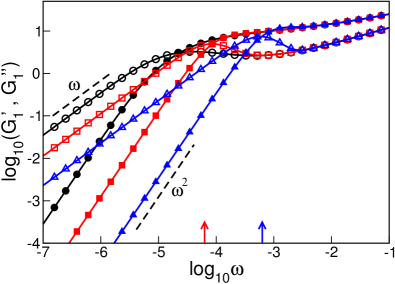
Figure 4: The othogonal superposition storage ($G_{1}^{\prime}$, filled symbols) and loss ($G_{1}^{\prime\prime}$, open symbols) moduli as a function of frequency for a fluid state. The (black) circles show the standard linear response moduli calculated at a vanishing steady shear rate $\dot{\gamma}_{1}=0$. The (red) squares and (blue) triangles show the moduli calculated at finite steady shear rates, $\dot{\gamma}_{1}=10^{-5}$ and $10^{-4}$, respectively. The arrows indicate the characteristic frequency $2\pi\dot{\gamma}_{1}$ below which the structural relaxation is dominated by the steady shear (which coincides approximately with the crossing point of the moduli). Parameter set $(\Gamma=1,\nu_{\sigma}=100,\gamma_{\rm cr}=1,\nu=1,\varepsilon=-5\times 10^{-3})$.

V.3 Superposition spectroscopy

A special case of mixed flow which has received some attention in the rheological literature is small amplitude oscillation superposed onto steady shear. Largely due to constraints imposed by the available apparatus, the majority of the experimental works have involved parallel shearing flows using either cone-plate [Booij (1966), Osaka et al. (1965)] or Couette [Vermant et al. (1998)] rheometers. The measured viscoelastic parallel superposition moduli depend upon both the microstructure under steady shear and its evolution with changes in shear rate.

A more informative, albeit harder to realize, mixed flow consists of oscillatory shear superposed perpendicular to the main flow direction. The orthogonality of the flows makes possible a mechanical spectroscopy of flowing systems which can probe flow induced changes in the microstructure and which may be used as a useful test of constitutive equations [De Cleyn and Mewis (1987), Kwon and Leonov (1993), Leonov et al. (1976), Tanner and Simmons (1967)]. For details on the experimental realization of such orthogonal flows we refer the reader to Vermant et al. (1997).

As a specific example of orthogonal oscillation we consider the mixed flow

$$(\boldsymbol{\kappa}_{1})_{ij} = \dot{\gamma}_{1}\delta_{ix}\delta_{jy}$$ (50)

$$(\boldsymbol{\kappa}_{2})_{ij} = \gamma_{0}\,\omega\cos(\omega t)\delta_{iz}\delta_{jy},$$ (51)

where $\omega$ is the angular frequency and $\gamma_{0}$ is the amplitude of the oscillatory strain (assumed to be small). The time-dependence of the perturbing flow $\boldsymbol{\kappa}_{2}$ requires us to use a time-ordered exponential to express the corresponding deformation tensor, namely

$$\boldsymbol{E}_{2}(t,t^{\prime})=e_{+}^{\int_{t^{\prime}}^{t}ds\boldsymbol{\kappa}_{2}(s)}\quad,$$ (52)

where the exponential is defined according to

$$e_{+}^{\int_{t^{\prime}}^{t}\!dsA(s)}=\boldsymbol{1}+\int_{t^{\prime}}^{t}\!\!\!dsA(s)+\int_{t^{\prime}}^{t}ds_{1}\int_{t^{\prime}}^{s_{1}}\!\!\!ds_{2}\,\,A(s_{1})A(s_{2})+\ldots$$ (53)

We also require the time-dependent expression for the stress tensor given by (5). After linearization with respect to $\boldsymbol{\kappa}_{2}$ and making use of $\left[\boldsymbol{\kappa}_{1},\boldsymbol{\kappa}_{2}\right]=0$, we obtain a formula for the stress tensor analogous to (V.2),

$$\boldsymbol{\sigma}(t) =\boldsymbol{\sigma}_{1}+\int_{-\infty}^{t}\!\!\!\!\!\!dt^{\prime}G_{1}(t,t^{\prime};\dot{\gamma}_{1})$$

$$\times\left\{-\frac{\partial}{\partial t^{\prime}}\left[\boldsymbol{E}_{1}(t-t^{\prime})\!\cdot\!\left(\int_{t^{\prime}}^{t}\!\!\!\!ds\,\,2\,\,\boldsymbol{D}_{2}(s)\right)\!\cdot\!\boldsymbol{E}_{1}^{T}(t-t^{\prime})\right]\right\}.$$

Substituting (50) and (51) into (LABEL:stress_expansion_time) and making use of standard trigonometric addition formulas yields

$$\sigma_{zy}(t)\!=\!\gamma_{0}G^{\prime}_{1}(\omega;\dot{\gamma}_{1})\sin(\omega t)+\gamma_{0}G^{\prime\prime}_{1}(\omega;\dot{\gamma}_{1})\cos(\omega t),$$

(55)

where the orthogonal superposition moduli are given by

$$G^{\prime}_{1}(\omega;\dot{\gamma}_{1}) = \omega\!\int_{0}^{\infty}\!\!dt^{\prime}\sin(\omega t^{\prime})\,G_{1}(t^{\prime};\dot{\gamma}_{1}),$$ (56)

$$G^{\prime\prime}_{1}(\omega;\dot{\gamma}_{1}) = \omega\!\int_{0}^{\infty}\!\!dt^{\prime}\cos(\omega t^{\prime})\,G_{1}(t^{\prime};\dot{\gamma}_{1}).$$ (57)

In Eqs.(55-57) we have made explicit the dependence of the moduli upon the steady shear rate $\dot{\gamma}_{1}$. The application of oscillations perpendicular to the flow thus enable the modulus under steady shear to be investigated and provide information about the shear induced relaxation of stress fluctuations. We note that identical moduli (56) and (57) would be obtained had we chosen the alternative perturbing flow $(\boldsymbol{\kappa}_{2})_{ij}=\gamma_{0}\,\omega\cos(\omega t)\delta_{ix}\delta_{jz}$ and determined the stress component $\sigma_{xz}$.

In Fig.4 we show the orthogonal superposition moduli as a function of frequency for three different values of the steady shear rate $\dot{\gamma}_{1}$. For $\dot{\gamma}_{1}=0$ we recover the standard linear response moduli, for which the viscous loss dominates the elastic storage for frequencies less than $2\pi/\tau_{\alpha}$. For the fluid state considered $\tau_{\alpha}$ is finite ($\varepsilon<0$). As the steady shear rate is increased, relaxation processes with rates less than $\dot{\gamma}_{1}$ are suppressed and the point at which the storage and loss moduli cross moves to higher frequency. These findings are consistent with the experimental results of both Booij (1966) and Vermant et al. (1998). The underlying physics here is essentially the same as that leading to the shift of the Newtonian regime shown in Fig.1. At low frequencies the orthogonal superposition moduli retain the same frequency scaling as in the familiar unsheared situation, namely $G^{\prime}_{1}\sim\omega^{2}$ and $G^{\prime\prime}_{1}\sim\omega$. We note also that the Kramers-Kronig relations remain valid for finite values of $\dot{\gamma}_{1}$.

In addition to the speeding up of structural relaxation induced by the steady shear, the loss modulus also displays a more pronounced $\alpha$-peak compared to the unsheared function. This feature is related to the functional form of the $\alpha$-decay of the transient density correlator. In the absence of shear $\Phi(t)$ decays as a stretched exponential, whereas under shear the final decay is closer to pure exponential. However, it is likely that more accurate (i.e. beyond schematic) orthogonal moduli, obtained either from experiment or more detailed microscopic calculations/simulations, would differ qualitatively in the region of the $\alpha$-peak. There is accumulating evidence [Zausch et al. (2008)] that $G_{1}(t;\dot{\gamma}_{1})$ becomes negative at long times and, as this feature is not captured by the simple schematic model employed here, differences in the Fourier transformed quantity around $\omega=2\pi\dot{\gamma}_{1}$ may be anticipated. The negative tail of $G_{1}(t;\dot{\gamma}_{1})$ is related to the existence of a maximum in the shear stress as a function of time following the onset of steady shear [Zausch et al. (2008)]. The ‘stress overshoot’ is present in the full wavevector dependent mode-coupling equations [Brader et al. (2008)] but gets lost in simplifying the theory to the schematic level.

VI Discussion and conclusions

In this paper we have demonstrated that the MCT-based schematic model of Brader et al. (2009) can qualitatively account for the experimental results on three dimensional flow of soft glassy materials reported in [Ovarlez et al. (2010)]. In particular, the competition of timescales which arises from applying flows of differing rate appears to be correctly incorporated into the model. The main outcome of our analysis is that the viscous response to a perturbing secondary flow is dominated by the primary flow rate. Although subtle anisotropic corrections to this picture do emerge from our equations, it remains to be seen whether these have significant consequences for experiments in any particular rheometer geometry.

A key feature of the mode-coupling constitutive theory is that it captures the transition from an ergodic fluid to an arrested glass as a function of the coupling strength. The present study demonstrates that the theory qualitatively accounts for experimental data on mechanically fluidized glassy systems in three dimensional situations. What remains to be established is whether the experimental yield surface of a colloidal glass agrees with the (almost) von Mises form [Hill (1971)] predicted by the schematic model [Brader et al. (2009)]. A true measurement of the yield surface would require a rheometer which enables parameterization of the entire family of velocity gradients, incorporating both uniaxial and planar extensional flows. This has not yet been achieved. Given the very different mechanisms underlying plastic flow in colloidal glasses and metals (for which the von Mises yield surface was originally proposed) direct measurements of the yield surface could prove very informative.

The good qualitative agreement of our theory with the experimental results of Ovarlez et al. (2010) on fluidized glasses is perhaps all the more surprising when recalling that the theory is constructed specifically for dispersions of spherical colloidal particles (without hydrodynamic interactions), whereas the experiments were performed on large aspect ratio Bentonite clay, a Carbopol gel and an emulsion. The consistent phenomenology presented by these disparate systems would seem to indicate that the sufficient elements required for a successful theory are (i) a well-founded geometrical structure (in the sense that its tensorial structure is appropriate), (ii) correct incorporation of flow induced relaxation rates. The specific nature of the interparticle interactions does not seem to be of particular importance, although we note that certain interaction potentials may be more susceptible to inhomogeneous flow (e.g. shear banding instabilities) than others. The presence of a spatially varying velocity gradient tensor $\boldsymbol{\kappa}$ would conflict with the assumption of translational invariance underlying our constitutive equation.

For the case of superposed compression and shear flow we have found that the viscosity felt by the perturbing shear flow is given by $2\eta_{1}/((2+5\gamma_{cr}+2\gamma_{cr}^{2}))$, which for the typical value $\gamma_{cr}\!=\!0.1$ is around $20$% less than the primary viscosity $\eta_{1}$. In [Ovarlez et al. (2010)] the sedimentation velocity of a sphere falling in the vorticity direction of a shear fluidized glass was observed to be a factor of $1.4$ larger than one would expect from a sphere falling through a fluid of viscosity $\eta_{1}$. Ovarlez et al. attributed this to hydrodynamic interactions between sedimenting particles. Although the flow around a falling sphere in shear flow is more complicated than the flows considered in the present work, it is nevertheless tempting to speculate that enhanced sedimentation velocity could be connected to a reduced effective viscosity, as occurs in (34), arising from a nontrivial coupling of the superposed flows. We leave a detailed application of our constitutive equation to the problem of sedimentation under shear to future work.

An aspect of the present work which may warrant further investigation is the possible analogy between systems with isotropic interparticle interactions, upon which anisotropy is imposed by external mechanical force fields, and intrinsically anisotropic materials such as liquid crystals [de Gennes and Prost (1993), Larson (1988)]. The theory of anisotropic fluids has a long history, beginning essentially with the work of Oseen in the 1930s [Oseen (1933)] and developed through the work of Ericksen (1959) and Leslie (1968). In all of these theoretical developments the anisotropy of the viscous response originates from the underlying anisotropy of the constituents; usually oriented polymers or rod-like particles with liquid crystalline order. Take the nematic phase as an example. Within a continuum mechanics description the orientational order is characterized by the director ${\bf n}$. In certain systems the director may be held fixed by the application of a suitably strong external field, in others it interacts with the imposed flow in a more complicated way. Either way, the presence of a preferred direction in the sample gives rise to an anisotropic viscous response (characterized e.g. by the five scalar Leslie viscosity coefficients). In the present case the anisotropy of the perturbation response is determined by the geometry of the primary flow. It may thus be anticipated that the eigenvectors of the primary deformation may play a role in the present theory analogous to that of ${\bf n}$ in the dynamics of nematics.

Throughout the present work we have focussed on the response of a glass which has already been fluidized by a primary flow of constant rate. However, within the same formalism we can also consider the predictions of our constitutive equation for the elastic response of a colloidal glass which has been pre-strained by a primary deformation at some point in the past (see the Appendix for more details on this point). For example, a colloidal glass subject to a shear strain below the yield strain may reasonably be expected to possess an anisotropic elastic response to an additional small perturbing strain (see (61) for verification of this assertion). Taking this idea a step further, it would be of interest to investigate the nature of the yield stress surface in such pre-strained glasses. Although both the topology of the surface and its invariance with respect to hydrostatic pressure will remain unchanged by pre-straining, significant deviations from circularity (over and above those already arising from normal stresses) can be envisaged. In reality these deviations may well be nonstationary, decaying away as the sample ages, but such subtle dynamic effects are beyond current formulations of the mode-coupling theory.

Acknowledgements

The authors thank M. E. Cates, M. Fuchs and Th. Voigtmann for comments on the manuscript. Funding was provided by the Swiss National Science Foundation.

Anisotropic elasticity

Integrating (5) by parts yields the following form for the schematic constitutive equation

$$\boldsymbol{\sigma}(t)= \boldsymbol{B}(t,-\infty)G(t,-\infty)-\nu_{\sigma}\boldsymbol{1}$$ (58)

$$\hskip 14.22636pt+\int_{-\infty}^{t}\!\!\!dt^{\prime}\,\boldsymbol{B}(t,t^{\prime})\frac{\partial}{\partial t^{\prime}}G(t,t^{\prime}).$$

For glassy states the modulus relaxes to a plateau value for long times and the contribution of the integral term to the overall numerical value of the stress is limited to a negligible integration over the $\beta$ relaxation (beyond this time the time derivative vanishes). The integral term may therefore be neglected to a good level of approximation.

We first consider the situation when the system is subjected to a mixed strain field $\boldsymbol{\epsilon}=\boldsymbol{\epsilon}_{1}+\boldsymbol{\epsilon}_{2}$, where $\boldsymbol{\epsilon}_{i}=(\nabla_{i}\boldsymbol{r}_{i}+\boldsymbol{r}_{i}\nabla_{i})$ is the infinitessimal strain due to flow $i$. Both of these strains are sufficiently small that the system remains in the purely elastic regime. The stress for long times after the application of the two strains is given by a simple linear superposition of the two elastic responses

$$\boldsymbol{\sigma}=2G_{\infty}\boldsymbol{\epsilon}_{1}+2G_{\infty}\boldsymbol{\epsilon}_{2},$$ (59)

as is expected from the linear theory of isotropic elasticity [Landau and Lifshitz (1986)]. Note that in (59) we have suppressed an irrelevant isotropic contribution $-\nu_{\sigma}\boldsymbol{1}$ (the system is incompressible).

We next consider the situation whereby $\boldsymbol{\epsilon}_{2}$ remains small but the strain due to the primary flow is allowed to be sufficiently large that some plastic rearrangements are induced. We nevertheless require that the total strain must still remain sufficiently small that the yield stress is not exceeded and the system remains solid. The analysis of this case neccessitates use of the partial expansion (38). We assume that the primary strain has been applied at some time in the distant past and that all plastic rearrangements have ceased by the time we apply the perturbing strain $\boldsymbol{\epsilon}_{2}$. The Finger tensor $\boldsymbol{B}_{1}(t)\equiv\boldsymbol{B}_{1}$ is thus independent of time at the present time $t$. For times $t$ following application of $\boldsymbol{\epsilon}_{2}$

$$\boldsymbol{\sigma}=\boldsymbol{\sigma}_{1}\,+\;2G_{\infty}\,\boldsymbol{E}_{1}\!\cdot\!\boldsymbol{\epsilon}_{2}\!\cdot\!\boldsymbol{E}_{1}^{T}.$$ (60)

By analogy with the situation considered in Sec. V.2, Eq.(60) can be expressed in terms of a fourth rank stiffness tensor

$$(\boldsymbol{\sigma})_{ij}=(\boldsymbol{\sigma}_{1})_{ij}+(\boldsymbol{C})_{ijkl}(\boldsymbol{\epsilon}_{2})_{kl}$$ (61)

where $(\boldsymbol{C})_{ijkl}=2G_{\infty}(\boldsymbol{E}_{1})_{ik}(\boldsymbol{E}_{1})_{jl}$. We note that the plateau value of the modulus $G_{\infty}$ may differ from its quiescent value as a result of plastic deformation occurring during or after application of the primary strain.

References

- (1) Banchio A.J., and J.F. Brady,“Accelerated Stokesian dynamics: Brownian motion” , J.Chem.Phys. 118, 10323-10332 (2003).
- (2) Besseling R., L. Isa, P. Ballesta, G. Petekidis, M.E. Cates, and W.C.K. Poon,“Shear Banding and Flow-Concentration Coupling in Colloidal Glasses”, Phys.Rev.Lett. 105, 268301 (2010).
- (3) Bird R.B., R.C. Armstrong, and O. Hassager, “Dynamics of Polymeric Liquids”, (Wiley, New York, 1987).
- (4) Booij H.C.,“Influence of superimposed steady shear flow on the dynamic properties of non-Newtonian fluids I. Measurements on non-Newtonian solutions”, Rheol.Acta 5, 215-221 (1966).
- (5) Brader J.M.,“Nonlinear rheology of colloidal dispersions”, J. Phys.: Condens. Matter 22, 363101 (2010).
- (6) Brader J.M.,“Solution of the Ornstein-Zernike Equation in the Critical Region”,International Journal of Thermophysics 27, 394-412 (2006).
- (7) Brader J.M., M. Siebenbürger, M. Ballauff, K. Reinheimer, M. Wilhelm, S. J. Frey, F. Weysser, and M. Fuchs,“Nonlinear response of dense colloidal suspensions under oscillatory shear: Mode-coupling theory and Fourier transform rheology experiments”, Phys.Rev.E 82, 061401 (2010).
- (8) Brader J.M., M.E. Cates, and M. Fuchs,“First-Principles Constitutive Equation for Suspension Rheology”, Phys. Rev. Lett. 101, 138301 (2008).
- (9) Brader J.M., Th. Voigtmann, M.E. Cates, and M. Fuchs,“Dense Colloidal Suspensions under Time-Dependent Shear”, Phys. Rev. Lett. 98, 058301 (2007).
- (10) Brader J.M., T. Voigtmann, M. Fuchs, R.G. Larson, and M.E. Cates,“Liquids and Structural Glasses Special Feature: Glass rheology: From mode-coupling theory to a dynamical yield criterion”, Proceedings of the National Academy of Sciences 106, 15186-15191 (2009).
- (11) De Cleyn G., and J. Mewis,“Constitutive equation for polymer liquids: application to shear flow”, J. Non-Newtonian Fluid Mech. 9, 91-105 (1987).
- (12) de Gennes P.-G., and J. Prost, “The Physics of Liquid Crystals” (Oxford University Press, 1993).
- (13) Dhont J.K.G., “An Introduction to the Dynamics of Colloids” (Amsterdam: Elsevier, 1996).
- (14) Doi M., and S.F. Edwards, “The Theory of Polymer Dynamics” (Oxford: Oxford University Press, 1989).
- (15) Ericksen J.L., “Anisotropic fluids”, Arch.Rat.Mech.Anal. 4, 231-237 (1959).
- (16) Feynman R.P.,“An Operator Calculus Having Applications in Quantum Electrodynamics”, Phys.Rev. 84, 108 (1951).
- (17) Frank M., D. Anderson, E.R. Weeks, and J.F. Morris,“Particle migration in pressure-driven flow of a Brownian suspension”, J.Fluid.Mech. 493, 363-378 (2003).
- (18) Fuchs M., High Solid Dispersions ed. M. Cloitre (Berlin: Springer, 2009).
- (19) Fuchs M., and M.E. Cates, “Theory of Nonlinear Rheology and Yielding of Dense Colloidal Suspensions”, Phys.Rev.Lett. 89, 248304 (2002).
- (20) Fuchs M. and M. Cates, “A mode coupling theory for Brownian particles in homogeneous steady flow”, J.Rheol. 53, 957-1000 (2009).
- (21) Fuchs M., and M.E. Cates,“Schematic models for dynamic yielding of sheared colloidal glasses ”, Faraday Discuss. 123, 267-286 (2003).
- (22) Götze W., “Complex Dynamics of Glass-Forming Liquids: A Mode-Coupling Theory” (Oxford University Press, Oxford, 2008).
- (23) Götze W., “Some aspects of phase transitions described by the self consistent current relaxation theory”, Z.Phys.B 56, 139-154 (1984).
- (24) Götze W., and L. Sjögren, “Relaxation processes in supercooled liquids”, Rep. Prog. Phys. 55, 241 (1992).
- (25) Henrich O., F. Weysser, M.E. Cates, and M. Fuchs, “Hard discs under steady shear: comparison of Brownian dynamics simulations and mode-coupling theory”, Phil.Trans.Roy.Soc.A 367, 5033-5050 (2009).
- (26) Hill R., “The Mathematical Theory of Plasticity” (Oxford University Press, 1971).
- (27) Krüger M., F. Weysser, and M. Fuchs, “Tagged-particle motion in glassy systems under shear: Comparison of mode coupling theory and Brownian Dynamics simulations.” Eur. Phys. J. E 34, 88 (2011)
- (28) Kwon Y., and A.I. Leonov, “Remarks on orthogonal superposition of small amplitude oscillations on steady shear flow”, Rheol.Acta 32, 108-112 (1993).
- (29) Landau L.D, and E.M. Lifshitz, “Theory of Elasticity” (Butterworths-Heinemann, 1986).
- (30) Larson R.G., “Constitutive Equations for Polymer Melts and Solutions” (Butterworths, London, 1988).
- (31) Leonov A.I., E.H. Lipkina, E.D. Paskhin, and A.N. Prokunin, “Theoretical and experimental investigation of shearing in elastic polymer liquids”, Rheol.Acta 15, 411-426 (1976).
- (32) Leslie F.M., “Some constitutive equations for liquid crystals”, Arch.Rat.Mech.Anal. 28, 265-283 (1968).
- (33) Mewis J., and N.J. Wagner, “Thixotropy”, Advances in Colloid and Interface Science 147-148, 214-227 (2009).
- (34) Osaka K., M. Tamura, M. Kurata and T. Kotaka, “Complex Modulus of Concentrated Polymer Solutions in Steady Shear1”, J.Phys.Chem. 69, 4183-4191 (1965).
- (35) Oseen C.W., “The theory of liquid crystals”, Trans.Faraday.Soc. 29, 883-899 (1933).
- (36) Ovarlez G., Q. Barral, and P. Coussot, “Three-dimensional jamming and flows of soft glassy materials ”, Nature materials 9, 115-119 (2010).
- (37) Tanner R.I, and J.M. Simmons, “Combined simple and sinusoidal shearing in elastic liquids”, Chem.Eng.Sci. 22, 1803-1815 (1967).
- (38) Vermant J., P. Moldenaers, J. Mewis, M. Ellis, and R. Garritano, “ Orthogonal superposition measurements using a rheometer equipped with a force rebalanced transducer ”, Rev.Sci.Instr. 68, 4090 (1997).
- (39) Vermant J., L. Walker, P. Moldenaers, and J. Mewis, “Orthogonal versus parallel superposition measurements ”, J. Non-Newtonian Fluid Mech. 79, 173-189 (1998).
- (40) Zausch J., J. Horbach, M. Laurati, S.U. Egelhaaf, J.M. Brader, Th. Voigtmann, and M, Fuchs, “From equilibrium to steady state: the transient dynamics of colloidal liquids under shear ”, J.Phys.Cond.Mat. 20, 404210 (2008).
- (41) The specific numerical value for the exponent from the schematic model depends upon the path chosen in the two-dimensional space of memory function coupling constants . By taking a standard linear path parameterized by (see text below Eq.(8)) we reproduce rather closely the viscosity divergence of the wavevector dependent theory for hard-spheres.
- (42) A completely analogous picture would have emerged, had we chosen a dominant shear flow with a perturbing compressional component. In this inverted thought experiment the dominant timescale would simply be set by .