Volovik effect in a highly anisotropic multiband superconductor: experiment and theory

Abstract

We present measurements of the specific heat coefficient $\gamma$($\equiv C/T)$ in the low temperature limit as a function of an applied magnetic field for the Fe-based superconductor BaFe₂(As_0.7P_0.3)₂. We find both a linear regime at higher fields and a limiting square root $H$ behavior at very low fields. The crossover from a Volovik-like $\sqrt{H}$ to a linear field dependence can be understood from a multiband calculation in the quasiclassical approximation assuming gaps with different momentum dependence on the hole- and electron-like Fermi surface sheets.

I Introduction

The symmetry and detailed structure of the gap function in the recently discovered iron pnictide Kamihara et al. (2008) and chalcogenide Hsu et al. (2008) high temperature superconductors is still under discussion. Across an increasingly numerous set of materials families, as well as within each family where superconductivity can be tuned by doping or pressure, experimental indications are that there is no universal gap structure. Wen (2011); [][;toappearinRev.Mod.Phys.(2011).]stewart11 Instead, the superconducting gap appears to be remarkably sensitive to details of the normal state properties. This “intrinsic sensitivity” Kemper et al. (2010) may be due to the unusual Fermi surface topology, consisting of small hole and electron pockets, and to the probable $A_{1g}$ symmetry of the superconducting gap which allows a continuous deformation of the order parameter structure from a fully gapped system to one with nodes (for a review see, e.g. Ref. Hirschfeld et al., 2011). It is important to keep in mind, though, that another possibility to account for the observed variability is that different experiments on the same material may probe selectively different Fermi surface regions and hence different gaps within the system.

The Ba-122 family of materials has been intensively studied because large high quality single crystals are relatively easy to produce. Stewart (2011); Kasahara et al. (2010) Within this family, the isovalently substituted system BaFe₂(As_1-xP_x)₂ with a maximum $T_{c}$ of 31 K is particularly intriguing because it exhibits a phase diagram and transport properties remarkably similar to the heterovalently doped system Ba(Fe_1-xCo_x)₂As₂ and displays many signatures of apparent quantum critical behavior at optimal doping. Kasahara et al. (2010); Jiang et al. (2009); Shishido et al. (2010) In the superconducting state, penetration depth, Hashimoto et al. (2010) NMR spin-lattice relaxation, Nakai et al. (2010) thermal conductivity temperature dependence, Hashimoto et al. (2010) and thermal conductivity angular field variation Yamashita et al. (2011) show clear indications of nodal behavior. Surprisingly, a linear field dependence of the specific heat Sommerfeld coefficient $\gamma$ was measuredKim et al. (2010) on optimally doped samples from the same batch. Such a behavior is expected for a fully gapped single band superconductor since the fermionic excitations from the normal cores of vortices provide the only contribution to $\gamma$ at low $T$, and the number of these vortices scales linearly with the field $H$. It was argued in Ref. Kim et al., 2010 that the specific heat measurement might be consistent with the other experiments suggesting nodes if the heavy hole sheets in the material were fully gapped, while the gaps on the lighter electron sheets were nodal. In such a case the $\gamma\sim\sqrt{H}$ behavior would be difficult to observe in experiment.

In this paper, we report new experimental data on the magnetic field dependence of the specific heat of optimally doped BaFe₂(As_1-xP_x)₂ samples. We have extended our previous measurements to 15 T to higher fields up to 35 T ($\approx\frac{2}{3}H_{c2}(0)$), where we find a continuation of the linear behavior reported earlier. However, more precise measurements at low fields have revealed the presence of a Volovik-like $\sqrt{H}$ term which persists roughly over a range of 4 T, crossing over to a linear behavior above this scale.  The observation of this term, consistent with nodes in the superconducting gap, therefore supports claims made in earlier work,Hashimoto et al. (2010); Nakai et al. (2010); Yamashita et al. (2011) without the need to assume an extremely large mass on the hole pockets.

Theoretical estimates using the Doppler shift method for isotropic gaps given in Ref. Bang, 2010 were oversimplified, but did show the need for a more thorough analysis of anisotropic multiband systems, and stimulated further experimental work, both of which we report here. The theoretical difficulties can be seen easily by considering a simple two-band model with two distinct gaps $\Delta_{1}$ and $\Delta_{2}$, where we assume for the moment that $\Delta_{2}>\Delta_{1}$. If the two bands are uncoupled, the two gaps correspond to two independent coherence lengths $\xi_{i}\simeq v_{F,i}/(\pi\Delta_{i})$, where $i=1,2$, and two independent “upper critical fields” $H_{c2,i}$. Vortex core states of the large gap $\Delta_{2}$ are confined to cores of radius $\sim\xi_{2}$. For fields in the range $H_{c2,1}\lesssim H\lesssim H_{c2,2}$, the vortex cores of the small gap will overlap, while the large gap cores will still be well separated. Note that if $\Delta_{1}$ is very small (these considerations also describe crudely nodal gaps), this field range can be wide and extend to quite low fields. On the other hand, methods of studying quasiparticle properties in superconductors are typically adapted to calculating near $H_{c1}$ or $H_{c2}$, i.e. in the limit of widely separated or nearly overlapping vortices. The current problem apparently contains elements of both situations. In the absence of interband coupling, of course, one can use different methods, corresponding to the appropriate field regimes, for the distinct bands. For coupled Fermi surfaces, however, such an approach is not viable. In the immediate vicinity of the transition, where the Ginzburg-Landau expansion is valid, there is a single length scale controlling the vortex structure. Kogan and Schmalian (2011) At low temperatures, where the measurements are carried out, however, the distinct length scales likely survive, although they are modified by the strength of the interband coupling, see below. Possible anisotropy of the gap on one or more Fermi surface sheets complicates the picture even further. We show here that judicious use of the quasiclassical approximation even with simplifying assumptions about the vortex structure can provide a general framework for the description of this problem, and a semiquantitative understanding of the new data on the BaFe₂(As_1-xP_x)₂ system. We compare our results with those obtained by Doppler-shift methods, and show that if properly implemented this method also gives reasonable qualitative results in the low field range.

This joint theory-experiment paper is organized as follows. We first present our experimental results on the BaFe₂(As_1-xP_x)₂ system in Section II and compare to our previous results, as well as to data by other groups on the related heterovalently doped Ba-122 materials. In Section III, we discuss the two-band quasiclassical model we use to study the system, and in Section IV we give our results. Finally in Section V we present our conclusions.

II Experimental

Tiny platelet crystals of BaFe₂(As_0.7P_0.3)₂ were prepared as described in Ref. Kasahara et al., 2010. Subsequent measurements on crystals extracted from various positions in the crucible using x-ray diffraction and energy dispersion (EDX) analysis give a phosphorous concentration of $32.9\pm 0.4\%$. A further test of the homogeneity of the crystals from a given growth batch is the measurement of the susceptibility at the superconducting transition as shown in Fig. 1 of Ref. Kim et al., 2010. Here, for a collage of $\sim 150$ mg of these crystals a rather narrow transition was observed. A collage of $18$ mg of these microcrystals was then mounted on a sapphire disk using GE7031 varnish. Approximately $75\%$ of the crystals had the magnetic field perpendicular to the a-b plane (the plane of the crystals), whereas the remaining crystals were randomly oriented. The sapphire disk was mounted in our time constant method calorimeter, Stewart (1983); *Andraka89 and the specific heat from $0.4$ to $7$ K in fields from $0$ to $35$ T was measured. Additionally, the specific heat of a standard (high purity Au) was measured in fields up to $14$ T. Results on the standard (not shown) indicate agreement with published values to within $\pm 3\%$ in all fields.

II.1 Results and Discussion

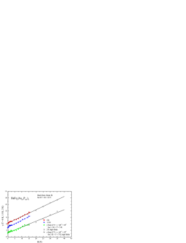
Figure 1: (Color online) The original specific heat dataKim et al. (2010) on BaFe₂(As_0.7P_0.3)₂ as a function of field up to 15 T (solid symbols) with data from present work between 15 T and 35 T (open symbols). Note the agreement between the linear, $C/T\propto H$, extrapolation of the 15 T (colored lines Kim et al. (2010)) and 35 T (black lines, present work) results. We extract $\gamma$ from the data using two (equivalent) methods: (a) by making an extrapolation $C/T=\gamma+\beta T^{2}+\delta T^{4}$ from 2 K and above or (b) by taking the value of $C/T$ at 1.5 and 2 K. The temperature restriction eliminates both the influence of the anomaly and the field-induced nuclear contribution (see text), negligible for $H\leq 4$ T above 1 K. The absolute accuracy of these data is $\pm 5\%$ while the precision of the data is approximately $\pm 2\%$. In addition, additional data with finer gradations in the measured fields up to $4$ T were taken to explore the low field non-linear behavior. These data are shown on an expanded scale in Fig. 2.

The specific heat coefficient $\gamma\equiv C/T$ of BaFe₂(As_0.7P_0.3)₂ for $0\leq H\leq 35$ T is shown by the open triangles in Fig. 1. There is a small low temperature anomaly in the specific heat data below about 1.4 K (discussed in detail in Kim et al., 2010). Such anomalies have been observed in other FePn samples, Kim et al. (2009) and in some cases, e.g. in BaFe_2-xCo_xAs₂, they show a rather strong magnetic field dependence. Kim et al. (2009) However, as discussed in our previous report Kim et al. (2010) of the data up to 15T, the anomaly in BaFe₂(As_0.7P_0.3)₂ is approximately field independent. Note that the small anomaly in the specific heat appears to vanish above 1.4 K, i.e. does not affect the estimate for $\gamma$ shown in Figs. 1 and 2 using data from 1.5 K and above.

In order to have a closer look at the low field dependence of the specific heat, these data are shown on an expanded scale in Fig. 2. In our analysis below, we focus on the asymptotic $T\rightarrow 0$ behavior since it is directly related to the density of states at the Fermi level, which is easy to calculate reliably, and since it gives essentially the same field dependence as the nonzero $T$ data.

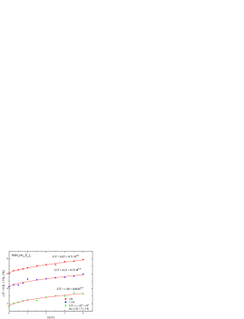
Figure 2: (Color online) Low field $\gamma$ data up to 4 T from Fig. 1 on an expanded scale for T=2 K (blue), 1.75 K (red) and 1.5 K (black symbols). Green symbols are asymptotic $\lim_{T\to 0}C/T$ determined over the range 1.5 K$<T<$5 K. The fitting functions of the data are labeled beside the curves. Best power law fits to field dependence are shown in each case.

III Model

III.1 Quasiclassical approximation

The quasiclassical (Eilenberger) approximation Eilenberger (1968); Larkin and Ovchinnikov (1969); Serene and Rainer (1983) is a powerful tool to describe the electronic properties of the superconducting state on the scales large compared to the lattice spacing, provided the condition $k_{F}\xi\gg 1$ is satisfied. Here $k_{F}$ is the Fermi momentum and $\xi$ the coherence length. Since in this limit we can think of quasiparticles as propagating coherently along a well-defined trajectory in real space, this method is particularly well suited to address the inhomogeneous situations, such as the vortex state of type-II superconductors (SCs). An alternative and frequently used approach to the vortex state is to take into account the (classical) shift of the quasiparticle energy due to the local supercurrent flow. Such an approximation, often referred to as the Doppler-shift approach, is valid for nodal SCs with considerable weight of extended quasiparticle excitations ouside the vortex cores. Using this method, Volovik showed that for superconductors with line nodes these extended quasiparticle excitations lead to a non-linear magnetic field dependence of the spatially averaged residual density of states $N(\omega=0,H)\propto N_{0}\sqrt{H/H_{c2}}$, the result known as the Volovik effect. Volovik (1993) This behavior was first confirmed by measurements of the specific heat Moler et al. (1997); Wang et al. (2001) and by subsequent calculations within the quasiclassical approximation for both a single vortex in a $d$-wave SC Ichioka et al. (1996); Schopohl and Maki (1995) and for a vortex lattice. Ichioka et al. (1997, 1999) Both quasiclassical and Doppler-shift methods fail at the lowest temperatures due to quantum effects Franz and Tevsanović (2000), but in known systems with $T_{c}\ll E_{F}$ these effects are negligible in practice. Both methods have successfully explained at a semiquantitative level the magnetic field dependence of the specific heat and thermal conductivity in a wide variety of unconventional superconductors. Vekhter and Vorontsov (2008) It was also shown that the accurately calculated quasiparticle excitation spectrum is consistent with STM studies of the electronic structure around a vortex core. Ichioka et al. (1997)

Many experimental techniques which are sensitive to the low-energy density of states, such as thermal conductivity, specific heat, and NMR relaxation rate, can be used to draw conclusions about the possible existence and the momentum dependence of quasiparticle excitation in the bulk of iron-based superconductors (FeSCs) and thus about the structure of the superconducting gap and the distribution of gap nodes. The low $T$ limit of the Sommerfeld coefficient in an applied magnetic field, $\gamma(H)$, is directly proportional to the spatially averaged local density of states (LDOS) at the Fermi level. The Doppler-shift method has been used to calculate the LDOS for a two-band SC with two isotropic gaps of unequal size $\Delta_{S}\neq\Delta_{L}$ and to give an interpretation of the experimental data available at that time.Bang (2010) However, the Doppler-shift approach cannot account properly for the contributions from the states in the vortex core that have a very large weight in the net DOS and hence gives a quantitatively and sometimes qualitatively inaccurate description of the electronic structure of the vortex. For example, in a simple $d$-wave superconductor the spatial tails of the low-energy density of states around the vortex are aligned in the wrong directions.Dahm et al. (2002) To obtain a quantitative fit to the specific heat data presented in the previous section and to allow for a more decisive conclusion about the gap structure of BaFe₂(As_0.7P_0.3)₂, we will therefore use the quasiclassical approximation, which we will briefly review in the following paragraphs.

In the quasiclassical method, the Gorkov Green’s functions are integrated with respect to the quasiparticle energy measured from the Fermi level. The normal and anomalous components $g(\mathbf{r},\theta,i\omega_{n})$ and $f(\mathbf{r},\theta,i\omega_{n})$ of the resulting propagator $\hat{g}$ obey the coupled Eilenberger equations

$$\left[2\left(i\omega_{n}+\frac{e}{c}\mathbf{v}_{F}\cdot\mathbf{A(r)}\right)+i\hbar\mathbf{v}_{F}\cdot\nabla\right]f(\mathbf{r},\theta,i\omega_{n})$$

$$\quad=2ig(\mathbf{r},\theta,i\omega_{n})\Delta(\mathbf{r},\theta),$$ (1a)

$$\left[2\left(i\omega_{n}+\frac{e}{c}\mathbf{v}_{F}\cdot\mathbf{A(r)}\right)-i\hbar\mathbf{v}_{F}\cdot\nabla\right]\bar{f}(\mathbf{r},\theta,i\omega_{n})$$

$$\quad=2ig(\mathbf{r},\theta,i\omega_{n})\Delta^{*}(\mathbf{r},\theta),$$ (1b)

that have to be complemented by the normalization condition

$$\hat{g}^{2}\equiv\begin{pmatrix}g&f\\ \bar{f}&-g\end{pmatrix}^{2}=\hat{1}\,.$$ (2)

Here $\Delta(\mathbf{r},\theta)$ is the order parameter, $\mathbf{A(r)}$ the vector potential, $\mathbf{v}_{F}$ is the Fermi velocity at the location at the Fermi surface labeled by $\theta$, and $\omega_{n}=(2n+1)\pi k_{B}T$ are the fermionic Matsubara frequencies. For two-dimensional cylindrical Fermi surfaces such as considered below, $\mathbf{v}_{F}=v_{F}\hat{\mathbf{k}}$ where $\hat{\mathbf{k}}=(\cos\theta,\sin\theta)$ and $\theta$ is the angle measured from the [100] direction. In that case it is natural to write the position vector in cylindrical coordinates, $\mathbf{r}=(\rho,\phi,z)$, where $\phi$ is the winding angle around the vortex in real space.

Making use of the symmetries Schopohl (1998) of the quasiclassical propagator

$$\bar{f}(\mathbf{r},\mathbf{k}_{F},i\omega_{n}) =f^{*}(\mathbf{r},\mathbf{k}_{F},-i\omega_{n}),$$ (3a)

$$f(\mathbf{r},-\mathbf{k}_{F},-i\omega_{n}) =f(\mathbf{r},\mathbf{k}_{F},i\omega_{n}),$$ (3b)

$$g(\mathbf{r},\mathbf{k}_{F},i\omega_{n}) =g^{*}(\mathbf{r},\mathbf{k}_{F},-i\omega_{n}),$$ (3c)

the diagonal part of the normalization condition (2) can be written in a more explicit form as

$$[g(\mathbf{r},\theta,i\omega_{n})]^{2}+f(\mathbf{r},\theta,i\omega_{n})f^{*}(\mathbf{r},\theta+\pi,i\omega_{n})=1\,.$$ (4)

Instead of solving the complicated coupled Eilenberger equations everywhere in space, we follow Refs. Schopohl and Maki, 1995; Schopohl, 1998 and parameterize the quasiclassical propagator along real space trajectories $\mathbf{r}(x)=\mathbf{r}_{0}+x\hat{\mathbf{v}}_{F}$ by a set of scalar amplitudes $a(x)$ and $b(x)$,

$$\hat{g}(\mathbf{r}(x))=\frac{1}{1+a(x)b(x)}\begin{pmatrix}1-a(x)b(x)&2a(x)\\ 2b(x)&-1+a(x)b(x)\end{pmatrix}.$$ (5)

These amplitudes obey numerically stable Riccati equations,

$$v_{F}\partial_{x}a(x)+[2\tilde{\omega}_{n}+\Delta^{*}(x)a(x)]a(x)-\Delta(x) =0,$$ (6a)

$$v_{F}\partial_{x}b(x)-[2\tilde{\omega}_{n}+\Delta(x)b(x)]b(x)+\Delta^{*}(x) =0\,.$$ (6b)

For the single vortex problem the spatial dependence vanishes far away from the vortex core, and hence we have the initial conditions

$$a(-\infty) =\frac{\Delta(-\infty)}{\omega_{n}+\sqrt{\omega_{n}^{2}+|\Delta(-\infty)|^{2}}}\,,$$ (7a)

$$b(+\infty) =\frac{\Delta^{*}(+\infty)}{\omega_{n}+\sqrt{\omega_{n}^{2}+|\Delta(+\infty)|^{2}}}\,.$$ (7b)

Here we have set $\hbar=1$ and we have introduced the modified Matsubara frequencies $i\tilde{\omega}_{n}(x)=i\omega_{n}+(e/c)\mathbf{v}_{F}\cdot\mathbf{A}(x)$. Since the modification of the Matsubara frequencies due to the external field is of the order of $1/\kappa^{2}$ where $\kappa=\lambda_{L}/\xi$ is the ratio of the London penetration depth and the coherence length the term proportional to $\mathbf{A}(x)$ in Eq. (6) can be neglected for strong type-II superconductors.

After an analytic continuation of the Matsubara frequencies to the real axis, $i\omega_{n}\to\omega+i\delta$, the local density of states can be calculated as the Fermi surface average of the quasiclassical propagator

$$N(\mathbf{r})=N_{0}\int_{0}^{2\pi}\frac{d\theta}{2\pi}\text{Re}\left(\frac{1-ab}{1+ab}\right)_{i\omega_{n}\to\omega+i\delta},$$ (8)

where $N_{0}$ is the normal density of states at the Fermi energy. To obtain stable numerical solutions we use a small imaginary part $\delta=0.02T_{c}$ in the analytical continuation, where $T_{c}$ is the critical temperature of the superconductor.

III.2 Two-band model

The Fermi surface of the optimally doped BaFe₂(As_0.7P_0.3)₂ consists of multiple Fermi surface sheets. DFT calculations showed that there are three concentric hole cylinders in the center of the Brillouin zone ($\Gamma$ point) and two electron pockets at the zone corner ($\mathrm{X}$ point).Suzuki et al. (2011) Laser ARPES measurements Shimojima et al. (2011) found a superconducting order parameter that is fully gapped with comparably sized gaps on each hole pocket of the order of $\Delta_{h}/k_{B}T_{c}\sim 1.7$. Taking into account the results from thermal conductivity Hashimoto et al. (2010); Yamashita et al. (2011) and NMR measurements Nakai et al. (2010) as well as the measurements of the specific heat coefficient in low fields presented above, that all consistently report evidence for low-energy quasiparticles, this ARPES result implies a nodal gap on the electron pockets.

For numerical convenience we adopt below a two-band model, distinguishing only between electron and hole pockets. Inclusion of all Fermi surface sheets then only enters as a weighting factor for the electron and hole pocket contributions as we discuss in the following section. We take the gaps on the electron and hole pockets in the form $\Delta_{1,2}(\theta)=\Delta_{0}^{e,h}\Phi_{1,2}(\theta)$, where the angle $\theta$ parameterizes the appropriate Fermi surface, assumed to be cylindrical. We assume an anisotropic gap on the electron pocketMishra et al. (2009) $\Phi_{1}(\theta)=(1+r\cos 2\theta)/\sqrt{1+r^{2}/2}$, and an isotropic gap around the hole Fermi surface, $\Phi_{2}(\theta)=1$. If the anisotropy factor $r>1$, the superconducting gap in the electron band, $\Delta_{1}(\theta)$, has accidental nodes; if $r=0$, $\Delta_{1}(\theta)$ is isotropic like $\Delta_{2}(\theta)$.

First we assume $\Delta_{0}^{e}=\Delta_{0}^{h}$, as is often found by ARPES (at this writing there are no ARPES results on this material which resolve the gap on the electron pocket). Since we consider well separated electron and hole bands, we can solve the Riccati equations, Eqs. (6), for the two propagators separately, and the only coupling of the pockets is via the self-consistency equations on the order parameter, see below. With this in mind we normalize the energy and length for the electron and hole bands by the gap amplitudes $\Delta_{0}^{e}$ and $\Delta_{0}^{h}$, and the coherence lengths $\xi_{0}^{e}=v_{F}^{e}/\Delta_{0}^{e}$ and $\xi_{0}^{h}=v_{F}^{h}/\Delta_{0}^{h}$ respectively. Fermi velocities therefore appear as an input. DFT calculations for a comparable Ba-122 system Mishra et al. (2011) give $v_{F}^{h}=1.979\times 10^{5}$ m/s and $v_{F}^{e}=3.023\times 10^{5}$ m/s, i.e. $v_{F}^{h}/v_{F}^{e}=\xi_{0}^{h}/\xi_{0}^{e}=0.65$. In our analysis we keep this ratio but reduce the value of both Fermi velocities by a factor of 5 to approximately account for the mass renormalization of this system near optimal doping.Shishido et al. (2010); Yoshida et al. (2011) This reduction also gives a roughly correct value of the $c$-axis upper critical field $H_{c2}\sim 50$ T. In the limit of negligible coupling between the bands, the upper critical field is determined by the overlap of the vortices with smallest core size,

$$\frac{R}{\min\{\xi_{0}^{e},\xi_{0}^{h}\}}=\frac{R}{\xi_{0}^{h}}=\sqrt{\frac{H_{c2}}{H}}.$$ (9)

Below we solve the Eilenberger equations and determine the density of states for an isolated vortex and for each band separately. In a two-band system the spatial profile of the quasiparticle states on the electron and hole bands is controlled by the respective coherence lengths, and therefore spatial averaging weighs the contributions of the bands differently compared to the DOS of a system with a single or two equal coherence lengths. This is the most significant difference compared to a single-band model.

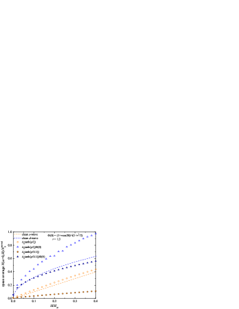
Figure 3: (Color online) The spatially averaged ZDOS, normalized to the normal state value $N(\omega=0)/N_{0}$ for a nodeless (orange) and a nodal (blue) single-band superconductor. The dashed lines show the idealized linear $H$ and $\sqrt{H}$ behavior for a clean $s$-wave and $d$-wave SC, respectively. The symbols are numerical results for a single band SC with an isotropic $s$-wave gap (circles) and a strongly anisotropic nodal gap (triangles). Additionally we compare results with (solid symbols) and without (open symbols) taking into account the vortex core reduction due to the Kramer-Pesch effect. Here we have ignored the field dependence of the superconducting gap, i.e. $\Delta(H)=\Delta_{0}$.

The superconducting order parameters in the two bands are related by the interband component of the pairing interaction. We consider a general coupling matrix in the factorized form, $\lambda_{\nu\mu}(\theta,\theta^{\prime})=\lambda_{\nu\mu}\Phi_{\nu}(\theta)\Phi_{\mu}(\theta^{\prime})$, where $\mu,\nu=1,2$ and $\lambda_{\nu\mu}\equiv V_{\nu\mu}N_{\mu}$. Here $V_{11}=V_{e}$ and $V_{22}=V_{h}$ are the intraband pairing interactions in the electron and the hole band, respectively, while $V_{12}=V_{eh}$ is the interband interaction. $N_{\mu}$ is the normal density of states at the Fermi level. Then the gap equation for an inhomogeneous superconductor is

$$\Delta_{\nu}(\mathbf{r})=2\pi T\sum_{\mu=1,2}\lambda_{\nu\mu}\sum_{\omega_{n}>0}^{\omega_{c}}\langle\Phi_{\mu}(\theta)f_{\mu}(\mathbf{r},\theta,i\omega_{n})\rangle_{\theta}\,.$$ (10)

Here $\Delta_{\nu}(\mathbf{r})$ is the momentum independent part of the gap function; $\Delta_{1,2}=\Delta_{0}^{e,h}$ at $T=0$ and $H=0$.

In the vortex state the self consistent determination of the spatially dependent order parameter is a complex task. Since we are interested in relatively low fields, when the vortices are well separated, we solve the Eilenberger equations for the order parameter that is assumed to have a single vortex form,

$$\Delta^{e}(\vec{\rho},H;\theta) =\Delta_{1}(H)\tanh\left(\frac{\rho}{0.1\xi_{0}^{e}}\right)\frac{1+r\cos 2\theta}{\sqrt{1+r^{2}/2}},$$ (11a)

$$\Delta^{h}(\vec{\rho},H) =\Delta_{2}(H)\tanh\left(\frac{\rho}{0.1\xi_{0}^{h}}\right)\,.$$ (11b)

Here $\vec{\rho}=(\rho,\phi)$ is the two-dimensional projection of the radius vector in cylindrical coordinates, and factor of 0.1 is introduced to approximate the shrinking of the core size in the self-consistent treatment at low temperatures (Kramer-Pesch effect Kramer and Pesch (1974); Pesch and Kramer (1974)). This single vortex ansatz provides a qualitatively correct description of the low-field state, close to what is found by full numerical solution. Dahm et al. (2002) To account for the suppression of the bulk order parameter by the magnetic field, we determine the coefficients $\Delta_{1,2}(H)$ from the Pesch approximation, Pesch (1975) where in the presence of an Abrikosov lattice the diagonal components of the Green’s function by its value averaged over a unit cell of the vortex lattice. This approximation proven to give reliable results over a considerable range of magnetic fields and is incorporated into our approach.

Note that our ansatz for the order parameter becomes quantitatively inaccurate for strong interband coupling in the regime of applicability of the Ginzburg-Landau theory since the core sizes of the two bands approach each other. Zhitomirsky and Dao (2004) We verified in a fully self-consistent calculation that in the parameter range that we use the corresponding effect on the specific heat is of order 1% or less and hence can be neglected. We therefore use Eq. (11) hereafter.

To proceed we substitute Eq. (11) into Eq. (6), solve for $a(x)$ and $b(x)$, and use Eq. (8) to find the local density of states $N(\vec{\rho},H)$. To approximate the specific heat coefficient, we evaluate the spatial average of the zero energy local density of states

$$\bar{N}(H)=\int_{0}^{2\pi}d\phi\int_{0}^{R}d\rho\,\rho\frac{N(\vec{\rho},H)}{\pi R^{2}N_{0}},$$ (12)

where the intervortex distance $R$ depends on $H$ as described by Eq. (9). The total density of states is then given as

$$\bar{N}(H)_{\text{tot}} =\frac{w_{e}\bar{N}^{e}(H)+w_{h}\bar{N}^{h}(H)}{w_{e}+w_{h}}$$ (13)

where $w_{e}/w_{h}=2N_{0}^{e}/N_{0}^{h}=2\zeta$ if we consider, for example, two electron Fermi surface sheets in the folded Brillouin zone and denote $\zeta\equiv N_{0}^{e}/N_{0}^{h}=v_{F}^{h}/v_{F}^{e}=0.65=\lambda_{21}/\lambda_{12}$.

IV Results

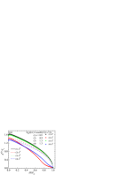
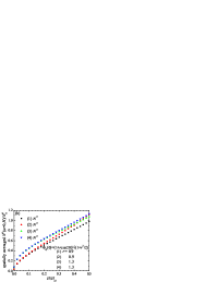
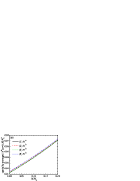
Figure 4: (Color online) Results of quasiclassical calculations for the parameters in Table I.(a) Magnetic field dependence of the gaps in the two-band model calculated within the Pesch approximation Pesch (1975); Klimesch and Pesch (1978) for case (1) - (4). We assume $\Delta^{e}(H=0)=\Delta^{h}(H=0)$ here. The four sets of coupling constants $\lambda_{ij}$ are listed in TABLE 1. (b) Field dependence of the space average ZDOS $N^{e}(H)$ on the electron pocket for the four cases with anisotropic gap with angular variation $\Phi_{e}(\theta)=(1+r\cos 2\theta)/\sqrt{1+r^{2}/2}$. (c) Field dependence of the space average ZDOS $N^{h}(H)$ for the four cases with isotropic gap along the hole pocket.

To illustrate that the salient features of the vortex state DOS are captured in our approach in Fig. 3 we show the field dependence of the spatially averaged zero energy local density of states (ZDOS) for a one-band SC with either an isotropic $s$-wave gap or a strongly anisotropic nodal gap ($r=1.3$). Note that, while the field dependences in both the nodal and fully gapped cases clearly fit the anticipated power laws at low fields, $\sqrt{H}$ and $H$, respectively, there is a significant influence on the magnitude of the DOS caused by the size of the core, with the smaller core size yielding smaller ZDOS. In particular, in the absence of the Kramer-Pesch effect, for the nodal case the ZDOS would exceed the normal state value at fields far below $H_{c2}$, which is unphysical.

Below we consider $r=0.9$ and $r=1.3$ to mimic a gap with deep minima and accidental nodes, respectively. To show different types of behavior allowed within our microscopic model we chose four sets of coupling constants, two for each value of $r$, as shown in Table 1. In cases (1) and (3), the interband pairing $\lambda_{12}$ is strong and close to the intraband parameter $\lambda_{11}$, while in case (2) and (4) $\lambda_{12}\ll\lambda_{11},\lambda_{22}$.

Table 1: The different models for the coupling matrix and the gap anisotropy on the electron pockets considered in this work.

	$\lambda_{11}$	$\lambda_{12}$	$\lambda_{21}$	$\lambda_{22}$	$r$	$T_{c}/$K	$H_{c2}/$T
case (1)	0.51	0.51	0.33	0.65	0.9	31	54
case (2)	1.00	0.02	0.013	0.81	0.9	31	47
case (3)	0.51	0.51	0.34	0.64	1.3	31	54
case (4)	1.00	0.023	0.015	0.77	1.3	31	42

In Fig. 4(a) we show the self-consistently determined magnitudes of the bulk gaps in the vortex state $\Delta_{1,2}(H)$ as defined in Eq. (10) and (11). $H_{c2}\sim 40-50$ T. In the cases with only weak interband pairing (2) and (4), the gap on the electron Fermi surface deviates considerably from the phenomenological form $\Delta(H)=\Delta_{0}\sqrt{1-H/H_{c2}}$. Figs. 4(b) and (c) show the spatially averaged ZDOS corresponding to each band. For $N^{e}(H)$ and for $r=1.3$ the $\sqrt{H}$ behavior of the Volovik effect is clearly visible at lower fields. Comparing Fig. 4(b) to Fig. 3 we find that within the two-band model the density of states on the electron band $N^{e}(H)$ reaches a quasi-linear behavior already at smaller fields than the corresponding density of states for the one-band case. In Fig. 3 a linear behavior is never observed, and might only be fit over some intermediate field range for $H/H_{c2}>0.2$, while in the multiband case $N^{e}(H)$ displays a clear linear behavior already for $H/H_{c2}>0.1$.

It is tempting to interpret the low-field crossover to a quasilinear field variation as evidence for a small energy scale $\Delta_{sm}\equiv\Delta_{0}^{e}(1-r)/\sqrt{1+r^{2}/2}$ on the electron band; this, however, seems unlikely. Provided $\Delta_{sm}\ll\Delta_{0}^{e}$, the gap still increases linearly along the Fermi surface away from the nodal points above this energy scale, simply with a different slope. Then within the usual Volovik argumentation the contributions from extended states at these intermediate energies give rise to a $\sqrt{H}$ contribution even if $\Delta_{sm}\lesssim E_{H}\ll\Delta_{max}$, where $E_{H}\propto\sqrt{H}$ is the average Doppler shift and $\Delta_{max}\equiv\Delta_{0}^{e}(1+r)/\sqrt{1+r^{2}/2}$ is the maximum gap. There is therefore no true linear-$H$ behavior arising from the electron band with gap nodes. Consequently, we interpret this crossover as the consequence of the two-band behavior coupled with a gradually increasing contribution of core states which is nearly linear in field. Fig. 4(c) clearly shows that the density of states on the hole band $N^{h}(H)$, assumed here to be fully gapped, is always linear as a function of field and the results for the two different coupling matrices considered here are very similar. However, as mentioned before, the slope is smaller than the one predicted for an idealized $s$-wave SC.

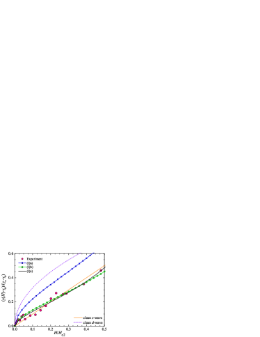
Figure 5: (Color online) Comparison of the experimentally measured normalized specific heat coefficient (large pink dots) to different theoretical results for the spatially averaged ZDOS. The dotted violet and solid orange curves are the predictions for the spatially averaged ZDOS for a clean $s$-wave and $d$-wave SC. The blue squares (case (Qa)) and green diamonds (case (Qb)) are the differently weighted sums of $\bar{N}^{e}(H)$ and $\bar{N}^{h}(H)$ evaluated for case (4) of Figs. 4(b) and (c). The black line (case (Qc)) is obtained using the formula $\gamma^{\text{tot}}=a_{1}\bar{N}_{e}(H)+a_{2}\bar{N}_{h}(H)$ where $a_{1}=3.2$ mJ/(mole K²), $a_{2}=10.3$ mJ/(mole K²) are determined with the least square fit to experimental data below 30 T. Note “$d$-wave” and “$s$-wave” curves represent simple extrapolations of the low-field $\sqrt{H}$ and $H$ terms up to $H_{c2}$.

Using Eq. (13), the spatially averaged ZDOS on the electron and the hole band are added with different weights. Using the results presented in Figs. 4(b) and (c) as case (4), we investigate several cases. Since there are two electron pockets, and assuming that only one hole pocket contributes significantly to the low energy density of states (or that a naive average over the hole pockets is sufficient), the net DOS and the field dependence of the Sommerfeld coefficient are only functions of the ratio of the densities of states on the electron and hole sheets. In the following we will study three cases that we will abbreviate with “Q” indicating the use of the quasiclassical, or Eilenberger, approach:

• (Qa): we assume that only one hole pocket contributes considerably to the low energy DOS, and use the weights $w_{e}/w_{h}=2N_{0}^{e}/N_{0}^{h}$ taken from the DFT calculation, $N_{0}^{e}/N_{0}^{h}=0.65$, see Ref. Mishra et al., 2011;

• (Qb): We once again fix $N_{0}^{e}/N_{0}^{h}=0.65$, but adopt a model for which the normal DOS for all three hole pockets of Ba₂Fe₂(As_0.7P_0.3)₂ are the same and for which all three pockets contribute equally to the low energy DOS, hence $w_{e}/w_{h}=2N_{0}^{e}/3N_{0}^{h}$;

• (Qc): We do not hold the ratio $N_{0}^{e}/N_{0}^{h}$ fixed, but instead calculate the weights for the electron pockets $a_{1}$ and for the hole pockets $a_{2}$ by a least squares fit to the experimental data using the formula $\gamma^{\text{tot}}=a_{1}\bar{N}_{e}(H)+a_{2}\bar{N}_{h}(H)$. If we normalize it to the presumed contribution of the superconducting fraction, $\gamma_{n}-\gamma_{0}\approx 14$ mJ/(mole K²), where $\gamma_{0}$ is the extraneous term, see below, we find $w_{e}/(w_{e}+w_{h})=a_{1}/(\gamma_{n}-\gamma_{0})$ and $w_{h}/(w_{e}+w_{h})=a_{2}/(\gamma_{n}-\gamma_{0})$ and $a_{1}/a_{2}=w_{e}/w_{h}$.

In Fig. 5 we compare the results for all three cases to the experimentally measured specific heat coefficient (pink dots). The experimental values are obtained by extrapolating the measured specific heat coefficient $\gamma$ at various temperatures to $T=0$. The upper critical field $H_{c2}$ is taken to be 52 T, see Ref. Yamashita et al., 2011. The normal state $\gamma_{n}=16$ mJ/(mol K²) can be obtained by extrapolating $\gamma$ to $H_{c2}$. A substantial residualKim et al. (2010) $\gamma_{0}=1.7$ mJ/(mol K²) in the superconducting state, presumed due to disorder, is subtracted in the plots of the field dependence from the experimental data (pink dots) to compare with our quasiclassical calculation in the clean limit (blue squares and green diamonds). Note that subtracting of the residual C/T tends to enhance the scatter in the low-T data of Fig 2.

From Fig. 5, we see that the results derived for model (Qb) with three equal mass hole pockets and two equal mass electron pockets are in good agreement with the experimental data: both experiment and theory show a “Volovik effect” at the lowest fields and then a crossover to a linear $H$ dependence at intermediate fields. While model (Qa) has the same qualitative behavior, the relative weights of hole and electron bands are apparently not consistent with the normalized experimental data, and the fit is much poorer. Compared to (Qb) the least squares fit (Qc) to the experimental data (black line) is only marginally improved, and gives $N_{0}^{e}/N_{0}^{h}=0.47$ with two electron pockets/three hole pockets or $0.16$ with two electron pockets/one hole pocket, same order as obtained from DFT.

For completeness it is important to determine whether the experimental data can be appropriately fit within the confines of a simple two-band Doppler shift approach. We detail this method in the Appendix, where we show that models (a) and (b) do not give a satisfactory fit to the experiment. In contrast, model (c) yields a rather similar field dependence of the field-induced enhancement of the Sommerfeld coefficient for the quasiclassical and Doppler (Dc) methods, as shown in Fig. 6. At the same time the best fit linear coefficients for (Dc), $a_{1}=1.50$ mJ/(mole K²), $a_{2}=65.6$ mJ/(mole K²), give the ratio of the normal state DOS for two electron/three hole Fermi sheets of $N_{0}^{e}/N_{0}^{h}=3a_{1}/2a_{2}\approx 0.03$, very different from the value of 0.65 obtained within the band structure calculations. Consequently, the quasiclassical methods provides a far more satisfying fit to the data.

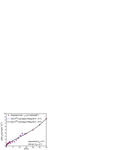
Figure 6: (Color online) $\gamma^{\text{tot}}$ plotted with experimental data in absolute units. Case (Qc) is the similar black line in Fig. 5. (Dc) is obtained using formula $\gamma^{\text{tot}}=a_{1}\bar{N}_{e}(H)+a_{2}\bar{N}_{h}(H)$, where $\bar{N}_{e}(H)$ and $\bar{N}_{h}(H)$ are represented by the open squares and circles in Fig. 8 and $a_{1}=1.50$ mJ/(mole K²), $a_{2}=65.6$ mJ/(mole K²) for (Dc) are determined with the least square fit to the experimental data below 15 T.

As is usually the case with the measurements that probe the amplitude rather than the phase of the gap, it is difficult to distinguish the deep minima from the nodes. In this case we find that with our current uncertainty in the band parameters, and the scatter in the data, it is impossible to assert the nodal behavior purely from the current data. Fig. 7 shows the comparison of cases (1) and case (4) of Table 1, corresponding to $r=1.3$ and 0.9, i.e. with and without true nodes, with the weights of case (Qb). Even though the nodal fit appears better at the lowest fields, higher $H$ data are in between the two cases. Therefore the conclusion about the true node comes from the data on other experiments, such as penetration depth.

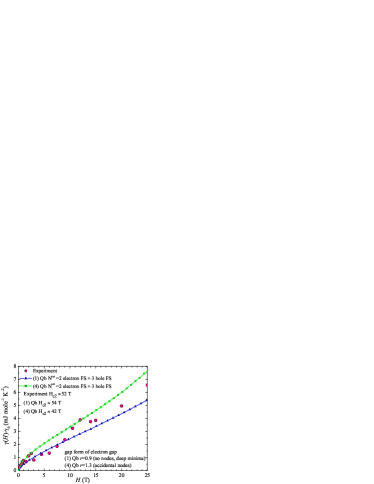
Figure 7: (Color online) Experimentally measured specific heat coefficient (large pink dots) compared to calculations with deep gap minima (case (1), $r=0.9$, blue triangles) and accidental nodes (case (4), $r=1.3$, green squares). In both cases the weight of electron and hole pocket contributions has been chosen in agreement with case (Qb).

V Conclusions

Among the various families of Fe-based superconductors, BaFe₂(As_1-xP_x)₂ may be a key system for understanding the origins of superconductivity. In part this is because, alone among the materials thought to display nodes in the superconducting gap, it possesses a rather high $T_{c}$ of 31 K, and hence the interplay of the pairing mechanism and Fermi surface shape and parameters in determining the gap anisotropy is under special scrutiny. The lack of an observable Volovik effect in earlier specific heat measurements was a cautionary note in an otherwise consistent array of measurements in support of gap nodes. In this paper, we have presented new experimental data at both lower and higher fields than previous measurements, and found that the initially reported linear-$H$ behavior extends up to 35 T, but that at low fields ($H\lesssim 4$ T) more precise measurements with smaller gradations in the change of field between data points are now clearly consistent with a Volovik-type effect. The residual $T\to 0$ Sommerfeld coefficient $\gamma(T\to 0)$ is about 1.7 mJ/mol-K², consistent with possible nanoscale disorder in the sample. The low-field sublinear dependence of the Sommerfeld coefficient is a strong indication that nodes (or deep minima) are present, and provides the sought-after consistency with other probes without having to make extreme assumptions about the ratio of masses on electron pockets to those on hole pockets, as was proposed in Ref. Kim et al., 2010.

It is nevertheless striking that indications of nodal behavior on the same samples is so much weaker in the specific heat measurements as compared to thermal conductivity and penetration depth. This is clearly indicating that the nodes are located on the pockets with smaller masses and/or longer lifetimes, as was pointed out in Ref. Kim et al., 2010. We have attempted to put this statement on a semiquantitative basis by presenting a quasiclassical (Eilenberger) calculation of the density of states and specific heat of a two-band anisotropic $s_{\pm}$ superconductor. Comparison with the Doppler shift method allowed us to argue that the quasiclassical calculation is superior for semiquantitative purposes. We find that the unusually small range of Volovik-type behavior, followed by a large range of linear-$H$ behavior, is due to the small gap and weak nodes on the small mass (presumably electron) sheet.Kim et al. (2010); Yamashita et al. (2011) Good fits to the data are obtained for average hole and electron maximum gaps of approximately equal magnitude, in the weak interband coupling limit. The success of this fit should not, however, tempt one to draw definitive conclusions about the relative magnitudes of the pairing interactions. The proliferation of parameters in the theory make it difficult to determine gap magnitudes, density of states ratios, and nodal properties with any quantitative certainty. Equally good fits can be obtained, for example, with substantially smaller full gaps than anisotropic gaps; the nodes control the low-field behavior, and the small full gap gives rise to a large linear term. What is important is that we have shown that a fit can be obtained, with reasonable values of the parameters, that it can only be obtained if nodes exist on one of the Fermi sheets, and that it requires going beyond the simple Doppler shift picture. It is our hope that the results of this calculation and fit will eventually lead to a more quantitative first principles based calculation.

Appendix A Comparison with the Doppler-shift method

In the following we briefly discuss the basic concepts of the Doppler-shift method and compare it to the quasiclassical approximation as manifested in the formulation of the Eilenberger equations introduced in the main text. The Doppler shifted energy due to the local supercurrent flow is $\omega-m\mathbf{v}_{F}\cdot\mathbf{v}_{s}(\mathbf{r})$ where

$$m\mathbf{v}_{F}^{e,h}\cdot\mathbf{v}_{s}(\mathbf{r}) =\frac{\hbar}{2|\mathbf{r}|}\mathbf{v}_{F}^{e,h}(\theta)\cdot\mathbf{e}_{\phi}=\frac{\hbar v_{F}^{e,h}}{2|\mathbf{r}|}\sin(\theta-\phi)$$

$$=\frac{\Delta_{0}^{e,h}}{2\tilde{\rho}^{e,h}}\sin(\theta-\phi).$$ (14)

Here, we assume $\Delta^{e}(T=0,H=0)=\Delta^{h}(T=0,H=0)=\Delta_{0}^{e,h}$ and use $\tilde{\rho}^{e,h}=|\mathbf{r}|/\xi_{0}^{e,h}$. Therefore the normalized local DOS is

$$N(\omega,\mathbf{r})=\int_{0}^{2\pi}\frac{d\theta}{2\pi}$$

$$\mathrm{Re}\,\left\{\frac{|\omega-m\mathbf{v}_{F}\cdot\mathbf{v}_{s}(\mathbf{r})|}{\sqrt{(\omega-m\mathbf{v}_{F}\cdot\mathbf{v}_{s}(\mathbf{r}))^{2}-|\Delta(\theta)|^{2}}}\right\},$$ (15)

and thus the normalized spatially averaged DOS is

$$\bar{N}(H)=\int_{0}^{\tilde{R}}\frac{d\tilde{\rho}\;\tilde{\rho}}{\pi\tilde{R}^{2}}\int_{0}^{2\pi}d\phi\int_{0}^{2\pi}\frac{d\theta}{2\pi}$$

$$\mathrm{Re}\left\{\frac{|\omega-\Delta_{0}\sin(\theta-\phi)/(2\tilde{\rho})|}{\sqrt{\left[\omega-\Delta_{0}\sin(\theta-\phi)/(2\tilde{\rho})\right]^{2}-|\Delta(\theta)|^{2}}}\right\}.$$ (16)

Here we have introduced the normalized vortex cell radius $\tilde{R}=R/\xi_{0}^{e}$ for the electron bands or $R/\xi_{0}^{h}$ for the hole bands, respectively. Since the Doppler-shift method does not capture core state contributions it underestimates the slope of the magnetic field dependence of the zero energy DOS of an $s$-wave SC. Since the core region only gives negligible contributions to the total DOS one can in principle avoid the divergence of the Doppler-shift energy as $\tilde{\rho}\rightarrow 0$ by cutting out the complete core region with a lower limit $\xi_{0}$ for the radial integration. Here we have included the core region when integrating over the vortex unit cell. To model $\Delta(\theta)$ we use a similar function as given by Eq. (11), but without explicitely modeling the core structure

$$\Delta^{e}(\vec{\rho};\theta) =\Delta_{1}(H=0)\frac{1+r\cos 2\theta}{\sqrt{1+r^{2}/2}},$$ (17a)

$$\Delta^{h}(\vec{\rho}) =\Delta_{2}(H=0),$$ (17b)

and we use the self-consistently calculated $\Delta_{1,2}(H=0)$ in case (4) of the quasiclassical calculation in which the anisotropy factor $r=1.3$ for the gap along the electron Fermi surface sheet and the ratio of the normal DOS at the Fermi energy is taken as $N_{0}^{e}/N_{0}^{h}=0.65$.

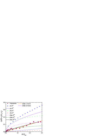
Figure 8: (Color online) Normalized specific heat coefficient determined within the quasiclassical approach (blue triangles and blue dashed curve) and within the Doppler-shift method (open squares and circles). Total normalized specific heat coefficients obtained within Doppler-shift method are shown by magenta dots, olive dash-dots and black solid line for cases (Da, Db, Dc), corresponding to (Qa, Qb, Qc), respectively. The dotted violet and solid orange curves are the power laws predicted for the spatially averaged ZDOS of an idealized $s$-wave and $d$-wave SC. Large pink dots show the experimentally determined normalized specific heat coefficient.

In Fig. 8 we show the results obtained within the Doppler-shift approach and compare them to case (4) of the quasiclassical method. Again we also show predictions for an idealized clean $s$- and $d$-wave SC. We conclude that the Doppler-shift method and the quasiclassical method give comparable results at lowest fields but start to deviate as soon as the field increases. One reason might be that with increasing field and decreasing inter-vortex distance the core states that are not correctly accounted for within the Doppler-shift method but captured within the quasiclassical approach become increasingly more important. However, due to the limitations of the single vortex approximation the overlapping of vortices is not correctly reproduced and the DOS is overestimated (In Fig. 8 the blue triangles rise too fast).

In Fig. 6 we compare the least squares fit by Doppler-shift method (blue dashed curve) together with least square fit by quasiclassical method (the similar black line from Fig. 5) and experimental data (large pink dots). The linear coefficients for (Dc) are $a_{1}=1.50$ mJ/(mole K²), $a_{2}=65.6$ mJ/(mole K²). Compared to the linear coefficients for (Qc) ($a_{1}=3.2$ mJ/(mole K²), $a_{2}=10.3$ mJ/(mole K²)), they give a nonphysical ratio of the normal DOS at Fermi energy if we consider two electron Fermi sheets and three hole Fermi sheets. To see this point, let’s consider equation

$$C_{e,h}(T,H) =\frac{1}{2}\int_{-\infty}^{+\infty}d\omega\frac{\omega^{2}\tilde{N}_{e,h}(H,\omega)}{T^{2}\cosh(\omega/2T)}$$ (18)

$$\approx A\tilde{N}_{e,h}(H,\omega)T\quad\quad(\text{as $T\to 0$})$$

$$\Rightarrow\gamma_{e,h} \approx A\tilde{N}_{e,h}(H,0)\equiv AN_{0}^{e,h}\bar{N}_{e,h}(H,0).$$

Here $A$ is a numeric constant and we write $\tilde{N}_{e,h}(H,0)\equiv N_{0}^{e,h}\bar{N}_{e,h}(H,0)$ where $\bar{N}_{e,h}(H,0)$ is the ZDOS calculated by the Green’s function method as defined in Eq. (12). Denote the number of Fermi sheets included in summation as $n_{FS}$ and define $n_{FS}^{e}AN_{0}^{e}=a_{1}$ and $n_{FS}^{h}AN_{0}^{h}=a_{2}$ (equivalent to $w_{e}=n_{FS}^{e}N_{0}^{e}$ and $w_{h}=n_{FS}^{h}N_{0}^{h}$). Therefore $\gamma^{\text{tot}}=a_{1}\bar{N}_{e}(H)+a_{2}\bar{N}_{h}(H)$. Note $\bar{N}_{e,h}(H)$ are dimensionless and $a_{1,2}$ are in unit of $\mathrm{mJ/(mole\,K^{2})}$. Optimized parameters $a_{1,2}$ for least square fit (Dc) to the experimental data below 15 T are $a_{1}=1.50$ and $a_{2}=65.6$. This leads to our estimate in the main text of $a_{1}/a_{2}=(n_{FS}^{e}AN_{0}^{e})/(n_{FS}^{h}AN_{0}^{h})=(2N_{0}^{e})/(3N_{0}^{h})$, and $N_{0}^{e}/N_{0}^{h}=0.03$, and to our conclusion that Doppler-shift method does not provide a satisfying physical explanation to our specific heat experiment.

References

- Kamihara et al. (2008) Y. Kamihara, T. Watanabe, M. Hirano, and H. Hosono, Journal of the American Chemical Society 130, 3296 (2008).
- Hsu et al. (2008) F. Hsu, J. Luo, K. Yeh, T. Chen, T. Huang, P. Wu, Y. Lee, Y. Huang, Y. Chu, D. Yan, et al., Proceedings of the National Academy of Sciences 105, 14262 (2008).
- Wen (2011) H. Wen, Annual Review of Condensed Matter Physics 2, 121 (2011).
- Stewart (2011) G. Stewart, arXiv:1106.1618 (2011).
- Kemper et al. (2010) A. Kemper, T. Maier, S. Graser, H. Cheng, P. Hirschfeld, and D. Scalapino, New Journal of Physics 12, 073030 (2010).
- Hirschfeld et al. (2011) P. Hirschfeld, M. Korshunov, and I. Mazin, arXiv:1106.3712 (2011).
- Kasahara et al. (2010) S. Kasahara, T. Shibauchi, K. Hashimoto, K. Ikada, S. Tonegawa, R. Okazaki, H. Shishido, H. Ikeda, H. Takeya, K. Hirata, T. Terashima, and Y. Matsuda, Phys. Rev. B 81, 184519 (2010).
- Jiang et al. (2009) S. Jiang, H. Xing, G. Xuan, C. Wang, Z. Ren, C. Feng, J. Dai, Z. Xu, and G. Cao, Journal of Physics: Condensed Matter 21, 382203 (2009).
- Shishido et al. (2010) H. Shishido, A. F. Bangura, A. I. Coldea, S. Tonegawa, K. Hashimoto, S. Kasahara, P. M. C. Rourke, H. Ikeda, T. Terashima, R. Settai, Y. Ōnuki, D. Vignolles, C. Proust, B. Vignolle, A. McCollam, Y. Matsuda, T. Shibauchi, and A. Carrington, Phys. Rev. Lett. 104, 057008 (2010).
- Hashimoto et al. (2010) K. Hashimoto, M. Yamashita, S. Kasahara, Y. Senshu, N. Nakata, S. Tonegawa, K. Ikada, A. Serafin, A. Carrington, T. Terashima, H. Ikeda, T. Shibauchi, and Y. Matsuda, Phys. Rev. B 81, 220501 (2010).
- Nakai et al. (2010) Y. Nakai, T. Iye, S. Kitagawa, K. Ishida, S. Kasahara, T. Shibauchi, Y. Matsuda, and T. Terashima, Phys. Rev. B 81, 020503 (2010).
- Yamashita et al. (2011) M. Yamashita, Y. Senshu, T. Shibauchi, S. Kasahara, K. Hashimoto, D. Watanabe, H. Ikeda, T. Terashima, I. Vekhter, A. B. Vorontsov, and Y. Matsuda, Phys. Rev. B 84, 060507 (2011).
- Kim et al. (2010) J. S. Kim, P. J. Hirschfeld, G. R. Stewart, S. Kasahara, T. Shibauchi, T. Terashima, and Y. Matsuda, Phys. Rev. B 81, 214507 (2010).
- Note (1) In contrast to BaFe2(As1-xPx)2, recent high field measurements on underdoped () and overdoped () BaFe2-xCoxAs2 have found that the specific heat coefficient varies approximately as all the way up to . J. S. Kim, G. R. Stewart, K. Gofryk, F. Ronning, and A. S. Sefat, to be published.
- Bang (2010) Y. Bang, Phys. Rev. Lett. 104, 217001 (2010).
- Kogan and Schmalian (2011) V. G. Kogan and J. Schmalian, Phys. Rev. B 83, 054515 (2011).
- Stewart (1983) G. Stewart, Review of Scientific Instruments 54, 1 (1983).
- Andraka et al. (1989) B. Andraka, G. Fraunberger, J. S. Kim, C. Quitmann, and G. R. Stewart, Phys. Rev. B 39, 6420 (1989).
- Kim et al. (2009) J. Kim, E. Kim, and G. Stewart, Journal of Physics: Condensed Matter 21, 252201 (2009).
- Eilenberger (1968) G. Eilenberger, Z. Phys. 214, 195 (1968).
- Larkin and Ovchinnikov (1969) A. I. Larkin and Y. N. Ovchinnikov, Sov. Phys. JETP 28, 1200 (1969).
- Serene and Rainer (1983) J. Serene and D. Rainer, Physics Reports 101, 221 (1983).
- Volovik (1993) G. E. Volovik, JETP Lett. 58, 469 (1993).
- Moler et al. (1997) K. A. Moler, D. L. Sisson, J. S. Urbach, M. R. Beasley, A. Kapitulnik, D. J. Baar, R. Liang, and W. N. Hardy, Phys. Rev. B 55, 3954 (1997).
- Wang et al. (2001) Y. Wang, B. Revaz, A. Erb, and A. Junod, Phys. Rev. B 63, 094508 (2001).
- Ichioka et al. (1996) M. Ichioka, N. Hayashi, N. Enomoto, and K. Machida, Phys. Rev. B 53, 15316 (1996).
- Schopohl and Maki (1995) N. Schopohl and K. Maki, Phys. Rev. B 52, 490 (1995).
- Ichioka et al. (1997) M. Ichioka, N. Hayashi, and K. Machida, Phys. Rev. B 55, 6565 (1997).
- Ichioka et al. (1999) M. Ichioka, A. Hasegawa, and K. Machida, Phys. Rev. B 59, 184 (1999).
- Franz and Tevsanović (2000) M. Franz and Z. Tevsanović, Phys. Rev. Lett. 84, 554 (2000).
- Vekhter and Vorontsov (2008) I. Vekhter and A. Vorontsov, Physica B: Condensed Matter 403, 958 (2008).
- Dahm et al. (2002) T. Dahm, S. Graser, C. Iniotakis, and N. Schopohl, Phys. Rev. B 66, 144515 (2002).
- Schopohl (1998) N. Schopohl, cond-mat/9804064 (unpublished) (1998).
- Note (2) Note that our notation of , , and differs from the one used in Ref. \rev@citealpnumschopohl98. Under the transformation , , and the notation in Ref. \rev@citealpnumschopohl98 passes into our notation.
- Suzuki et al. (2011) K. Suzuki, H. Usui, and K. Kuroki, Journal of the Physical Society of Japan 80, 013710 (2011).
- Shimojima et al. (2011) T. Shimojima, F. Sakaguchi, K. Ishizaka, Y. Ishida, T. Kiss, M. Okawa, T. Togashi, C. Chen, S. Watanabe, M. Arita, et al., Science 332, 564 (2011).
- Mishra et al. (2009) V. Mishra, G. Boyd, S. Graser, T. Maier, P. J. Hirschfeld, and D. J. Scalapino, Phys. Rev. B 79, 094512 (2009).
- Mishra et al. (2011) V. Mishra, S. Graser, and P. J. Hirschfeld, ArXiv e-prints (2011), arXiv:1101.5699 [cond-mat.supr-con] .
- Yoshida et al. (2011) T. Yoshida, I. Nishi, S. Ideta, A. Fujimori, M. Kubota, K. Ono, S. Kasahara, T. Shibauchi, T. Terashima, Y. Matsuda, H. Ikeda, and R. Arita, Phys. Rev. Lett. 106, 117001 (2011).
- Kramer and Pesch (1974) L. Kramer and W. Pesch, Z. Phys. 269, 59 (1974).
- Pesch and Kramer (1974) W. Pesch and L. Kramer, J. Low T. Phys. 15, 367 (1974).
- Pesch (1975) W. Pesch, Z. Phys. B 21, 263 (1975).
- Zhitomirsky and Dao (2004) M. E. Zhitomirsky and V.-H. Dao, Phys. Rev. B 69, 054508 (2004).
- Klimesch and Pesch (1978) P. Klimesch and W. Pesch, J. Low T. Phys. 32, 869 (1978).