Thermal properties of a solid through $q$-deformed algebra

Abstract

We study the thermodynamics of a crystalline solid by applying $q$-deformed algebras. We based part of our study on both Einstein and Debye models, exploring primarily $q$-deformed thermal and electric conductivities as a function of Debye specific heat. The results revealed that $q$-deformation acts as a factor of disorder or impurity, modifying the characteristics of a crystalline structure, as for example, in the case of semiconductors.

I Introduction

Quantum groups and quantum algebras can be considered $q$-deformations of Lie groups and semi-simple Lie algebras anat . Physical systems with $q$-deformation have been the subject of intense research due to the emergence of quantum group structures caused by certain physical problems. This establishes a connection with $q$-analysis, known in mathematics for over a century. From the mathematical point of view, $q$-deformed algebra usually requires Hopf algebra. The $q$-deformation of a physical system is not the only way to deform it; rather, there are several ways of applying deformation in different physical and mathematical contexts sin ; tsallis .

For example, the widely studied harmonic oscillator system has several $q$-deformed descriptions bie ; mac . These are obtained from each other by transformation, as shown in borz ; flo . Some of the main problems in obtaining the $q$-oscillator are the spectrum, Hamiltonian, position and time operator. Moreover, the $q$-deformation of physical systems beyond the oscillator is not well studied. Most concepts of classical mechanics and quantum mechanics become unclear after being $q$-deformed day .

This study extends our previous analysis bri to solids. A solid consists of a large number of atoms linked by cohesive forces of various kinds. On the other hand, in a gas, molecules are free to move around the container, while in a liquid, they have less freedom, but still travel considerable distances. Atomic motion in a solid is very slight, causing every atom to move only within a small neighborhood, and vibrate around its equilibrium point. In a crystalline solid, the equilibrium points of atomic vibrations form a regular spatial structure, such as a cubic structure.

Interaction between atoms allows the propagation of elastic waves in solid media, which can be both horizontal and longitudinal. If atomic oscillations around equilibrium positions are small, which should occur at low temperatures, the potential interaction energy can be approximated by a quadratic form of atomic displacements. A crystalline solid, whose atoms interact according to this potential, is called a harmonic solid. In harmonic solids, elastic waves are harmonics and the normal modes of vibration in crystalline solids kit . A large number of phenomena involve quantum mechanical motion, in particular thermally-activated particles, obeying the $T^{3}$ law. Thermal excitations in the system are responsible for phonon excitation patt .

The study conducted by Anderson, Lee and Elliot and ; lee ; ell shows that the presence of defects or impurities in a crystal changes the electrostatic potential in their neighborhoods, breaking the translational symmetry of the periodic potential. This disturbance can produce electronic wave functions located near the impurity, ceasing to be propagated throughout the crystal.

The conductivity of semiconductors can also be dramatically altered by the presence of impurities, i.e., different from atoms that make up the pure crystal. This property enables the manufacture of a variety of electronic devices from the same semiconductor material. The process of placing impurities of known elements in a semiconductor is called doping. Next we see the application of $q$-deformation in solids acting as a defect or impurity, specifically in Einstein and Debye solids, and observe the consequences; for example, temperature and thermal conductivity in the Debye model and other features of chemical elements kit . We found interesting results, leading us to apply the same approach to other thermodynamic properties of solids, since this initial analysis shows that $q$-deformed elements have thermal properties are similar to another element in its pure state.

The paper is organized as follows: in Sec. II we present the $q$-deformed algebra; in Sec. III we implement $q$-deformation to Einstein and Debye solids in order to explore thermal properties; and finally, in Sec. IV we make our final comments.

II $q$-Deformed quantum algebra

The $q$-deformed algebra of the quantum oscillator is defined by $q$-deformed Heisenberg algebra in terms of creation and annihilation operators $a^{\dagger}$ and $a$, respectively, and quantum number $N$ by chai ; ng ; sak ,

$$[a,a]=[a^{\dagger},a^{\dagger}]=0\;,\qquad\qquad\ aa^{\dagger}-q^{-\frac{1}{2}}a^{\dagger}a=q^{\frac{N}{2}},$$ (1)

$$[N,a^{\dagger}]=a^{\dagger}\;,\qquad\qquad[N,a]=-a,$$ (2)

where deformation parameter $q$ is real and the observed value of $q$ has to satisfy the non-additivity property (see tsallis for a comprehensive study on this property in many physical issues)

$$[x+y]\neq[x]+[y].$$ (3)

In addition, the operators obey the relations

$$[N]=a^{\dagger}a\;,\quad\qquad\qquad aa^{\dagger}=[1+N].$$ (4)

The $q$-Fock space spanned by orthornormalized eigenstates ${|n\rangle}$ is constructed according to

$${|n\rangle}=\frac{(a^{\dagger})^{n}}{\sqrt{[n]!}}{|0\rangle},\qquad\qquad a{|0>}=0,$$ (5)

The actions of $a$, $a^{\dagger}$ and $N$ on the states ${|n\rangle}$ in the $q$-Fock space are known to be

$$a^{\dagger}{|n\rangle}=[n+1]^{1/2}{|n+1\rangle},$$ (6)

$$a{|n\rangle}=[n]^{1/2}{|n-1\rangle},$$ (7)

$$N{|n\rangle}=n{|n\rangle}.$$ (8)

The oscillator bie ; bie1 ; mac allows us to write the $q$-deformed Hamiltonian anat as follows:

$${\cal H}=\frac{1}{2}\Big{\{a,a^{\dagger}\Big{\}}}.$$ (9)

We have the basic $q$-deformed quantum number $n$ defined as erns ,

$$[x]=\frac{q^{\frac{x}{2}}-q^{-\frac{x}{2}}}{q^{\frac{1}{2}}-q^{-\frac{1}{2}}}\equiv[N]=a^{\dagger}a=\frac{q^{\frac{N}{2}}-q^{-\frac{N}{2}}}{q^{\frac{1}{2}}-q^{-\frac{1}{2}}}.$$ (10)

At limit $q\to 1$, the basic $q$-deformed quantum number $[x]$ is reduced to the number $x$. In our present study we shall not attempt to explicitly use Jackson derivative $(JD)$ jak ; jac to obtain $q$-deformed thermodynamics relations bri ; lav1 . Instead, we start with the $q$-deformed partition function and use ordinary derivatives to obtain $q$-deformed thermodynamics quantities.

III Implementation of the $q$-deformation

III.1 $q$-Deformed Einstein solid

We consider the solid in contact with a thermal reservoir at temperature $T$, where we have $n_{j}$ labeling the $j$-th oscillator. Given a microscopic state $\{n_{j}\}=\{n_{1},n_{2},\ldots,n_{N}\}$, the energy of this state can be written as

$$E\{n_{j}\}=\displaystyle\sum_{j=1}^{\infty}\left(n_{j}+\frac{1}{2}\right)\hbar\omega_{E},$$ (11)

Where $\omega_{E}$ is the Einstein frequency characteristic. As our primary purpose is $q$-deformation, we proceed to find the $q$-deformed version of (11). We can obtain $q$-deformed energies from the definition of the Hamiltonian (9), and the definitions provided earlier,

$$E_{n}=\frac{\hbar\omega_{E}}{2}\Big{(}[n]+[n+1]\Big{)}.$$ (12)

Considering the definition of basic number given in (10), and making $q=\exp(\gamma)$, we obtain flo

$$[n]=\frac{\sinh\left({\frac{n\gamma}{2}}\right)}{\sinh\left(\frac{\gamma}{2}\right)}.$$ (13)

Now replacing the equation (13) into equation (12), we have

$$E_{nq}=\frac{\hbar\omega_{E}}{2}\left[\frac{\sinh\left(\left(n+\frac{1}{2}\right)\frac{\gamma}{2}\right)}{\sinh\left(\frac{\gamma}{4}\right)}\right].$$ (14)

The partition function is given by

$$\Xi=\displaystyle\sum_{n_{j}}\exp(-\beta E\{n_{j}\}).$$ (15)

Since there is no interaction terms, we factored the sum and apply the result of equation (14) to obtain the $q$-deformed partition function

$$\Xi_{q}=\Bigg{\{}\displaystyle\sum_{n=0}^{\infty}\exp\left[-\beta E_{nq}\right]\Bigg{\}}^{N}=\Xi_{1_{q}}^{N},$$ (16)

where

$$\Xi_{1_{q}}=\frac{q^{\alpha_{q}}\exp\left(-2\alpha_{q}\left(\frac{\sqrt{q}-1}{\sqrt{q}+1}\right)\right)}{q^{\alpha_{q}}-1}.$$ (17)

As one knows $\beta=\frac{1}{\kappa_{B}T}$ and $\Theta_{E}$ is the Einstein temperature, defined by

$$\Theta_{E}=\frac{\hbar\omega_{E}}{\kappa_{B}},$$ (18)

and we define a $q$-deformed Einstein function $E(\alpha_{q})$ as

$$E(\alpha_{q})=q^{\alpha_{q}}\left(\frac{\alpha_{q}\gamma}{q^{\alpha_{q}}-1}\right)^{2},$$ (19)

$$\alpha_{q}=\frac{\Theta_{E}(\sqrt{q}+1)}{8T\sqrt[4]{q}\sinh\left(\frac{\gamma}{4}\right)}\equiv\frac{\Theta_{E}}{4T}\frac{\exp{(\frac{\gamma}{2})}+1}{\exp{(\frac{\gamma}{2})}-1}.$$ (20)

We can determine a $q$-deformed Helmholtz free energy per oscillator from the expression

$$\!\!\!\!\!\!\!\!f_{q} \!=\!-\frac{1}{\beta}\displaystyle\lim_{N\to\infty}\frac{1}{N}\ln\Xi$$ (21)

$$\!\!\!\!\!\!\!\!=\!\!\! \kappa_{B}T\Bigg{\{}2\alpha_{q}\!\left(\frac{\sqrt{q}-1}{\sqrt{q}+1}\right)-\ln(q^{\alpha_{q}})+\ln(q^{\alpha_{q}}-1\!)\!\Bigg{\}}.$$

By using the result of equation (21) we can determine the $q$-deformed entropy (see Fig. 1)

$$S_{q} =-\frac{\partial f}{\partial T}$$ (22)

$$= \kappa_{B}\Bigg{\{}\ln(q^{\alpha_{q}})-\ln(q^{\alpha_{q}}-1)+\frac{\alpha_{q}\ln(q)}{q^{\alpha_{q}}-1}\Bigg{\}}.$$

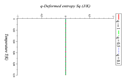
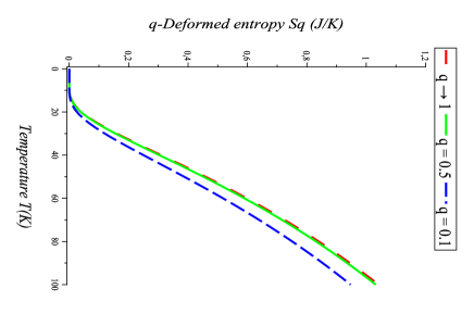
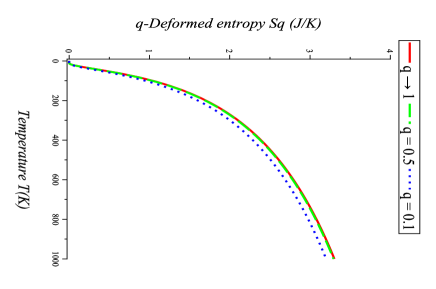
Figure 1: $q$-Deformed entropy $S_{q}$ vs temperature $T$ in the following intervals: $T=0$ to $T=0.1K$ (top), $T=0$ to $T=100K$ (center) and $T=0$ to $T=1000K$ (bottom).

The $q$-deformed specific heat can now be determined by

$$c_{Vq}(T) = T\left(\frac{\partial S_{q}}{\partial T}\right)$$ (23)

$$= \kappa_{B}q^{\alpha_{q}}\left(\frac{\ln(q)\alpha_{q}}{q^{\alpha_{q}}-1}\right)^{2}.$$

The specific heat of the Einstein solid as a function of $E(\alpha_{q})$, defined in equation (19), can be written as follows:

$$c_{Vq}(T)=3\kappa_{B}E(\alpha_{q}).$$ (24)

The complete behavior is depicted in Fig. 2. One should note that when $T\gg\theta_{E}$, with the ratio $\alpha=\frac{\theta_{E}}{T}\ll 1$, with $\theta_{E}$, for example, around $100K$ for common crystals, one recovers the classical result $c_{Vq}\to 3\kappa_{B}$, known as the Dulong-Petit law. However, for sufficiently low temperatures, where $T\ll\theta_{E}$ and therefore $\alpha\gg 1$, specific heat is exponential with temperature patt as

$$c_{Vq}\rightarrow\kappa_{B}\left(\frac{\theta_{E}}{T}\right)^{2}\exp\left(-\frac{\theta_{E}}{T}\right).$$ (25)

In general, the invariance of specific heat at high temperatures and its decrease at low temperatures show that the Einstein model is in agreement with experimental results. However, at sufficiently low temperatures, specific heat does not experimentally follow the exponential function given in equation (25). As for the $q$-deformed case we see a significant change in the curve when $q\to 0.1$ for intermediate temperatures. However, we will improve the model by following the Debye model and applying $q$-deformation in the next section.

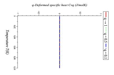
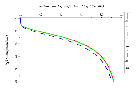
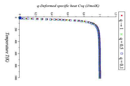
Figure 2: $q$-Deformed specific heat $c_{Vq}$ vs temperature $T$ in the following intervals: $T=0$ to $T=0.1K$ (top), $T=0$ to $T=100K$ (center) and $T=0$ to $T=1000K$ (bottom).

Finally, the $q$-deformed internal energy per oscillator as a function of temperature is given through

$$u_{q} = -\frac{\partial}{\partial\beta}\ln\Xi_{1_{q}}\qquad\qquad$$ (26)

$$= \kappa_{B}T\left[2\alpha_{q}\left(\frac{\sqrt{q}-1}{\sqrt{q}+1}\right)+\frac{\alpha_{q}\ln(q)}{(q^{\alpha_{q}}-1)}\right].$$

III.2 $q$-Deformed Debye solid

Corrections of Einstein’s model are given by the Debye model, allowing us to integrate from a continuous spectrum of frequencies up to the Debye frequency $\omega_{D}$, giving the total number of normal modes of vibration patt ; hua ; kit ; reif

$$\int_{0}^{\omega_{D}}g(\omega)d\omega=3N,$$ (27)

where $g(\omega)d\omega$ denotes the number of normal modes of vibration whose frequency is in the range $(\omega,\omega+d\omega)$. The function $g(\omega)$, can be given in terms of Rayleigh expression as following

$$8\pi\left(\frac{1}{\lambda}\right)^{2}d\left(\frac{1}{\lambda}\right)=\frac{\omega^{2}d\omega}{\pi^{2}c^{3}},$$ (28)

where $c$ is the speed of light and $\lambda$ wavelength. The expected energy value of the Planck oscillator with frequency $\omega_{s}$ is

$$<E_{s}>=\frac{\hbar\omega_{s}}{\exp\left(\frac{\hbar\omega_{s}}{\kappa_{B}T}\right)-1}.$$ (29)

Using equations (28) and (29), we obtain the energy density associated to the frequency range $(\omega,\omega+d\omega)$,

$$u(\omega)d\omega=\frac{\hbar}{\pi^{2}c^{3}}\frac{\omega^{3}d\omega}{\exp\left(\frac{\hbar\omega}{\kappa_{B}T}\right)-1}.$$ (30)

To obtain the number of photons between $\omega$ and $\omega+d\omega$, one makes use of the volume of the region on the phase space patt , which results in

$$g(\omega)d\omega\approx\frac{2V}{h^{3}}\left[4\pi\left(\frac{\hbar\omega}{c}\right)^{2}\left(\frac{\hbar d\omega}{c}\right)\right]=\frac{V\omega^{2}d\omega}{\pi^{2}c^{3}}.$$ (31)

Thus, replacing the equation (31) into equation (28), we can write the specific heat for any temperature. We now apply $q$-deformation in the same way as in equation (24),

$$c_{V_{q}}(T)=3\kappa_{B}D(\alpha_{0})_{q},$$ (32)

where $D(\alpha_{0})_{q}$ is the $q$-deformed Debye function, defined by

$$D(\alpha_{0})_{q}=\frac{3}{\alpha_{0_{q}}^{3}}\int_{0}^{\alpha_{0_{q}}}\frac{\alpha^{4}\exp{\alpha}}{[\exp(\alpha)-1]^{2}}d\alpha,$$ (33)

with

$$\alpha_{0_{q}}=\frac{\hbar\omega_{D_{q}}}{\kappa_{B}T}=\frac{\theta_{D_{q}}}{T},$$ (34)

and

$$\omega_{D_{q}}=\frac{\omega_{D}\sinh\left(\frac{\ln(q)}{2}\right)}{2\sinh\left(\frac{\ln(q)}{4}\right)},$$ (35)

where $\omega_{D_{q}}$ is the $q$-deformed Debye frequency and $\theta_{D_{q}}$ is the $q$-deformed Debye temperature. Integrating equation (33) by parts one finds

$$D(\alpha_{0})_{q}=-\frac{3\alpha_{0_{q}}}{\exp(\alpha_{0_{q}})-1}+\frac{12}{\alpha_{0_{q}}^{3}}\int_{0}^{\alpha_{0_{q}}}{\frac{\alpha^{3}d\alpha}{\exp(\alpha)-1}},$$ (36)

that can be integrated out to give the full expression

$$\!\!\!\!\!D(\alpha_{0})_{q}=$$ (37)

$$\!\!\!\!\!=\!\!\!\!\! 3\kappa_{B}\Biggl{\{}-\frac{3\alpha_{0_{q}}}{\exp{\left(\alpha_{0_{q}}\right)}-1}+\frac{12}{\alpha_{0_{q}}^{3}}\Bigg{[}-\frac{\pi^{4}}{15}-\frac{1}{4}\alpha_{0_{q}}^{4}+$$

$$\!\!\!\!\!+\!\!\!\!\! \alpha_{0_{q}}^{3}\ln\left[1-\exp\left(\alpha_{0_{q}}\right)\right]+3\left(\alpha_{0_{q}}\right)^{2}{\rm Li}_{2}\left[\exp\left(\alpha_{0_{q}}\right)\right]-$$

$$\!\!\!\!\!-\!\!\!\!\! 6\left(\alpha_{0_{q}}\right){\rm Li}_{3}\left[\exp\left(\alpha_{0_{q}}\right]\right)+6\ {\rm Li}_{4}\left[\exp\left(\alpha_{0_{q}}\right)\right]\Bigg{]}\Biggl{\}},$$

where

$${\rm Li}_{n}(z)={\sum_{k=1}^{\infty}}\frac{z^{k}}{k^{n}}$$ (38)

is the polylogarithm function.

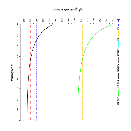
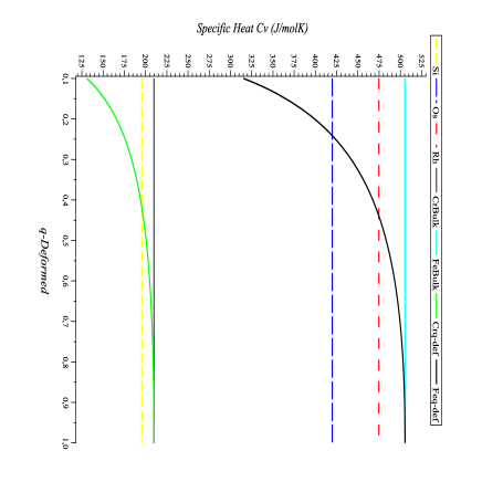
Figure 3: Debye temperature $\theta_{D}$ range of $Fe$ and $Cr$ varying as a function of $q=0.1$ to $q\to 1$ (top); $q$-deformed specific heat $c_{V}$ range of $Fe$ and $Cr$ varying as a function of $q=0.1$ to $q\to 1$ (bottom).

For $T\gg\theta_{D_{q}}$, then $\alpha_{0_{q}}\ll 1$, the function $D(\alpha_{0})_{q}$ can be expressed in a power series in $\alpha_{0_{q}}$

$$D(\alpha_{0})_{q}=1-\frac{\alpha_{0_{q}}^{2}}{20}+\cdots$$ (39)

so that for

$$T\to\infty\;,\qquad c_{V_{q}}\to 3\kappa_{B}.$$ (40)

For $T\ll\theta_{D_{q}}$, then $\alpha_{0_{q}}\gg 1$, we can write function $D(\alpha_{0})_{q}$ as

$$\frac{12}{\alpha_{0_{q}}^{3}}\displaystyle\int_{0}^{\infty}{\frac{\alpha^{3}d\alpha}{\exp(\alpha)-1}+O[\exp(-\alpha_{0_{q}})]},$$ (41)

$$\approx\frac{4\pi^{4}}{5\alpha_{0_{q}}^{3}}=\frac{4\pi^{4}}{5}\left(\frac{T}{\theta_{D_{q}}}\right)^{3}.$$ (42)

Thus, as in the usual Debye solid, low temperature specific heat in a $q$-deformed Debye solid is proportional to $T^{3}$ rather than proportional to the exponential function in (25) for the $q$-deformed Einstein solid. This is in agreement with experiments. Finally, we express the specific heat for low temperatures as

$$c_{V_{q}}=\frac{12\pi^{4}\kappa_{B}}{5}\left(\frac{T}{\theta_{D_{q}}}\right)^{3}=1944\left(\frac{T}{\theta_{D_{q}}}\right)^{3}\frac{J}{molK}.$$ (43)

For the $q$-deformed case one can observe the changes that occur with Debye temperature, specific heat, thermal and electrical conductivies and electric resistivity. By using the relationship established for thermal conductivity $\kappa$ zim we obtain

$$\kappa=\frac{1}{3}C_{V}vl,$$ (44)

where $v$ is the average velocity of the particle, $C_{V}$ is the molar heat capacity and $l$ is the space between particles. We can deduce a relationship between the thermal and electrical $\sigma$ conductivities through the elimination of $l$ (as $\sigma=\frac{ne^{2}l}{mv}$, where $m$ is the electron mass, $n$ is the number of electrons per volume unit and $e$ is the electron charge), such that

$$\frac{\kappa}{\sigma}=\frac{1}{3}\frac{C_{V}mv^{2}}{ne^{2}}.$$ (45)

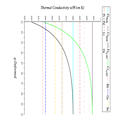
Figure 4: Thermal conductivity $\kappa$ range of $Fe$ and $Cr$ varying as a function of $q=0.1$ to $q\to 1$.

In a classical gas the average energy of a particle is $\frac{1}{2}mv^{2}=\frac{3}{2}\kappa_{B}T$, whereas the heat capacity is $\frac{3}{2}n\kappa_{B}$, so that

$$\frac{\kappa}{\sigma}=\frac{\pi^{2}}{3}\left(\frac{\kappa_{B}}{e}\right)^{2}T$$ (46)

the ratio $\frac{\kappa}{\sigma T}$ is called the Lorenz number and should be a constant, independent of the temperature and of the scattering mechanism. This is the famous Wiedemann-Franz law, which is often well satisfied experimentally, and the Lorenz number correctly given zim .

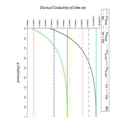
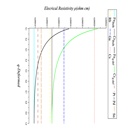
Figure 5: Electrical conductivity $\sigma$ range of $Fe$ and $Cr$ varying as a function of $q=0.1$ to $q\to 1$ (top); electrical resistivity $\rho$ range of $Fe$ and $Cr$ varying as a function of $q=0.1$ to $q\to 1$ (bottom).

By using the $q$-deformed relations presented above, we start from Eqs. (44) and (46) to determine the important relations for $q$-deformed thermal and electrical conductivities

$$\kappa_{q}=\frac{\kappa c_{V_{q}}}{c_{V}}\qquad\qquad\mbox{and}\qquad\qquad\sigma_{q}=\frac{\kappa_{q}\sigma}{\kappa}.$$ (47)

Since electrical resistivity $\rho$ is the inverse of conductivity, $q$-deformed $\rho_{q}=\frac{1}{\sigma_{q}}$. Recall that to compute these deformed quantities in terms of the specific heat $c_{Vq}$ we make use of the equation (37) and its suitable limits. Data is plotted to provide a better view of our results. We see how $q$-deformation is acting on chemical element properties. For illustration purposes, we chose iron (Fe) and chromium (Cr) two materials that can be employed in many areas of interest.

Fig. 3 shows how $q$-deformation acts on $Fe$ and $Cr$ Debye temperatures and specific heat. The plots show that $Fe$ reaches rhodium (Rh) values for $q\approx 0.45$, osmium (Os) for $q\approx 0.25$ while $Cr$ approaches silicon (Si) for $q\approx 0.42$.

Fig. 4 shows that thermal conductivity for $Fe$ approaches the thermal conductivity of rubidium (Rb) for $q\approx 0.15$, whereas $Cr$ equals bulk $Fe$ for $q\approx 0.27$, lithium (Li) for $q\approx 0.35$ and $Os$ for $q\approx 0.48$. They also approach the germanium (Ge) for $q\approx 0.17$ and $q\approx 0.1$, tin (Sn) for $q\approx 0.25$ and $q\approx 0.15$, platinum (Pt) and palladium (Pd) for $q\approx 0.35$ and $q\approx 0.18$, respectively.

Fig. 5 shows that electrical conductivity and resistivity of $Fe$ equals $Ga$ for $q\approx 0.12$, bulk $Cr$ for $q\approx 0.18$, $Rb$ for $q\approx 0.2$, $Sn$ for $q\approx 0.33$, $Pt$ and $Pd$ for $q\approx 0.45$, while $Cr$ equals cesium (Cs) with $q\approx 0.11$ and $Ga$ for $q\approx 0.29$.

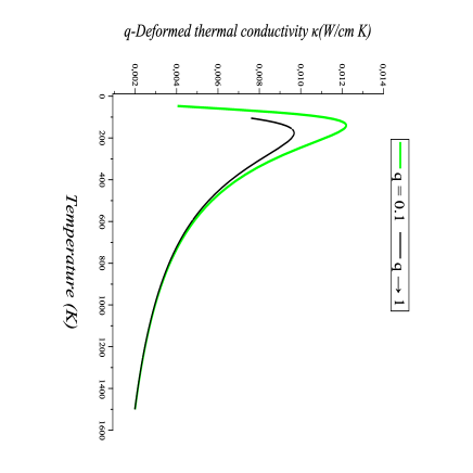
Figure 6: $q$-Deformed thermal conductivity $\kappa_{q}$ for $Cr$ as $q\to 1$ and for $Cr$ with impurities as $q=0.1$ vs temperature $T$, in the interval $T=0$ to $T=1500K$ .

Fig. 6 shows correct behavior of thermal conductivity for a pure and impure material. One should note that $q$-deformation is clearly playing the role of impurity concentration in the material sample. This is because $q$-deformation acts directly on Debye temperature, which means that the Debye frequency is modified. Changing the Debye frequency is a clear sign of the material being modified by impurities.

IV Conclusions

Following our previous results in bri , we understand $q$-deformation not only as a mathematical tool, but also as an impurity factor in a material, such as disorder or reorganization of a crystalline structure.

In the present study, we first investigate the Einstein solid model to obtain thermodynamic quantities such as Einstein temperature, Helmholtz free energy, specific heat and internal energy with $q\neq 1$. We then generalize this study to the Debye solid model to obtain the Debye temperature, specific heat, thermal conductivity, electrical conductivity and resistivity. We present these findings for a number of chemical elements.

Our main results indicate the possibility of adjusting $q$-deformation to obtain desirable physical effects, such as changing the thermal conductivity of a certain element, which might become equivalent to a material that is easier to handle by inserting an impurity in a sample of the original element. We need further studies and evidence to substantiate such a complex hypothesis. For example, we are seeking to establish a connection between this theory and experiments through the growth of thin films, a matter that will be addressed elsewhere.

- (1) A.U. Klimyk, Spectra of Observables in the -Oscillator and -Analogue of the Fourier Transform, Methods and Applications, 1, 8, (2005).
- (2) R. Jaganathan and S. Sinha, J. Phys. Pramana, 3, 64, (2005).
- (3) C. Tsallis, Introduction to Nonextensive Statistical Mechanics - Approaching a Complex World, Springer, New York, (2009).
- (4) L.C. Biedenharn and M.A. Lohe, Quantum Group Symmetry and -Tensor Algebras, World Scientific, Singapore, (1995).
- (5) A. Macfarlane, J. Phys. A: Math. Gen. 22, 4581 (1989).
- (6) E.G. Floratos, J. Phys. Math. 24, 4739 (1991).
- (7) V.V. Borzov, E.V. Damaskinsky, S.B. Yegorov , arXiv:-alg/9509022v1.
- (8) O.F. Dayi, I.H. Duru, arXiv:hep-th/9410186v2.
- (9) F.A. Brito, A.A. Marinho, Physica A 390, 2497-2503 (2011).
- (10) C.Kittel, Introduction to Solid State Physics, John Wiley & Sons, (1996)
- (11) R.K. Patthria, Statistical Mechanics, Pergamon press, Oxford (1972)
- (12) P.W. Anderson, Absence of diffusion in certain random lattices, Phys. Rev. 5, 109 (1958).
- (13) P.A. Lee, T.V. Ramakrishnan, Rev. Mod. Phys. 2, 57 (1985).
- (14) R.J. Elliott et al., Rev. Mod. Phys., 3 46 (1974).
- (15) M. Chaichian, R. Gonzales Felipe, C. Montonen, J. Phys. A: Math. Gen. 26, 4017 (1993).
- (16) Y.J. Ng, J. Phys. A 23, 1023 (1990).
- (17) J.J. Sakurai, Modern Quantum Mechanics, (Late-Univ. of California, LA (1985)).
- (18) L. Biedenharn., J. Phys. A: Math. Gen. 22, L873 (1989).
- (19) T. Ernst, The History of -calculus and a new method. (Dep. Math., Uppsala Univ. 1999-2000).
- (20) F.H. Jackson, Trans. Roy Soc. Edin. 46, 253-281 (1908).
- (21) F.H. Jackson, Mess. Math. 38, 57 (1909).
- (22) A. Lavagno and N.P. Swamy, Phys. Rev. E 61, 1218 (2000); A. Lavagno and N.P. Swamy, Phys. Rev. E 65, 036101 (2002).
- (23) F. Reif, Fundamentals of statistical and thermal physics, Tokyo, (1965).
- (24) K. Huang, Statistical Mechanics, John Wiley & Sons, (1987).
- (25) J.M. Ziman, Electron and Phonons - The Theory of Transport Phenomena in Solids, Oxford Univ. Press, (1960).