Discrete Wigner Function Reconstruction and Compressed Sensing

Abstract

A new reconstruction method for Wigner function is reported for quantum tomography based on compressed sensing. By analogy with computed tomography, Wigner functions for some quantum states can be reconstructed with less measurements utilizing this compressed sensing based method.

Wigner function(WF), a quasi-probability distribution in phase space, was first introduced to describe quantum state in quantum mechanics by E. P. Wignerwigner . And later, it was extended to classical optics and signal processing. Since its birth, a great number of applications have been conducted in different fields. As for the original quantum case, like a continuous one-dimensional quantum system, the Wigner function is defined as

$$W(x,p)\equiv\frac{1}{\pi}\int_{-\infty}^{\infty}d\xi\exp(-2ip\xi)\langle x+\xi|\hat{\rho}|x-\xi\rangle$$ (1)

where $x$ and $\xi$ are positions and $p$ is momentum, $\hat{\rho}$ denotes the density operator, and $\hbar$ is set to 1 for simplicity.

One of the advantage for the Wigner formalism is that a tomographic scheme which could be used to reconstruct the WF. On the other hand, in medical tomography, like X-ray computed tomography, X-ray photons transmitted through the patient along projection lines from one side, and detectors measured the number of transmitted photons on the other side, then from the distribution of X-ray photons in different incident angles, linear attenuation coefficients in the slice being imaged are recovered. Likewise, in phase space tomography, the WF tomographic reconstruction is more or less the same, based on a set of intensity measurementsvogelpra . This is because both of the two tomographic schemes share the same mathematical basis — Radon transform(Eqn.(2)) and its inverse(Eqn.(3)).

$$pr(x_{\phi},\phi)=\int\int f(x,y)\delta(x_{\phi}-x\cos\phi-y\sin\phi)dxdy$$ (2)

$$f(x,y)=-\frac{1P}{2\pi^{2}}\int_{0}^{\pi}\int_{-\infty}^{+\infty}\frac{pr(x_{\phi},\phi)dx_{\phi}d\phi}{(x\cos\phi+y\sin\phi-x_{\phi})^{2}}$$ (3)

Where $P$ denotes the Cauchy’s principle value, $pr(x_{\phi},\phi)$ denotes the measured distribution, in $f(x,y)$ is the quantity in tomography to be recovered. In tomography, objective function is reconstructed using back-projection algorithm for the inverse Radon transformation(Eqn.(3)). However, such a algorithm has some drawbacks, for example, many measurements are needed to achieve a relatively good recovery. To reduce the dose of radiation on the patient in CT or make a more efficient estimate of quantum state in phase space tomography, the amount of measurements should be as small as possible but guarantee a good enough recovery. Nevertheless, according to the well-known Nyquist-Shannon sampling theoremunser , it seems impossible to depress the measurements without giving a negative impact on the resolution.

Recently, with the arise of a novel theory called compressed sensing (compressive sampling or CS) candes , people find a fundamentally new approach to acquire data. It demonstrates that if the images or signals are sparse, we can recover them from what was believed to be highly incomplete measurements. In fact, it is just the application to medical tomography that started the seminal paper in CS. For example, in CT, X-ray images of human body are sparse in the wavelet and gradient representation, then compressed sensing is applied to reduce the irradiation and obtain clearer medical imagessidky ; Chen . And then an immediate question would be is it possible to reconstruct WF in phase space tomography via compressed sensing? In fact, there exists infinite family of quasi-probability distribution in phase, including Husimi-Kando Q-Function, Glauber-Sudarshan P-Function and so on, but WF is chose for it is directly related to the quadrature histograms and can be easily measured through experiments.

In this brief report, we explore the similarity between phase space tomography and computed tomography, and report a new discrete WF reconstruction method based on compressed sensing. We mention that some compressed sensing protocols have been proposed to reconstruct density matrix though quantum tomographyGrossprl .

Suppose that a signal $x\in\mathbb{C}^{N}$ is sparse in some basis $x=\Psi x^{\prime}$, which means $x^{\prime}$ has $k(k\ll N)$ nonzero entries. Then a measurement matrix $\Phi\in\mathbb{C}^{m\times N}$ is used to sense $x$ and obtain a measurement vector $y\in\mathbb{C}^{m}$. The central idea of compressed sensing is that it is possible to reconstruct sparse signals of scientific interest accurately and sometimes exactly by a number of incoherent sampling which is far smaller than N. In general, such a recovery of $x$ by performing $\ell_{0}$-minimization is a NP-hard problem. An alternative procedure called $\ell_{1}$-minimization is usually used which says

$$\min_{x^{\prime}}\|x^{\prime}\|_{\ell_{1}}\qquad\textrm{subject to}\qquad y=\Phi\Psi x^{\prime}=\Upsilon x^{\prime},$$ (4)

This is a convex optimization problem, and many numerical algorithms apply for its solution.

Before showing the reconstruction method, we note that there are two main differences between conventional medical tomography and the quantum tomography. First, WF is a pseudo probability distribution, may have negative values, while the attenuation coefficients in CT images are always nonnegative. Second, for a given angle, a complete probability density for the quadrature operator is measured due to the quantum mechanical property, but in medical tomography, detectors’ number can be adjusted. On the other hand, similar to the medical case, at the heart of a possible CS application to phase space tomography is to find a suitable sparse representation basis. In real computed tomography, images are generally extended distributions which violate the prerequisite of $\ell_{1}$-based algorithms. But other sparseness property (gradient sparse) and reconstruction algorithm(TV-algorithm)sidky are found to reconstruct certain tomographic images which are relatively constant over extended areas. While due to its configuration’s flexibility , it is hard even impossible to find a unitive sparse basis for WF in general. However, for some special applications, WF might share the same sparse basis. And in contrary to the medical images, some quantum states have finite values on a small region in phase space with zero or nearly zero values elsewhere, so have been sparse in this pseudo-pixel representation. Other situations may be completely different, for WF is not sparse in phase space representation. A basis transform like Fourier transform, wavelet transform may bring WF to a sparse representation.

Although it is also possible to reconstruct continuous Wigner function, but discretization must be taken before it can be tackled in practise. So in this report we adopt a discrete quantum tomography model. But we note that it should be straightforward to transport our idea to an continuous one. And indeed such an attempt has been taken in information scienceChen . The quantum state tomographic model for discrete Wigner functions first proposed by U. Leonhardtleonhardt . We note that continuous and discrete quantum tomography are the same in principle. In finite quantum systems, position and momentum take discrete values in $\mathbb{Z}_{d}$. In Leonhardt’s discrete quantum tomography picture, a WF in a $d$-dimensional(odd) Hilbert space was proposed(Eqn.(6)) and phase was quantized to take place of momentum in continuous variable quantum systems.

$$W(m,\mu)=\frac{1}{d}\sum_{n}\exp(-\frac{4\pi i}{d}\mu n)\langle m-n|\hat{\rho}|m+n\rangle$$ (5)

Here, $m,n$ denotes the spins or particle numbers, $\mu,\nu$ denotes the quantized phases. Similar to the continuous case, the observable distribution is the overlap of measured state’s WF and the observable state’s WF in phase space.

$$pr(\mu_{0},\tau)=\sum_{\mu,m}W(m,\mu)\delta(\mu-\mu_{0}+2m\tau;d)$$

$$pr(m_{0},\tau)=\sum_{\mu,m}W(m,\mu)\delta(m-m_{0};d)\delta(m-m_{0};a).$$ (6)

Here, $m_{0},\mu_{0}\in\mathbb{Z}_{d},pr(\mu_{0},\tau)$ denotes the probability distribution, $W(m,\mu)$ denotes the WF to be recovered, $\tau\in\mathbb{Z}_{d}$, $m,m_{0}$ represent the spins or particle numbers, $\mu,\mu_{0}$ represent the quantum phases and $\delta(k;a)$ is the modular Kronecker symbol(equals 1 when $k$=0 (mod a), and zero otherwise)

In our simulation, a WF for finite dimensional coherent state $||\alpha|\textrm{e}^{i\phi}\rangle_{s}$ (s=d-1)Miranowicz is used as an example to illustrate the CS based reconstruction algorithm.

$$W(m,\mu) = \sum_{k=M+1}^{s}$$ (7)

$$\times \frac{\exp[i(2k-M-s-1)(2\pi\mu/d-\phi+\pi/2)]}{[k!(M-k-s-1)!]^{1/2}}G_{1k}$$

$$+ \sum_{k=0}^{M}\frac{\exp[i(2k-M)(2\pi\mu/d-\phi+\pi/2)]}{[k!(M-k)!]^{1/2}}G_{0k}$$

where

$$G_{\eta k} = \frac{(s!)^{2}}{(s+1)^{3}}\sum_{p=0}^{s}\sum_{q=0}^{s}$$

$$\times \exp[i(x_{q}-x_{p})|\alpha|]\frac{\textrm{He}_{k}(x_{p})\textrm{He}_{M-k+\eta(s+1)}(x_{q})}{[\textrm{He}_{s}(x_{p})\textrm{He}_{s}(x_{q})]^{2}}$$

with $\eta=0,1$, $M\equiv 2n\textrm{mod}(d)$, $\textrm{He}_{s+1}(x)$ is the Hermite polynomial ($\textrm{He}_{n}(x)\equiv 2^{-n/2}H_{n}(x/\sqrt{2})$) and $x_{k}$ is the $k$th root of $\textrm{He}_{s+1}(x)=0$.

It should be pointed out that different from classical signal processing (the sensing matrix elements can be independently selected from a random distribution), only the rows of the sensing matrix can be randomly measured in quantum tomography. The sensing matrix was randomly selected from the rows of full measurement matrix (modular Kronecker in Eqn.(7)). Then, we get the precise probability distribution by multiplying the sensing matrix and the WF. The problem considered now is to reconstruct a state from measured insufficient data. Computer simulation has been conducted to demonstrate the effectiveness of the aforementioned scheme. All the recovery processes were implemented in Java and C. For $\ell_{1}$-minimization, we adopt a linearized bergman iteration algorithmyin .

To simulate the sampling process, we assign a number to each row of the full measurement matrix, then computer generated a series of random numbers representing the rows we select to form the sensing matrix. For simplicity, the experiment error was totally ignored. So in this pseudo pixel representation, WF can be just roughly reconstructed. This is partly due to measurement process itself, for only a small fraction of the WF is sensed once, which means the sensing matrix is not dense enough. To overcome this obstacle, two approaches might help: finding another sparse representation or using a denser sensing matrix(measurement quantum state, for example, coherent state). For example, for some type of mixed state ensemble, WF varies along a particular direction when we rearrange the two dimensional WF into a one dimensional object carefully, it is sparse in a discrete cosine Fourier representation, which means this basis is its sparse basis.

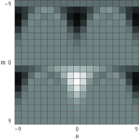
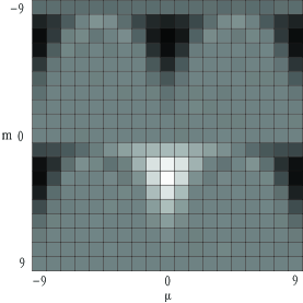
FIG. 1: Darker regions correspond to higher values, the regions between dark and white are dominated by zero or nearly zero values .(a)Accurate WF for finite dimensional coherent state(Eqn.(8), $d=19$, $|\alpha=1.472\rangle$). (b) Recovered WF via compressed sensing, 285 rows have been taken from total measurement matrix as the sensing matrix.

In spite of some drawbacks, when we deal with a high dimensional quantum state reconstruction or what we need is just a rough knowledge of WF, our reconstruction algorithm would show its advantage, it makes the measurements more economical. And any other prior knowledge could also be helpful to recovery process, for example, the symmetry of the WF. By exploring the correspondence between compressed sensing and tomography, we have shown the possibility of a CS-based WF reconstruction method. In addition, most convex optimization algorithms related to CS theory deal with real signal. And in our case, WF is real function. But when we need to reconstruct complex signals or images, for example, ambiguity function(AF)testorf which is complex in general, problems appear. Here, we mention that G.Zweig proposed an algorithmzweig processing complex signals, which converted the the usual $\ell_{1}$-minimization in complex space to a linear programming problem in real space.

In conclusion, we have described a reconstruction method based on compressed sensing to recover the WF in phase space tomography. We regard the Wigner function as an image in phase space. The values of WF on different sites corresponds to pixels’ gray values. Our numerical simulation has shown good recovery for a sparse discrete WF with usually supposed insufficient measurements. Such a method can also be easily extended to reconstruct electromagnetic field’s WF with just some straightforward revisions. We hope that our scheme can serve as a motivation for other quantum information or phase space optics researches. Possible relations to the popular maximum-likelihood reconstruction in quantum tomography still need to be explored. By combination with other reconstruction ideas, we believe a more efficient and precise phase recovery should be possible.

This work is supported by the NSF of China(Grant No. 11075077) and also partly by the SRFDP of China(Grant No. 200800550015).

References

- (1) E. P. Wigner, Phys. Rev. 40 749 (1932).
- (2) K. Vogel, and H. Risken, Phys. Rev. A 40 2847 (1989).
- (3) M. Unser, Proc. IEEE 88 569 (2000).
-
(4)
D. Donoho, IEEE Trans. Inf. Theory 52 1289 (2006).
E. J. Candès, J. Romberg, and T. Tao, Comm. Pure Appl. Math. 59 1207 (2006); - (5) E. Y. Sidky, C.-M.Kao, and X. Pan, J. X-ray Sci. Tech. 14 119 (2006)
- (6) G. H. Chen, J. Tang, and S. Leng, Med. Phys. 35 660 (2008)
- (7) D. Gross, Y.-K.Liu, S. T. Flammia, S. Becker, and J. Eisert Phys. Rev. Lett. 105 150401 (2010).
- (8) D. T. Smithey, M. Beck, M. G. Raymer, A. Faridani, Phys. Rev. Lett. 70 1244 (1993).
- (9) A. I. Lvovsky, and M. G. Raymer, Rev. Mod. Phys. 81 299 (2009).
- (10) P. Flandrin, P. Borgnat IEEE Trans. Signal Process. 58 2974 (2010).
- (11) U. Leonhardt Phys. Rev. Lett. 74 4101 (1995).
- (12) A. Miranowicz, W. Leonski and N. Imoto Adv. Chem. Phys. 119 155 (2001).
- (13) W. Yin, S. Osher, D. Goldfarb, and J. Darbon, J. Imaging Sci. 1 143 (2008)
- (14) M. Testorf, B. M. Hennelly and J. Ojeda-Castaneda, Phase-Space Optics: Fundamentals and Application McGraw-Hill, New York, 2009.
- (15) G. Zweig, IEE Proc.-Radar Sonar Navig. 150 247 (2003).