Transportation dynamics on networks of mobile agents

Abstract

Most existing works on transportation dynamics focus on networks of a fixed structure, but networks whose nodes are mobile have become widespread, such as cell-phone networks. We introduce a model to explore the basic physics of transportation on mobile networks. Of particular interest are the dependence of the throughput on the speed of agent movement and communication range. Our computations reveal a hierarchical dependence for the former while, for the latter, we find an algebraic power law between the throughput and the communication range with an exponent determined by the speed. We develop a physical theory based on the Fokker-Planck equation to explain these phenomena. Our findings provide insights into complex transportation dynamics arising commonly in natural and engineering systems.

I Introduction

Transportation processes are common in complex natural and engineering systems, examples of which include transmission of data packets on the Internet, public transportation systems, migration of carbon in biosystems, and virus propagation in social and ecosystems. In the past decade, transportation dynamics have been studied extensively in the framework of complex networks ASG:2001 ; KYHJ:2002 ; TB:2004 ; TTR:2004 ; MB:2004 ; PLZY:2005 ; SG:2005 ; CLLF:2005 ; DYMB:2006 ; LRMHSA:2010 , where a phenomenon of main interest is the transition from free flow to traffic congestion. For example, it is of both basic and practical interest to understand the effect of network structure and routing protocols on the emergence of congestion ZLPY:2005 ; WWYXZ:2006 ; ZLRH:2007 ; GKL:2008 ; yang2008 ; TLLH:2009 ; LHJWCW:2009 ; TM:2009 ; XWLHH:2010 . Despite these works, relatively little attention has been paid to the role of individual mobility. The purpose of this paper is to address how this mobility affects the emergence of congestion in transportation dynamics.

The issue of individual mobility has become increasingly fundamental due to the widespread use of ad-hoc wireless communication networks. The issue is also important in other contexts such as the emergence of cooperation among individuals HY:2009 and species coexistence in cyclic competing games RMF:2007 . Recently, some empirical data of human movements have been collected and analyzed HBG:2006 ; GHB:2008 . From the standpoint of complex networks, when individuals (nodes, agents) are mobile, the edges in the network are no longer fixed, requiring different strategies to investigate the dynamics on such networks than those for networks with fixed topology. In this paper, we shall introduce an intuitive but physically reasonable model to deal with transportation dynamics on such mobile/non-stationary networks. In particular, we assume in our model that communication between two agents is possible only when their geographical distance is less than a pre-defined value, such as the case in wireless communication. Information packets are transmitted from their sources to destinations through this scheme. To be concrete, we assume the physical region of interest is a square in the plane, and we focus on how the communication radius and moving speed may affect the transportation dynamics in terms of the emergence of congestion. Our main results are the following. Firstly, we find that congestion can occur for small communication range, limited forwarding capability and low mobile velocity of agents. Secondly, the transportation throughput exhibits a hierarchical structure with respect to the moving speed and there is in fact an algebraic power law between the throughput and the communication radius, where the power exponent tends to assume a smaller value for higher moving speed. To explain these phenomena in a quantitative manner, we develop a physical theory based on solutions to the Fokker-Planck equation under initial and boundary conditions that are specifically suited with the transportation dynamics on mobile-agent networks. Besides providing insights into issues in complex dynamical systems such as contact process, random-walk theory, and self-organized dynamics, our results will have direct applications in systems of tremendous importance such as ad-hoc communication networks MAHN4 ; MAHN6 ; MAHN7 .

In Sec. II, we describe our model of mobile agents in terms of the transportation rule and the network structure. In Sec. III, we present numerical results on the order parameter, the critical transition point and the average hopping time. In Sec. IV, a physical theory is presented to explain the numerical results. A brief conclusion is presented in Sec. V.

II Transportation rule and network structure of mobile agents

In our model, $N$ agents move on a square-shaped cell of size $L$ with periodic boundary conditions. Agents change their directions of motion $\theta$ as time evolves, but the moving speed $v$ is the same for all agents. Initially, agents are randomly distributed on the cell. After each time step, the position and moving direction of an arbitrary agent $i$ are updated according to

$$x_{i}(t+1)=x_{i}(t)+v\cos\theta_{i}(t),$$ (1)

$$y_{i}(t+1)=y_{i}(t)+v\sin\theta_{i}(t),$$ (2)

$$\theta_{i}(t)=\Psi_{i},$$ (3)

where $x_{i}(t)$ and $y_{i}(t)$ are the coordinates of the agent at time $t$, and $\Psi_{i}$ is an $N$-independent random variable uniformly distributed in the interval $[-\pi,\pi]$. Each agent has the same communication radius $a$. Two agents can communicate with each other if the distance between them is less than $a$. At each time step, there are $R$ packets generated in the system, with randomly chosen source and destination agents, and each agent can deliver at most $C$ packet (we set $C=1$ in this paper) toward its destination. To transport a packet, an agent performs a local search within a circle of radius $a$. If the packet’s destination is found within the searched area, it will be delivered directly to the destination and the packet will be removed immediately. Otherwise, the packet is forwarded to a randomly chosen agent in the searched area. The queue length of each agent is assumed to be unlimited and the first-in-first-out principle holds for the queue. The transportation process is schematically illustrated in Fig. 1.

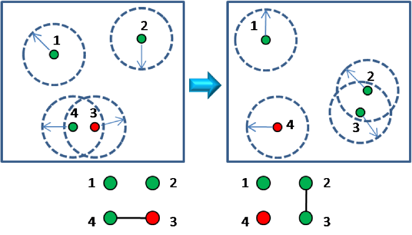
Figure 1: (Color online) Schematic illustration of transportation process among mobile agents. The dashed circles denote the communication range, the arrows denote the moving directions, and each agent is specified by a number. Agents without data packets are in green (light gray) and agents holding data packets are in red (dark gray). In the left panel, agent 3 and 4 can communicate with each other, where the former holds a packet. Agent 3 delivers the packet to agent 4 and then all agents move, as shown in the right panel. After the movements, all agents randomly set new directions. There can be more than one agent in the communication range of any agent. The relevant communication networks are shown in the bottom.

The communication network among the mobile agents can be extracted as follows. Every agent is regarded as a node of the network and a wireless link is established between two agents if their geographical distance is less than the communication radius $a$. Due to the movement of agents, the network’s structure evolves from time to time. The network evolution as a result of local mobility of agents is analogous to a locally rewiring process. As shown in Fig. 1, nodes 1 and 2 are disconnected while node 3 and node 4 are connected at time $t$. At time $t+1$, nodes 1 and 2 depart from each other and become disconnected while nodes 3 and 4 approach each other and establish a communication link. Note that the mobile process does not hold the same number of links at different time, which is different from the standard rewiring process where the number of links is usually fixed.

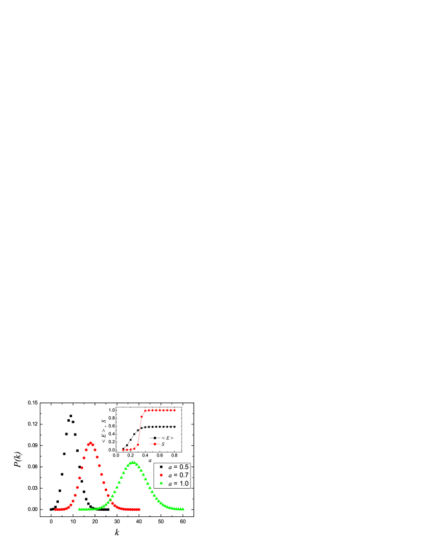
Figure 2: (Color online) The proportion of nodes $P(k)$ as a function of degree $k$ for different communication radius $a$. The inset shows that the relative size $S$ of the largest connected component and the clustering coefficient $\langle E\rangle$ as a function of communication radius $a$. The number of agents is 1200 and the size of the square region is $L=10$.

We define an agent’s degree at a specific time step as the number of links at that moment. Figure 2 shows that the degree distribution of networks of mobile agents exhibits the Poisson distribution:

$$P(k)=\frac{e^{-\langle k\rangle}\langle k\rangle^{k}}{k!},$$ (4)

where $k$ is the degree, $P(k)$ is the proportion of nodes with degree $k$ and $\langle k\rangle$ is the average degree of network. As shown in Fig. 2, the average degree $\langle k\rangle$ increases as the communication radius $a$ increases and the peak value of $P(k)$ decreases as $a$ increases. We also investigate the relative size of the largest connected component and the clustering properties of the network in terms of the clustering coefficient. The relative size $S$ of the largest connected component is defined as

$$S=\frac{S_{1}}{N},$$ (5)

where $S_{1}$ and $N$ is the size of the largest connected component and the total network respectively. The clustering coefficient $E_{i}$ for node $i$ is defined as the ratio between the number of edges $e_{i}$ among the $k_{i}$ neighbors of node $i$ and its maximum possible value, $k_{i}(k_{i}-1)/2$, i.e.,

$$E_{i}=\frac{2e_{i}}{k_{i}(k_{i}-1)}.$$ (6)

The average clustering coefficient $\langle E\rangle$ is the average of $E_{i}$ over all nodes in the network. The insert of Fig. 2 shows that $S$ and $\langle E\rangle$ increase as the communication radius $a$ increases. In particular, when the value of $a$ exceeds a certain value. e.g., $0.4$, high values of $S$ and $\langle E\rangle$ is attained. We also note that the motion speed does not influence the statistical properties of the communication network. In general, the communication network caused by limited searching area and mobile behavior is of geographically local connections associated with Poisson distribution of node degrees and dense clustering structures.

III Numerical results

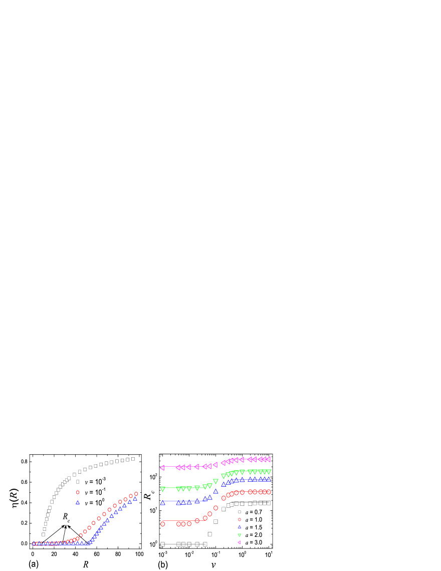
Figure 3: (Color online) (a) Order parameter $\eta(R)$ versus $R$ for different values of speed $v$ and (b) dependence of the critical $R_{c}$ on $v$ for different communication radius $a$. The number of agents is 1200 and the size of the square region is $L=10$. The delivery capacity $C$ of each agent is set to be unity. In (a), $a=1.2$ and $\eta(R)$ is obtained by averaging over $10^{5}$ time steps after disregarding $2\times 10^{4}$ initial steps as transients. The results in both (a) and (b) are obtained by an ensemble average of 20 independent realizations. The lines in (b) are theoretical prediction from Eqs. (26) and (28).

To characterize the throughput of a network, we exploit the order parameter $\eta$ introduced in Ref. ASG:2001 :

$$\eta(R)=\lim_{t\rightarrow\infty}\frac{C}{R}\frac{\langle\Delta N_{p}\rangle}{\Delta t},$$ (7)

where $\Delta N_{p}=N_{p}(t+\Delta t)-N_{p}(t)$, $\langle\cdot\cdot\cdot\rangle$ indicates the average over a time window of width $\Delta t$, and $N_{p}(t)$ represents the total number of data packets in the whole network at time $t$. As the packet-generation rate $R$ is increased through a critical value of $R_{c}$, a transition occurs from free flow to congestion. For $R\leq R_{c}$, due to the absence of congestion, there is a balance between the number of generated and that of removed packets so that $\langle\Delta N_{p}\rangle=0$, leading to $\eta(R)=0$. In contrast, for $R>R_{c}$, congestion occurs and packets will accumulate at some agents, resulting in a positive value of $\eta(R)$. The traffic throughput of the system can thus be characterized by the critical value $R_{c}$ which is on average the largest number of generated packets that can be handled at each time without congestion.

Figure 3(a) exemplifies the transition in the order parameter $\eta(R)$ from free flow to congestion state at some critical value $R_{c}$. We find that $R_{c}$ depends on both the moving speed $v$ and the communication radius $a$. Figure 3(b) shows the dependence of $R_{c}$ on $v$ for different values of $a$. We observe a hierarchical structure in the dependence. Specifically, when $v$ is less or larger than some values, $R_{c}$ remains unchanged at a low and a high value, respectively, regardless of the values of $v$. The transition between these two values of $R_{c}$ is continuous. The hierarchical structure can in fact be predicted theoretically in a quantitative manner (to be described). Figure 4(a) shows the dependence of $R_{c}$ on $a$ for different values of $v$, which indicates an algebraic power law: $R_{c}\sim a^{\beta}$, where $\beta$ is the power-law exponent. We find that the power law holds for a wide range of $a$ and the exponent $\beta$ is inversely correlated with $v$. For example, for $v=0$, $\beta\approx 3.5$ but for large values of $v$, say $v=5$, we have $\beta\approx 2$. When $a$ reaches the size of the square cell, $R_{c}$ is close to $N$ as every agent always stays in the searching range of all others and almost all packets can arrive at their destinations in a single time step.

To gain additional insights into the dependence of $R_{c}$ on the parameters $a$ and $v$ so as to facilitate the development of a physical theory, we explore an alternative quantity, the average hopping time $\langle T\rangle$ in the free flow state which, for a data packet, is defined as the number of hops from its source to destination. As we will see, $\langle T\rangle$ can not only be calculated numerically, it is also amenable to theoretical analysis, providing key insights into the theory for $R_{c}$. Representative numerical results for $\langle T\rangle$ are shown in Fig. 4(b). We see that for large $v$, $\langle T\rangle$ scales with $a$ as $a^{-2}$ and, as both $v$ and $a$ are increased, $\langle T\rangle$ decreases.

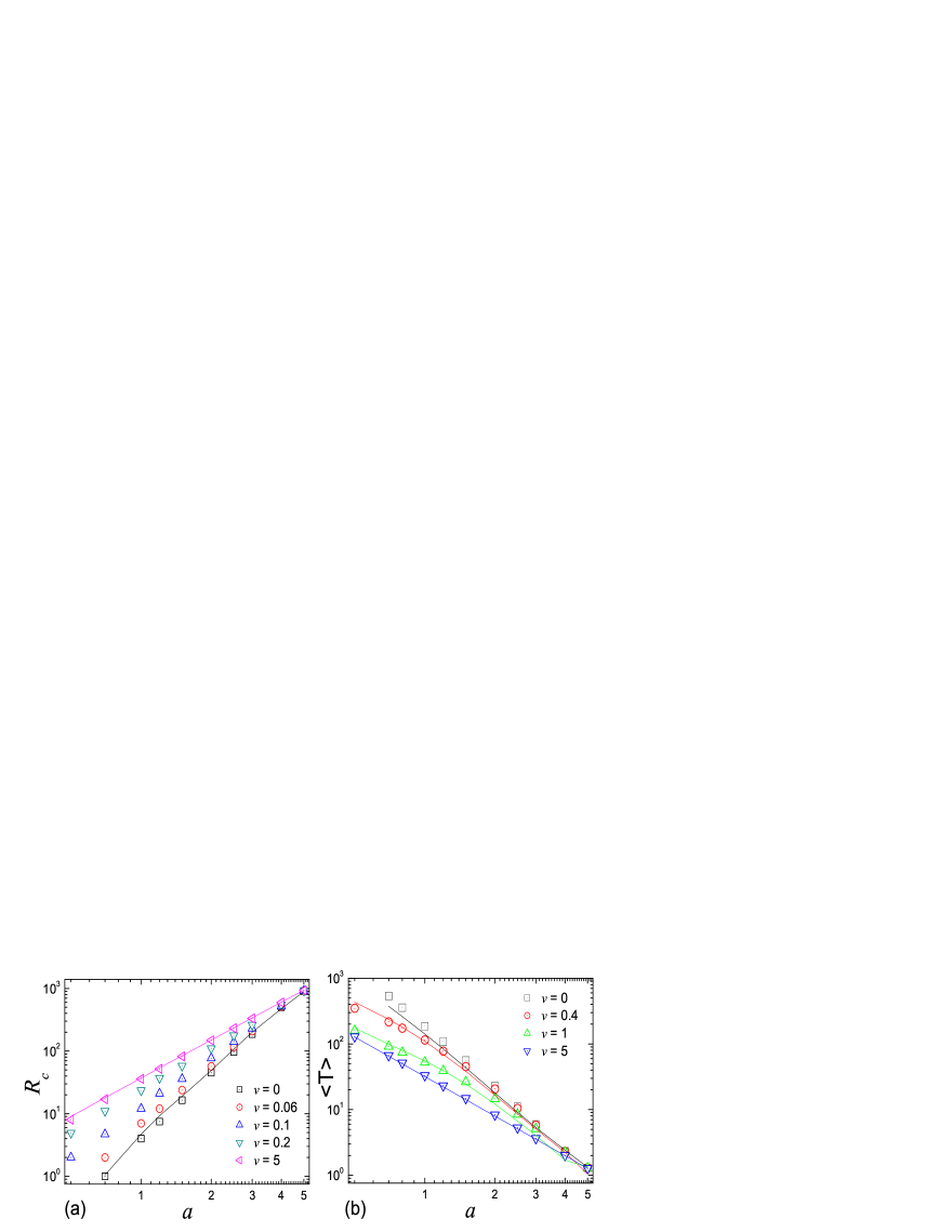
Figure 4: (Color online) (a) Critical value $R_{c}$ as a function of the communication radius $a$ for different values of $v$. The lines are theoretical predictions from Eqs. (26) and (28). (b) Average hopping time $\langle T\rangle$ as a function of $a$ for different values of $v$. The theoretical curves are obtained from Eqs. (20)-(23). For $v=0.4$ and $v=1$, $f=1$ is used. The average time is computed in the free flow state. Each data point is obtained by averaging over 20 independent realizations.

IV Theory

We now present a physical theory to explain the power law behaviors associated with $\langle T\rangle$ and then $R_{c}$. A starting point is to examine the limiting case of $v=0$, where $\langle T\rangle$ can be estimated analytically. In particular, assume that a particle walks randomly on an infinite plane. There are many holes of radius $a$ on the plane. Holes form a phalanx and the distance between two nearby holes is $L$. The particle will stop walking when it falls in a hole. The underlying Fokker-Planck equation is

$$\frac{\partial P(\textbf{r},t)}{\partial t}=[A\nabla^{2}+U(\textbf{r})]P(\textbf{r},t),$$ (8)

where $P(\textbf{r},t)$ is the probability density function of a particle at location r at time $t$, $A$ is the diffusion coefficient, $U(\textbf{r})$ is the potential energy, $U(\textbf{r})=-\infty$ inside holes and $U(\textbf{r})=0$ outside holes, and $P(\textbf{r},t)=0$ inside holes and $P(\textbf{r},t)>0$ outside holes. Making use of solutions to the eigenvalue problem:

$$[A\nabla^{2}+U(\textbf{r})]\Phi_{n}(\textbf{r})=-\lambda_{n}\Phi_{n}(\textbf{r}),$$ (9)

where $\Phi_{n}(\textbf{r})$ is the normalized eigenfunction and $\lambda_{n}$ is the corresponding eigenvalue, we can expand $P(\textbf{r},t)$ as

$$P(\textbf{r},t)=\sum_{n=1}^{\infty}c_{n}e^{-\lambda_{n}t}\Phi_{n}(\textbf{r}),$$ (10)

where $c_{n}=\int P(\textbf{r},0)\Phi_{n}(\textbf{r})d\textbf{r}$ and the initial probability density $P(\textbf{r},0)$ is distributed over a region of a typical size $a$. The probability that a particle still walks at time $t$ is:

$$Q(t)=\int P(\textbf{r},t)d\textbf{r}=\sum_{n=1}^{\infty}c_{n}d_{n}e^{-\lambda_{n}t},$$ (11)

where $d_{n}=\int\Phi_{n}(\textbf{r})d\textbf{r}$. Since the $n=1$ term is dominant, we have

$$Q(t)\approx c_{1}d_{1}e^{-\lambda_{1}t},$$ (12)

which gives the average hopping time as

$$\langle T\rangle\approx\frac{1}{\lambda_{1}}.$$ (13)

Since

$$\Phi_{1}(x,y)=\Phi_{1}(x+L,y)=\Phi_{1}(x,y+L),$$ (14)

the infinite-plane problem can be transformed into a problem on torus:

$$\nabla^{2}\Phi_{1}(r)=-h^{2}\Phi_{1}(r),\ \ \mbox{for}\ \ a<r<b,$$

$$\Phi_{1}(r=a)=0,\Phi_{1}^{\prime}(r=b)=0,$$ (15)

where $b=L/\sqrt{\pi}$ and

$$\Phi_{1}(r)=B_{1}J_{0}(hr)+B_{2}N_{0}(hr).$$ (16)

$J_{0}$ and $N_{0}$ are the first-kind and the second-kind Bessel Function, respectively, and $B_{2}=-B_{1}J_{0}(ha)/N_{0}(ha)$. The quantity $h$ can be obtained by

$$\frac{J_{0}^{\prime}(hb)}{J_{0}(ha)}=\frac{N_{0}^{\prime}(hb)}{N_{0}(ha)}.$$ (17)

Using

$$J_{0}(x)\approx 1-\frac{x^{2}}{4}+\frac{x^{4}}{64},$$ (18)

$$N_{0}(x)\approx\frac{2}{\pi}[(\ln{\frac{x}{2}}+0.5772)(1-\frac{x^{2}}{4}+\frac{x^{4}}{64})+\frac{x^{2}}{4}-\frac{3x^{4}}{128}],$$ (19)

and combining Eqs. (9) and (IV), we get $\lambda_{1}=Ah^{2}$. For $\Delta t=1$, $\langle(\Delta r)^{2}\rangle=a^{2}/2$, we have $A=\langle(\Delta r)^{2}\rangle/4=a^{2}/8$ and $\lambda_{1}=Ah^{2}=a^{2}h^{2}/8$. Finally, we obtain $\langle T\rangle$ as

$$\langle T\rangle\approx\frac{1}{\lambda_{1}}=\frac{8}{a^{2}h^{2}}.$$ (20)

For $v>0$, $P(\textbf{r},t)$ becomes zero in the area where a hole moves and $Q(t)$ decays with time under two mechanisms: diffusion at rate $\lambda_{1}$ and motion of holes at the rate $\lambda_{w}$. Thus, we have

$$\langle T\rangle\approx\frac{1}{f\lambda_{1}+\lambda_{w}},$$ (21)

where $f$ is the weighting factor ($0\leq f\leq 1$) that decreases as $v$ increases. Specifically, $f=1$ for small $v$ and $f=0$ for large $v$. The quantity $\lambda_{w}$ is given by

$$\hbox{(i)}\ \ \lambda_{w} = \frac{\int_{a}^{v_{s}+a}r\Phi_{1}(r)\arccos(\frac{r^{2}+v_{s}^{2}-a^{2}}{2rv_{s}})dr}{\pi\int_{a}^{b}r\Phi_{1}(r)dr},$$

$$\hbox{(ii)}\ \ \lambda_{w} = \frac{\int_{v_{s}-a}^{v_{s}+a}r\Phi_{1}(r)\arccos(\frac{r^{2}+v_{s}^{2}-a^{2}}{2rv_{s}})dr}{\pi\int_{a}^{b}r\Phi_{1}(r)dr},$$

$$\hbox{(iii)}\ \ \lambda_{w} = \frac{a^{2}}{b^{2}}=\frac{\pi a^{2}}{L^{2}},$$ (22)

where $v_{s}=\sqrt{\langle|\textbf{v}_{1}-\textbf{v}_{2}|^{2}\rangle}=\sqrt{2}v$, (i) is valid for $0<v_{s}<2a<b-a$ or $0<v_{s}<b-a<2a$, (ii) is valid for $2a<v_{s}<b-a$ and (iii) is for $v_{s}>b-a$. For large values of $v$, agents are approximately well-mixed so that we can intuitively expect the average time $\langle T\rangle$ to be determined by the inverse of the ratio of the agent’s searching area and the area of the cell:

$$\langle T\rangle\approx\frac{L^{2}}{\pi a^{2}}.$$ (23)

The validity of this equation is supported by the fact that the ratio of the two areas is equivalent to the ratio of the total number of agents to the number of agents within the searching area. The estimation of $\langle T\rangle$ for large $v$ is consistent with the theoretical prediction from Eqs. (21) and (22)(iii) by inserting $f=0$. The theoretical prediction is in good agreement with simulation results, as shown in Fig. 4(b).

With the aid of Eqs. (20) and (23) for $\langle T\rangle$, we can derive a power law for $R_{c}$. In a free-flow state, the number of disposed packets is the same as that of generated packets $Rt$ in a time interval $t$. For $v=0$, the number of packets $n_{i}$ passing through an agent is proportional to its degree. This yields

$$n_{i}=\frac{R\langle T\rangle tk_{i}}{\Sigma_{j}k_{j}}=\frac{R\langle T\rangle tk_{i}}{N\langle k\rangle},$$ (24)

where $k_{i}$ is the degree of $i$, the sum runs over all agents in the network, and $\langle k\rangle$ is the average degree of the network. During $t$ steps, an agent can deliver at most $C_{i}t$ packets. To avoid congestion requires $n_{i}\leq C_{i}t$. If all agents have the same delivering capacity $C$, the transportation dynamics is dominated by the agent with the largest number of neighbors and the transition point $R_{c}$ can be estimated by

$$\frac{R_{c}\langle T\rangle tk_{max}}{N\langle k\rangle}=Ct,$$ (25)

where $k_{max}$ is the largest degree of the network. Thus, for $v=0$, we have

$$R_{c}=\frac{NC\langle k\rangle}{\langle T\rangle k_{max}},$$ (26)

where $\langle k\rangle=N\pi a^{2}/L^{2}$. Since the degree distribution follows the Poisson distribution: $P(k)=e^{-\langle k\rangle}\langle k\rangle^{k}/k!$, the quantity $k_{max}$ can thus be estimated by

$$\frac{e^{-\langle k\rangle}\langle k\rangle^{k_{max}}}{k_{max}!}\simeq\frac{1}{N}.$$ (27)

Inserting $\langle T\rangle$, $\langle k\rangle$ and $k_{max}$ into Eqs. (26), we can calculate $R_{c}$ for low moving speed $v$.

For large $v$, Eq. (26) can also be applied but $k_{max}=\langle k\rangle$ and $\langle T\rangle=L^{2}/\pi a^{2}$. Hence, $R_{c}$ for large $v$ is given by

$$R_{c}=\frac{NC}{L^{2}}\pi a^{2}.$$ (28)

Equation (28) indicates that $R_{c}$ scales with $a^{2}$, which is in good agreement with simulation results shown in Fig. 4(a).

V Conclusion

In conclusion, we have introduced a physical model to study the transportation dynamics on networks of mobile agents, where communication among agents is confined in a circular area of radius $a$ and agents move with fix speed $v$ but in random directions. In general, the critical packet-generating rate $R_{c}$ at which a transition in the transportation dynamics from free flow to congestion occurs depends on both $a$ and $v$, and we have provided a theory to explain the dependence. Our results yield physical insights into critical technological systems such as ad-hoc wireless communication networks. For example, the power laws for the network throughput uncovered in this paper can guide the design of better routing protocols for such communication networks. From the standpoint of basic physics, our findings are relevant to general dynamics in complex systems consisting of mobile agents, in contrast to many existing works where no such mobility is assumed.

- (1) A. Arenas, A. Díaz-Guilera, and R. Guimerà, Phys. Rev. Lett. 86, 3196 (2001).
- (2) B. J. Kim, C. N. Yoon, S. K. Han, and H. Jeong, Phys. Rev. E 65, 027103 (2002).
- (3) Z. Toroczkai and K. E. Bassler, Nature (London) 428, 716 (2004).
- (4) B. Tadić, S. Thurner, and G. J. Rodgers, Phys. Rev. E 69, 036102 (2004).
- (5) M. A. de Menezes and A.-L. Barabási, Phys. Rev. Lett. 92, 028701 (2004).
- (6) K. Park, Y.-C. Lai, L. Zhao, and N. Ye, Phys. Rev. E 71, 065105 (2005)
- (7) B. K. Singh and N. Gupte, Phys. Rev. E 71, 055103(R) (2005).
- (8) V. Cholvi, V. Laderas, L. López, and A. Fernández, Phys. Rev. E 71, 035103(R) (2005).
- (9) B. Danila, Y. Yu, J. A. Marsh, and K. E. Bassler, Phys. Rev. E 74, 046106 (2006).
- (10) G. Li, S. D. S. Reis, A. A. Moreira, S. Havlin, H. E. Stanley, and J. S. Andrade, Jr., Phys. Rev. Lett. 104, 018701 (2010).
- (11) L. Zhao, Y.-C. Lai, K. Park, and N. Ye, Phys. Rev. E 71, 026125 (2005).
- (12) W.-X. Wang, B.-H. Wang, C.-Y. Yin, Y.-B. Xie, and T. Zhou, Phys. Rev. E 73, 026111 (2006); W.-X. Wang, C.-Y. Yin, G. Yan, and B.-H. Wang, ibid. 74, 016101 (2006).
- (13) H. Zhang, Z. Liu, M. Tang, and P. M. Hui, Phys. Lett. A 364, 177 (2007).
- (14) X. Gong, L. Kun, and C.-H. Lai, Europhys. Lett. 83, 28001 (2008).
- (15) H.-X. Yang, W.-X. Wang, Z.-X. Wu, and B.-H. Wang, Physica A 387, 6857 (2008).
- (16) M. Tang, Z. Liu, X. Liang, and P. M. Hui, Phys. Rev. E 80, 026114 (2009).
- (17) X. Ling, M.-B. Hu, R. Jiang, R. Wang, X.-B. Cao, and Q.-S. Wu, Phys. Rev. E 80, 066110 (2009).
- (18) B. Tadić and M. Mitrović, Eur. Phys. J. B 71, 631 (2009).
- (19) Y.-H. Xue, J. Wang, L. Li, D. He, and B. Hu, Phys. Rev. E 81, 037101 (2010).
- (20) D. Helbing and W. Yu, Proc. Natl Acad. Sci. USA 106, 3680 (2009).
- (21) T. Reichenbach, M. Mobilia, and E. Frey, Nature (London) 448, 1046 (2007).
- (22) L. Hufnagel, D. Brockmann, and T. Geisel, Nature (London) 439, 462 (2006).
- (23) M. C. Gonzáles, C. A. Hidalgo, and A. L. Barabási, Nature (London) 453, 779 (2008).
- (24) L. Wang, C.-P. Zhu, and Z.-M. Gu, Phys. Rev. E 78, 066107 (2008).
- (25) E. M. Royer and C.-K. Toh, IEEE Person. Commun. 6, 46 (1999).
- (26) T. Camp, J. Boleng, and V. Davies, Wirel. Commun. Mob. Comput. 2, 483 (2002).