Fibre-generated point processes and fields of orientations

Abstract

This paper introduces a new approach to analyzing spatial point data clustered along or around a system of curves or “fibres.” Such data arise in catalogues of galaxy locations, recorded locations of earthquakes, aerial images of minefields and pore patterns on fingerprints. Finding the underlying curvilinear structure of these point-pattern data sets may not only facilitate a better understanding of how they arise but also aid reconstruction of missing data. We base the space of fibres on the set of integral lines of an orientation field. Using an empirical Bayes approach, we estimate the field of orientations from anisotropic features of the data. We then sample from the posterior distribution of fibres, exploring models with different numbers of clusters, fitting fibres to the clusters as we proceed. The Bayesian approach permits inference on various properties of the clusters and associated fibres, and the results perform well on a number of very different curvilinear structures.

, and

1 Introduction

In this paper we introduce a new empirical Bayes approach concerning point processes that are clustered along curves or “fibres,” with additional background noise.

In nature such point patterns often arise when events occur near some latent curvilinear generating feature. For example, earthquakes arise around seismic faults which lie on the boundaries of tectonic plates and hence are naturally curvilinear. Similarly, sweat pores in fingerprints lie on the ridges of the finger, which possess a curvilinear structure. Figure 1 presents these data together with two simulated examples of point patterns clustered around underlying families of curves with additional background noise. Identification of curvilinear elements and elucidation of their relationship with the point data is both an interesting theoretical problem and a useful tool for gaining understanding of the origins of the data. It also provides a technique for reconstruction of missing data.

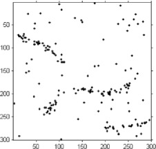
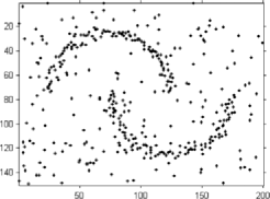
(a)	(b)
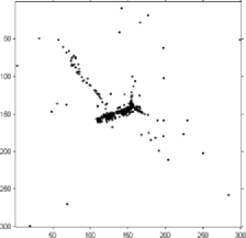
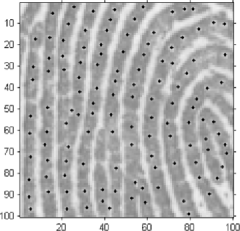
(c)	(d)

Figure 1: Four examples of point patterns clustered around latent curvilinear features with background noise. (a) Simulated point pattern. (b) Simulated point pattern described in Stanford and Raftery (2000). (c) Earthquake epicenters in the New Madrid region. Data is taken from CERI (Center for Earthquake Research and Information). (d) Pores along ridges of a portion of the fingerprint a002–05 from the NIST Special Database 30 [Watson (2001)].

The model introduced here describes families of nonintersecting curves via a field of orientations (a map $\upsilon_{\mathrm{FO}}\dvtx W\rightarrow[0,\pi)$ assigning an undirected orientation to each point in the window). The curves are produced as segments of streamlines integrating the field of orientations. We say that a curve integrates the field of orientations if the curve is continuously differentiable and of unit speed, and if its tangent agrees with the field of orientations at each point. The term streamline is used to describe a curve which integrates the field of orientations and has no end points in the interior of the window $W\setminus\partial{W}$.

We choose to use a variant on an empirical Bayes approach to estimate the field of orientations, since a fully Bayesian approach would involve infinite-dimensional distributions and be very computationally intensive. The empirical Bayes component consists of estimation of the field of orientations from the data via a tensor field as detailed in Section 4.1. In the following, a tensor field is represented by assignation of a symmetric nonnegative definite matrix to each point of the planar window. Tensor fields of this kind play an important role in diffusion tensor imaging [DTI, see Le Bihan et al. (2001)]. The field of orientations is constructed simply by calculating the orientations of the representative matrices’ principal eigenvectors; singularities in the field of orientations correspond to points where there is equality of the two eigenvectors.

We show how properties of the underlying distribution of fibres can be estimated using Monte Carlo techniques applied to the spatial point data. Our approach has the advantage that it can be used to quantify uncertainty on a range of parameters and does so effectively for different types of curvilinear structure. The use of a field of orientations to identify fibres leads to a strong performance on data such as that shown in Figure 1(d), where there is noticeable alignment of points perpendicular to the fibres.

1.1 Potential applications

Point patterns with a latent curvilinear structure arise in many different areas of study.

In seismology, epicenters of earthquakes are typically densely clustered around seismic faults. The earthquake data from the New Madrid region as shown in Figure 1(c) consists of one short dense cluster of points, one longer rather sparse cluster, both connected, and a relatively small number of “noise” points scattered over the window. The New Madrid earthquake data is considered in Stanford and Raftery’s (2000) approach to detecting curvilinear features.

In cosmology, galaxies appear to cluster along inter-connected filaments forming a three-dimensional web-like structure with large voids between the filaments. There is interest in identifying the nature of the filaments [see, e.g., Stoica, Martínez and Saar (2007)]. There is also evidence that these galaxies form surfaces or “walls” in some regions. This suggests the exciting challenge of extending our model to include two-dimensional surfaces in three-dimensional space.

A further application is that of sweat pore patterns on fingerprint ridges [see Figure 1(d)]. Sweat pores are tiny apertures along the ridges where the ducts of the sweat glands open. Robust inference of the ridge structure from the pore pattern has potential for aiding reconstruction of patchy fingerprints and may also allow for more efficient storage of fingerprints in very large databases. The underlying curve structure is a dense set of locally parallel curves along which pores are located, usually very close to the center of the ridges. The noise arises mostly from artifacts in the automatic extraction of pores from the image.

An issue with fingerprint pore data is that pores usually align across the ridges as well as along them. This can complicate the reconstruction of ridges, as the dominant orientation is less clear. We overcome this issue by constructing a smooth tensor field which extrapolates dominant orientation estimates over the regions of directional ambiguity.

1.2 Background

An existing method of estimating the curves in the underlying structure of a point process is Stanford and Raftery’s (2000) use of principal curves (a nonlinear generalization of the first principal component line). An EM-algorithm is used to optimize the model over a variety of choices of smoothness parameter and number of components. An optimal choice of smoothness and number of components is then selected using Bayes factors. This technique generally performs very well; however, it is sensitive to the initial clustering of the data and therefore has difficulties reconstructing fibres in some regions where fibres may be expected but signal points are absent [e.g., the fingerprint pore data—Figure 1(d)].

A piecewise linear “Candy model” (or “Bisous model” in three dimensions) is used by Stoica, Martínez and Saar (2007) to model filaments in galaxy data. They compare the empirical densities of galaxies within concentric cylinders and thus delineate these filaments. This approach is restricted to piecewise linear fibre models where the deviation of points from fibres follows a uniform distribution over a thin cylinder centered along the fibre. Sufficient statistics of the model for data with filamentary structure are then compared to sufficient statistics on structureless data sets; see Stoica et al. (2005) and Stoica, Martínez and Saar (2007, 2010).

Density estimates of the point pattern can be obtained using techniques such as kernel smoothing. Fibres can be directly estimated from this density; an example of this can be seen in Genovese et al. (2009) where steepest ascent paths along the density estimate are constructed and the density of these paths is analyzed.

A further approach discussed in Barrow, Bhavsar and Sonoda (1985) is based on construction of the minimal spanning tree of the set of points. In three dimensions this gives a useful insight into the overall characteristics of the filamentary structure.

The method presented in August and Zucker (2003) is based on a random curve model in which curvature is defined as a Brownian motion. The resulting model is used to enhance contours in the output of edge operators applied to digital images and thus to data in which signal points are dense along curvilinear structures.

The treatment advocated here is also based on the formulation of a general model for families of curves and the point patterns clustered around them. In contrast to August and Zucker (2003), curves are modeled as segments of streamlines integrating a smooth field of orientations which encourages interpolations over areas of missing data. The prior model for the orientation field is derived via an empirical Bayes step. Then birth–death MCMC is used to sample from the posterior distribution of the fibres. The model formulation itself uses the initial exploratory work of Su et al. (2008) [see also Su (2009)], which focused on the fingerprint pore data and described the use of tensor fields for estimating dominant orientations in spatial point data.

1.3 Problem definition

In particular, we are interested in modeling a random point process $\Pi$ viewed in a planar window $W\subset\mathbb{R}^{2}$; we write the observed part of the point process as $W\cap\Pi=\{y_{1},\ldots,y_{m}\}$ for some arbitrary ordering of points. The point process arises from a mixture of homogeneous background noise and an unknown number of point clusters, each clustered along a curve, henceforth called a fibre. Thus a fibre is a one-dimensional object, a smooth curved segment, embedded in a higher-dimensional space (the space containing the point process). Random sets of fibres or “fibre processes” are discussed in Stoyan, Kendall and Mecke (1995) and Illian et al. (2008).

Having specified an appropriate model, we must identify a suitable method of analysis of the posterior distribution of fibres given a data set of spatial point locations $\{y_{1},\ldots,y_{m}\}$ over the window $W$.

1.4 Plan of paper

The paper is laid out as follows. The following section gives an overview of the model proposed in this paper. Details of the underlying probability model are given in Section 3. The empirical Bayes method of estimating an appropriate field of orientations is outlined in Section 4. Section 5 presents a method of sampling from the posterior distribution of the fibres given the point pattern data using Monte Carlo methods. This is implemented for a number of examples in Section 6. In the final section we compare this model to other approaches, discuss some known issues of implementation and statistical analysis, and note possible directions in which this model might be extended.

2 Basic considerations

We use a Bayesian hierarchical model to describe the relationship between the points and the fibres.

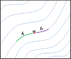
Figure 2: An orientation field is depicted as thin grey lines. A fibre $F(\omega,l_{1},l_{2})$ is defined as the curve segment that integrates the orientation field from reference point $\omega\in W$ in one direction to a distance $l_{1}$ and in the other direction to a distance $l_{2}$. Recall, a curve segment is said to integrate the orientation field if at any point of the segment its tangent agrees with the orientation field.

2.1 Points

A natural choice is to model the spatial point process as a mixed Poisson process or “Cox process” driven by a random fibre process. By this we mean that the points arise independently and are associated in some way with a random fibre—typically clustered around it. Such a point process is called a “fibre-process generated Cox process;” see Illian et al. (2008).

In our model we do associate points with particular fibres but we remove the Poissonian character of the distribution of points along fibres, replacing this by a renewal process based on Gamma distributions for interpoint distances. This allows us to model a tendency to regularity in the way in which points are distributed along a fibre but includes the Poissonian case with exponentially distributed interpoint distances.

2.2 Fibres

In contrast to previous work, in which curves are often constructed as splines fitted to the data, we define them as integral curves of a field of orientations. This means that at any point on a fibre, the tangent to the fibre agrees with the field of orientations at that point. Note that a field of orientations is equivalent to a vector field except that each point in the field is assigned a directionless orientation. An instance of a random field of orientations $\Upsilon_{\mathrm{FO}}$ is written as $\upsilon_{\mathrm{FO}}\dvtx W\rightarrow[0,\pi)$, where $[0,\pi)$ represents the space of planar directions (with $0$ and $\pi$ identified).

The simplest way to determine a fibre $F$ is to choose a reference point $\omega\in W$ on the fibre and specify the two arc lengths $l_{1},l_{2}\in{\mathbb{R}^{+}}$ of $F\setminus\{\omega\}$; see Figure 2. For a fixed field of orientations this will characterize a fibre, although the parametrization by reference point and length is evidently not unique. We model the fibres in terms of these parameters (the reference points, arc lengths and field of orientations). Note that an alternative construction can be based on random selection of a finite number of fibres generated by decomposing the streamlines according to Poisson point processes distributed along the streamlines; however, this construction introduces intriguing measure-theoretic issues which are out of place in the present treatment.

We note that taking the reference points to be uniformly distributed over the window $W$ will lead to a bias in the distribution of fibres in that the mean length of fibre per unit area is not constant across $W$. This issue has been considered and a solution involving an adjustment to the distribution of reference points has been identified. We have not applied the bias correction to our examples, as there is sufficient data to make the bias negligible.

The field of orientations is a useful intermediary in constructing fibres and, as such, is part of a useful decomposition of the construction problem. In practice, we seek to identify a suitable field of orientations by analysis of properties of the data.

2.3 Noise

Finally, we include background noise in the form of an independent homogeneous Poisson process superimposed onto the fibre-generated “signal” point process.

3 Probability model

A directed acyclic graph (or DAG) showing the conditional dependencies for the model is shown in Figure 3. A good introduction to directed acyclic graphs is given by Pearl (1988).

3.1 Fibres

Henceforth let $\mathbf{F}=\{F_{1},\ldots,F_{k}\}$ denote $k$ random fibres. As outlined earlier and illustrated in Figure 2, the fibre $F_{j}$ is determined by a reference point $\omega_{j}$ and arc lengths $l_{j,1},l_{j,2}$. It is also written $F_{j}=F_{j}(\omega_{j},l_{j},\nu_{\mathrm{FO}})$ [where $l_{j}=(l_{j,1},l_{j,2})$] to indicate that it is a deterministic function of $\omega_{j}$ and $l_{j}$ once $\nu_{\mathrm{FO}}$ is given. For the list of reference points we write $\bolds\omega=\{\omega_{1},\ldots,\omega_{k}\}$, and the arc length vectors are given by $\mathbf{l}=\{l_{1},\ldots,l_{k}\}$. We use $l_{j,T}=l_{j,1}+l_{j,2}$ as a shorthand for the total arc length of the $j$th fibre. Note that in general the orientation field $\upsilon_{\mathrm{FO}}$ may possess singularities, which would constrain the choice of the lengths $l_{j}=(l_{j,1},l_{j,2})$; however, this does not arise in our examples.

3.2 Signal points

Points from the observed pattern may be either signal or noise. Signal points are typically clustered around fibres. The model we use assigns an anchor point $p_{i}$ on some fibre to each data point $y_{i}$. The data point is then displaced from $p_{i}$ by an isotropic bivariate normal distribution [i.e., $y_{i}\sim\operatorname{MVN}(p_{i},\sigma_{\mathrm{disp}}^{2}\mathbf{I}_{2})$, where $\mathbf{I}_{2}$ is the $2\times 2$ identity matrix].

The fibre on which $p_{i}$ is located is determined by an auxiliary variable $X_{i}$, so $X_{i}=j$ if and only if $p_{i}\in F_{j}$. The $p_{i}$’s on the $j$th fibre are spaced such that the vector of arc-length distances between adjacent points is proportional to a Dirichlet distributed random variable. Setting an appropriate parameter for the Dirichlet distribution will encourage points to be either evenly spread, clustered along the fibre, or placed independently at random along the fibre.

The probability that point $y_{i}$ is allocated to the $j$th fibre ($X_{i}=j$) is proportional to the total length of fibre $F_{j}$. This ensures that the mean points per unit streamline remains approximately constant.

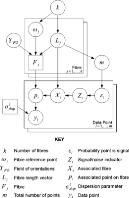
Figure 3: Directed acyclic graph (DAG) of model: arrows indicate conditional dependencies, elements in squares are deterministically calculated or constant, while those in circles are random variables. For simplicity we have not included reference to hyperparameters $\lambda$, $\kappa$, $\eta$, $\alpha_{\mathrm{signal}}$ and $\beta_{\mathrm{signal}}$.

3.3 Noise points

Noise is then added as a homogeneous Poisson process. This is included in the model by first allocating each point $y_{i}$ to noise or signal (stored in auxiliary variable $Z_{i}=1$ or $0$ for signal or noise, resp.). Point $y_{i}$ is allocated to signal independently of the allocations of all other points. The prior probability that $y_{i}$ is allocated to signal is given by $\varepsilon_{i}$. If the point is signal, then its location is distributed as outlined in the previous subsection. Otherwise, if the point is noise, it is distributed uniformly across the window $W$.

3.4 Total number of points

The total number of points $m$ is assumed to be Poisson distributed. The mean total number of points $\mu_{\mathrm{total}}$ is defined to be equal to some function of $\mu_{\mathrm{signal}}$, the mean number of signal points, and $\rho$, a parameter governing the number of noise points. For the sake of simplicity we set $\rho$ to be the prior assumption on the proportion of the total points that are noise points and define $\mu_{\mathrm{total}}=\mu_{\mathrm{signal}}/(1-\rho)$. The mean number of signal points $\mu_{\mathrm{signal}}$ is assumed to be proportional to the total sum of the fibre arc lengths. Hence, $m$ is assumed to be Poisson distributed with mean

$$\mu_{\mathrm{total}}=\Biggl{(}\sum_{j=1}^{k}(l_{j,T})\Biggr{)}\frac{\eta}{1-\rho},$$ (1)

where $\rho=\beta_{\mathrm{signal}}/({\alpha_{\mathrm{signal}}+\beta_{\mathrm{signal}}})$ is the prior estimate of the proportion of points that are signal and $\eta$ is a density parameter.

The assumption that the mean number of noise points is proportional to the mean total number of points (and the fibre length) is particularly well suited to the fingerprint example [see Section 6.3], where noise points arise as artifacts of the pore detection process along the fingerprint ridges. Implementation of alternative relationships between the mean number of signal and noise points would be a straightforward matter.

3.5 Priors

In the examples given in the next Section 6 we use the following priors:

$$P(\mathbf{l}|k,\lambda) = \prod_{j=1}^{k}P({l_{j,1}}|\lambda)P({l_{j,2}}|\lambda)\qquad\mbox{where }{l_{j,\cdot}}\sim\operatorname{Exp}(1/\lambda),$$

$$P(\bolds\omega|k) = \prod_{j=1}^{k}P(\omega_{j})\qquad\mbox{where }\omega_{j}\sim\operatorname{Uniform}(W),$$

$$P(k|\kappa) \sim \operatorname{Poisson}(\kappa),$$

$$P(\bolds{\epsilon}|\alpha_{\mathrm{signal}},\beta_{\mathrm{signal}}) = \prod_{i=1}^{m}P(\epsilon_{i}|\alpha_{\mathrm{signal}},\beta_{\mathrm{signal}})$$ (2)

$$\eqntext{\mbox{where }\epsilon_{i}\sim\operatorname{Beta}(\alpha_{\mathrm{signal}},\beta_{\mathrm{signal}}).}$$

Here $m$ is the total number of points in $\{y_{1},\ldots,y_{m}\}$.

The above prior models are common, parsimonious choices that appear flexible enough for a range of applications including the examples considered in Section 6. However, if application-specific prior information suggests alternative prior models, then these can be accommodated in the presented framework.

3.6 Posterior

We are interested in the posterior distribution of fibres (and various other parameters) given a particular instance of the point process. This posterior is given by

$$\pi(\mathbf{F},\mathbf{l},\bolds\omega,k,\upsilon_{\mathrm{FO}},\bolds{\epsilon},\mathbf{Z},\mathbf{X},\mathbf{p})$$

$$\qquad=P(\mathbf{F},\mathbf{l},\bolds\omega,k,\upsilon_{\mathrm{FO}},\bolds{\epsilon},\mathbf{Z},\mathbf{X},\mathbf{p}|\mathbf{y})$$

$$\qquad\propto P(\mathbf{F},\mathbf{l},\bolds\omega,k,\upsilon_{\mathrm{FO}},\bolds{\epsilon},\mathbf{Z},\mathbf{X},\mathbf{p})$$

$$\qquad\quad{}\times L(\mathbf{F},\mathbf{l},\bolds\omega,k,\upsilon_{\mathrm{FO}},\bolds{\epsilon},\mathbf{Z},\mathbf{X},\mathbf{p}|\mathbf{y})$$

$$\qquad=P(\mathbf{l}|k)P(\bolds\omega|k)P(k)P(\upsilon_{\mathrm{FO}})P(\bolds{\epsilon})P(\mathbf{Z}|\bolds{\epsilon})$$

$$\qquad\quad{}\times P(\mathbf{X}|\mathbf{Z},\mathbf{l})P(\mathbf{p}|\mathbf{F},\mathbf{X})L(\mathbf{F},\mathbf{l},\bolds\omega,k,\upsilon_{\mathrm{FO}},\bolds{\epsilon},\mathbf{Z},\mathbf{X},\mathbf{p}|\mathbf{y}).$$

Here $P(\cdot)$ indicates a prior distribution. We omit $P(\mathbf{F}|\mathbf{l_{1}},\mathbf{l_{2}},\bolds\omega,\upsilon_{\mathrm{FO}})$, as it is deterministically calculated.

Section 5 describes how to sample from this posterior distribution using Markov chain Monte Carlo techniques.

3.7 Computational simplifications

Computer implementation makes it necessary to represent the field of orientations by a discrete structure. We adopt the simple approach of estimating the field of orientations at a dense regular grid of points over $W$. Integral curves are calculated stepwise by estimating the orientation at a point by its value at the nearest evaluated grid point and extending the curve a small distance in that direction. Note that the choice of direction (from the two available for each orientation) is made so that the angle between adjacent linear segments is greater than $\pi/2$.

Consequently, fibres are stored as piecewise-linear curves and further calculations are performed on these approximations. Of course, this discretization can be arbitrarily reduced (at a computational cost) to improve the accuracy of the approximation.

4 Construction of field of orientations

We must of course identify a method for calculating the field of orientations. It is computationally advantageous to generate a field of orientations which is likely to contain (be integrated by) fibres that fit the data well (produce a high likelihood). The most natural way to do this is to base the calculation of the field of orientations on the data, using an empirical Bayes technique. The use of empirical Bayes to find the prior for the field of orientations distribution means that aspects of the prior, or parameters of the prior, are estimated from the data.

An alternative approach would be to use a fully Bayesian model, where we would treat the field of orientations as an independent random variable $\Upsilon_{\mathrm{FO}}$. We would then need to identify its state space and a corresponding $\sigma$-algebra, transition kernel and prior on this state space. These could be derived from random field theory [see, e.g., Adler and Taylor (2007)], using an appropriate covariance function to maintain smoothness in the field of orientations, however, there are a number of issues with this approach. In practice, one may expect the task of sampling a random field of orientations to be computationally expensive, particularly if the covariance function does not have a simple form (as is likely in this model). Calculations relating to the conditional distribution of the field of orientations given the fibres are likely to lead to unfeasible computational complexity. A further issue is that this approach leads to a huge space of possible fibres, resulting in corresponding difficulties in ensuring this space is properly explored. Use of the information given in the data will help to limit this space to a more easily explorable restricted class of suitable fields of orientations.

Here we use the data to make local orientation estimates and smooth these to produce a field of orientations estimator. As we are specifically interested in orientation estimates arising from the signal data, we can choose to weight the contribution of each point to the field of orientations estimator by how likely it is to be noise or signal.

Estimation of a field of orientations given that $y_{1},\ldots,y_{m}$ are all signal points is outlined in the following section. Section 4.2 shows how to extend this to take account of the information given in the vector of probabilities that points are signal $(\varepsilon_{1},\varepsilon_{2},\ldots,\varepsilon_{m})$.

4.1 Estimation for all signal points

The mapping and tensor method described in Su et al. (2008) [and further discussed in Su (2009)] is applied to the point pattern to construct a tensor at each point. To this we apply a Gaussian kernel smoothing in the log-Euclidean metric to construct a tensor field. The tensor field is represented by an assignation to each point of a $2\times 2$ nonnegative definite matrix whose principal eigenvector indicates the dominant orientation at that point; the relative magnitude of the eigenvalues indicates the strength of the dominant orientation. The field of orientations assigns the orientation of this principal eigenvector to each respective point. If the principal eigenvector is not unique at a certain point (which is to say that the eigenvalues are equal there), then that indicates a singularity in the field of orientations.

Three-dimensional tensor fields of this kind are commonly used in diffusion tensor imaging (DTI) to understand brain pathologies such as multiple sclerosis, schizophrenia and strokes. DTI is used to analyze images of the brain collected from magnetic resonance imaging (MRI) machines. The MRI scan detects diffusion of water molecules in the brain and uses the data to infer the tissue structure that limits water flow. The three-dimensional diffusion tensor describes the orientation dependence of the diffusion. Roughly speaking, the eigenvalues indicate a measure of the proportion of water molecules flowing in the associated eigenvector direction. For more information on DTI see, for example, Le Bihan et al. (2001) and Li et al. (2007).

Let $y_{1},\ldots,y_{m}$ denote the spatial data points. A tensor is constructed at a point $y_{j}$ using a nonlinear transformation applied to the vectors $v^{i}=(v_{1}^{i},v_{2}^{i})=\overrightarrow{y_{j}y_{i}}$ for $i\neq j$ [Su et al. (2008), Su (2009)]. Specifically,

$$\tilde{v}^{i}=(\tilde{v}^{i}_{1},\tilde{v}^{i}_{2})=\exp\biggl{(}-\frac{((v_{1}^{i})^{2}+(v_{2}^{i})^{2})}{2\sigma_{\mathrm{FO}}^{2}}\biggr{)}\frac{(v_{1}^{i},v_{2}^{i})}{\sqrt{(v_{1}^{i})^{2}+(v_{2}^{i})^{2}}},$$ (4)

where $\sigma_{\mathrm{FO}}$ is a scaling parameter.

The tensor at $y_{j}$ is then represented by

$$T_{0}(y_{j})=\sum_{i\neq j}(\tilde{v}_{1}^{i},\tilde{v}_{2}^{i})^{\mathrm{T}}(\tilde{v}_{1}^{i},\tilde{v}_{2}^{i}).$$ (5)

The result of the above method is to produce a set of $2\times 2$ matrices located over a sparse set of locations. In order to create a field of orientations, we must then interpolate to get a tensor field. Thus, we use the orientation of the principal eigenvector, where defined, to construct a field of orientations.

Interpolation of tensors inevitably requires a notion of tensor metric. We elect to work in the log-Euclidean metric [see Arsigny et al. (2006)]. For an extended account of tensor metrics see Dryden, Koloydenko and Zhou (2009). Log-Euclidean calculations are simply Euclidean calculations on the tensor logarithms which are transformed back to tensor space by taking the exponential. The tensors arising in this study can all be represented by positive definite matrices. Tensor logarithms are therefore well defined as logarithms of these matrices. However, the matrix calculated in (5) will have a zero-eigenvalue if the points are collinear, and therefore not be positive definite. If all points are truly collinear, then our approach breaks down—and indeed the method is not intended for such noise-free data sets. The more common situation is that one vector $\tilde{v}^{i}$ dominates the tensor representation as calculated in (5) due to the relative distances between points. Typically this occurs if two points are close while other points are far from the pair. Due to rounding errors, the contribution of other points to the matrix becomes zero, and the two remaining points are collinear by definition. In order to avoid an error in the log-Euclidean calculation, if a tensor has at least one zero-eigenvalue, then it is replaced by the “uninformative” identity matrix, suggesting a lack of directional information. Thus, we take a conservative approach that excludes any potentially misleading directional information.

We calculate the interpolated tensor field $T_{h_{\mathrm{FO}}}(x)$ for $(x\in W)$ as a kernel smoothing procedure, using a Gaussian kernel $f$ with variance parameter $h_{\mathrm{FO}}^{2}$ in the log-Euclidean metric. Hence, when the smoothing parameter $h_{\mathrm{FO}}$ is positive, $h_{\mathrm{FO}}>0$,

$$T_{h_{\mathrm{FO}}}(x)=\exp\biggl{(}\frac{\sum_{y_{i}\in\{y_{1},\ldots,y_{m}\}}f(\operatorname{dist}(x,y_{i}))\log(T_{0}(y_{i}))}{\sum_{y_{i}\in\{y_{1},\ldots,y_{m}\}}f(\operatorname{dist}(x,y_{i}))}\biggr{)}.$$ (6)

The field of orientations $\upsilon_{FO}(y_{1},\ldots,y_{m};h_{\mathrm{FO}})(x)$ for $x\in W$ is then defined to be equal to $\tan^{-1}(v_{1}(x)/v_{2}(x))$, where $(v_{1}(x),v_{2}(x))$ is the principal eigenvector of the matrix representation of $T_{h_{\mathrm{FO}}}(x)$.

In most instances this procedure will give a good estimation of a suitable field of orientations for modeling the point process with integral fibres. The smoothing method has the drawback that it can create a bias around areas of high curvature (rapidly varying orientation) in the field of orientations. Potential solutions have been analyzed and found to perform well. The magnitude of the bias was found to be proportional to the smoothing parameter $h_{\mathrm{FO}}$, hence, these solutions typically involve compensating for $h_{\mathrm{FO}}$: we give two examples: [(B)]

We allow the smoothing parameter to vary over the window, such that lower values are used in areas of high point intensity. This ensures that less information is extrapolated to regions where there is already sufficient data, and therefore less bias occurs in those regions.

We consider two instances of the field of orientations with different values of smoothing parameter $h_{\mathrm{FO}}^{\prime}$ and $h_{\mathrm{FO}}^{\prime\prime}$; the unbiased estimate can be found by extrapolating back to estimate the field of orientations with $h_{\mathrm{FO}}=0$. We do not go into further detail here because doing so would distract from the main ideas in this paper, but we do notice a minor effect of this bias in the examples in Section 6. Details of these bias corrections can be found in Hill (2011).

4.2 Estimation using signal probabilities

We extend this field of orientations estimation to take account of the vector of probabilities that points are signal $(\varepsilon_{1},\varepsilon_{2},\ldots,\varepsilon_{m})$ by weighting the construction of the initial tensor and also weighting the contribution of each initial tensor to the kernel smoothing.

Specifically, the initial tensors are represented by

$$T_{0}(y_{j})=\sum_{i\neq j}(\tilde{v}_{1}^{i},\tilde{v}_{2}^{i})^{\mathrm{T}}(\tilde{v}_{1}^{i},\tilde{v}_{2}^{i})\epsilon_{i}$$ (7)

for each point $y_{j}$, and the tensor field becomes

$$T_{h_{\mathrm{FO}}}(x)=\exp\biggl{(}\frac{\sum_{y_{i}\in\{y_{1},\ldots,y_{m}\}}\epsilon_{i}f(\operatorname{dist}(x,y_{i}))\log(T_{0}(y_{i}))}{\sum_{y_{i}\in\{y_{1},\ldots,y_{m}\}}\epsilon_{i}f(\operatorname{dist}(x,y_{i}))}\biggr{)}.$$ (8)

This weighting allows points that are more likely to be signal points to have a greater effect on the field of orientations estimation. As $\varepsilon_{i}\rightarrow 0$ the effect of the point $y_{i}$ on the field of orientations tends to zero, whereas if $\varepsilon_{i}=1$ for all $i$ we would be performing the calculation described in Section 4.1.

5 Sampling from the posterior distribution

We seek to infer some characteristics of the fibre process when only the point pattern is known. Typical attributes of interest include the number of fibres, where they are located/orientated, which points arose from which fibre and which points arose from background noise.

Direct inference from the model is hindered by the complexity of its hierarchical structure. Hence, we choose to draw samples from the posterior distribution of the fibres and other variables using Markov chain Monte Carlo methods. Characteristics of interest can be estimated from these samples.

5.1 Hyperparameters

As a rough guideline, hyperparameters can be chosen as follows.

The prior mean number of fibres $\kappa$ and the prior mean length of fibres $\lambda$ can be estimated from any prior knowledge or expectations of the fibres. The deviation of points from fibres $\sigma_{\mathrm{disp}}^{2}$ can be estimated using prior knowledge of fibre widths and the approximation that 95% of points should lie within $2.45\sigma_{\mathrm{disp}}$ of the center of a fibre. The density of points per unit length of fibre $\eta$ can be similarly estimated.

Orientation field parameters $h_{\mathrm{FO}}$ and $\sigma_{\mathrm{FO}}$ should be chosen to ensure the orientation field is smooth. These can be estimated by evaluating the orientation fields for different selections of $h_{\mathrm{FO}}$, $\sigma_{\mathrm{FO}}$ and choosing from this set. If the proportion of noise points is approximately known, then the hyperparameters $\alpha_{\mathrm{Signal}}$ and $\beta_{\mathrm{Signal}}$ can be suitably estimated, however, we suggest choosing the parameters such that $\alpha_{\mathrm{Signal}},\beta_{\mathrm{Signal}}>1$ to ensure good mixing properties of the Markov chain Monte Carlo sampling algorithm. Otherwise the noise hyperparameters can be set equal to $1$, indicating no prior knowledge.

Alternatively, if little prior information is known about the nature of the latent curvilinear structure, then it would be feasible to extend the empirical Bayes step to include the estimation of further prior parameters.

5.2 Birth–death Monte Carlo

The starting point for our algorithm is a continuous time birth–death Markov chain Monte Carlo (BDMCMC) in which fibres are created and die at random times controlled by predetermined or calculated rates. This enables exploration of a wide range of models with different numbers of fibres, and is suited to this type of clustered data. See Møller and Waagepetersen (2004) for an introduction to spatial birth–death processes. For the sake of brevity we present in the following the key points of the algorithm. Further details can be found in Hill (2011).

Here we choose to fix the birth rate and calculate an appropriate death rate at each step to maintain detailed balance.

Following a birth or death we update the following auxiliary variables: $\mathbf{Z}$ to $\mathbf{Z}^{\prime}$, the indicators of the components (signal/noise) to which the points are associated; $\mathbf{X}$ to $\mathbf{X}^{\prime}$, the indicators of the fibres to which the signal points are associated; $\mathbf{p}$ to $\mathbf{p}^{\prime}$, the vector $(p_{1},\ldots,p_{m})$ where $p_{i}$ is the point on the fibre to which the data point $y_{i}$ is associated.

5.3 Births of fibres

Recall that the parameterization of fibres is described in Section 2.2. Birth events occur randomly at rate $\beta$. Upon the occurrence of a birth, the number of fibres is updated from $k$ to $k+1$, and a new fibre is introduced by sampling a reference point $\omega_{k+1}$ and lengths $l_{k+1,1},l_{k+1,2}$ from the prior distributions $P(\omega),P(l)$, respectively. The new fibre $F_{k+1}$ is then calculated by integrating the field of orientations according to these parameters, and the set of fibres $\mathbf{F}=F_{1},\ldots,F_{k}$ is updated to $\mathbf{F}^{\prime}=F_{1},\ldots,F_{k},F_{k+1}$. In order to ensure that the distribution of the lengths $l_{k+1,1},l_{k+1,2}$ is independent of the respective directions in which the field of orientations is integrated, we choose them to be independently and identically distributed.

Data points which are currently assigned to the noise component are reassigned to noise or signal with proposal probability dependent on the new fibre $Q_{\mathrm{birth}}(\mathbf{Z}\mapsto\mathbf{Z}^{\prime}|\mathbf{Z},\bolds\varepsilon,F_{k+1})$.

Finally, new values are proposed for all of $\mathbf{X},\mathbf{p}$ according to a proposal density $Q(\mathbf{X},\mathbf{p}\mapsto\mathbf{X}^{\prime},\mathbf{p}^{\prime})$. For simplicity, we choose not to sample from the full conditional distribution of $\mathbf{p}$ and $\mathbf{X}$, but rather from a density proportional to the likelihood $L(\mathbf{p},\mathbf{X}|\mathbf{y})$.

In full, the birth density of fibre $F_{k+1}$ including updates of auxiliary variables to $\mathbf{Z}^{\prime},\mathbf{X}^{\prime},\mathbf{p}^{\prime}$ is given by

$$b(F_{k+1},\omega_{k+1},l_{1,{k+1}},l_{2,{k+1}},\mathbf{Z}^{\prime},\mathbf{X}^{\prime},\mathbf{p}^{\prime})$$

$$\qquad=\beta P(\omega_{k+1})P(l_{1,{k+1}})P(l_{2,{k+1}})Q_{\mathrm{birth}}(\mathbf{Z}\mapsto\mathbf{Z}^{\prime}|\mathbf{Z},\bolds\epsilon,F_{k+1})$$ (9)

$$\qquad\quad{}\times Q(\mathbf{X},\mathbf{p}\mapsto\mathbf{X}^{\prime},\mathbf{p}^{\prime}).$$

5.4 Deaths of fibres

We must calculate the death rate $\delta_{j}$ for each fibre to ensure detailed balance holds. Following the death of fibre $F_{j}$, the variables $\mathbf{F},\bolds\omega$ and $\mathbf{l}$ are updated by omitting the $j$th term. Further, auxiliary variables $\mathbf{Z},\mathbf{X}$ and $\mathbf{p}$ are all updated. All points allocated to fibre $F_{j}$ are now allocated to noise. We call this trivial proposal density $Q_{\mathrm{death}}(\mathbf{Z}^{\prime}|\mathbf{Z},\mathbf{X},j)$. Again the final step is to propose new values for all of $\mathbf{X}$ and $\mathbf{p}$ according to proposal density $Q(\mathbf{X},\mathbf{p}\mapsto\mathbf{X}^{\prime},\mathbf{p}^{\prime})$.

Hence, the death rate that satisfies detailed balance for the $j$th fibre is given by

$$\delta_{j} = \frac{P(\mathbf{l_{1}}\setminus l_{1,j},\mathbf{l_{2}}\setminus l_{2,j}|k-1)}{P(\mathbf{L_{1}},\mathbf{L_{2}}|k)}\frac{P(\bolds\omega\setminus\omega_{j}|k-1)}{P(\bolds\omega|k)}\frac{P(k-1)}{P(k)}$$

$${}\times\frac{b(F_{j},\omega_{j},l_{1,j},l_{2,j},\mathbf{Z}^{\prime},\mathbf{X}^{\prime},\mathbf{p}^{\prime})}{Q_{\mathrm{death}}(\mathbf{Z}^{\prime}|\mathbf{Z},\mathbf{X},j)Q(\mathbf{X},\mathbf{p}\mapsto\mathbf{X}^{\prime},\mathbf{p}^{\prime})}$$

$$= \frac{P(k-1)}{P(k)}\frac{\beta Q_{\mathrm{birth}}(\mathbf{Z}^{\prime}\mapsto\mathbf{Z}|\bolds\epsilon,F_{j})Q(\mathbf{X}^{\prime},\mathbf{p}^{\prime}\mapsto\mathbf{X},\mathbf{p})}{Q_{\mathrm{death}}(\mathbf{Z}^{\prime}|\mathbf{Z},\mathbf{X},j)Q(\mathbf{X},\mathbf{p}\mapsto\mathbf{X}^{\prime},\mathbf{p}^{\prime})}.$$

5.5 Additional moves

It can be desirable to add extra moves to the BDMCMC process to improve mixing. Some possible moves which were all utilized in the examples in Section 6 include the following:

• moving a fibre by a small amount (by perturbing the reference point),

• resampling the lengths of a fibre (while keeping the reference point fixed).

Each of these events occur at some predefined rate, whence they are proposed and either accepted or rejected according to the Metropolis Hastings probability.

We may also wish to update other model variables, giving more flexibility and improving the algorithm’s exploration of the sample space. The additional variable updates used in the examples in Section 6 include the following:

• proposing new signal-noise allocations of the data ($\mathbf{Z}$),

• proposing new signal probabilities ($\bolds\varepsilon$) according to nondegenerate Beta distributions whose parameters depend on the current signal- noise allocations $\mathbf{Z}$. This move leads to an update in the prior for the field of orientations due to the empirical Bayes step, hence, all fibres are resampled.

Details of all moves can be found in Hill (2011).

Hyperprior parameters, such as the constant of proportionality $\eta$ in the prior for the Poisson-distributed number of points or $\sigma_{\mathrm{disp}}$ governing the deviation of points from fibres, may also be updated. We have chosen not to update any hyperprior parameters to reduce complexity of the model.

5.6 Convergence and output analysis

First recall that the signal probabilities $\bolds\varepsilon$ are updated according to nonsingular Beta distributions. Hence, the underlying tensor field as defined in (8) will not become degenerate even when $\mathbf{Z}$ allocates all points to noise.

Consider the set $A$ of states in which the fibre configuration is empty and all points are allocated to noise. In the following discussion we exclude any degenerate states of equilibrium probability zero. Inspection of the algorithm shows that the set $A$ can be reached from any nondegenerate state in finite time and so the birth–death process is $\phi$-irreducible. Recurrence can be deduced by noting that the set $A$ is visited infinitely often; see Kaspi and Mandelbaum (1994).

We motivate a heuristic lower bound on a suitable burn-in time by considering aspects of the prior derived after inspection of the data (e.g., $\sigma_{\mathrm{disp}},\lambda,\kappa$—see Section 5.1), and estimating the number of fibre births that must occur before a fibre has been created around each potential fibre cluster. We approximate the lower bound by considering the number of fibre births required for this to happen around the smallest suitable cluster of points.

A lower bound on half the length of the shortest suitable cluster is derived from the $10\%$ quantile of an exponentially distributed random variable of rate $\kappa/\lambda$. Then the probability that a point chosen at random from $W$ lies in a region corresponding to an actual fibre of this length (up to $2\sigma_{\mathrm{disp}}$ from the fibre) is approximated by

$$\frac{8\lambda\log(10/9)\sigma_{\mathrm{disp}}}{\kappa|W|}.$$ (11)

It follows that, with probability $0.99$, a fibre will be proposed in the region corresponding to the shortest fibre within the first

$$\frac{\log(0.01)}{\log(1-{8\lambda\log(10/9)\sigma_{\mathrm{disp}}}/({\kappa|W|}))}$$ (12)

births. Hence, we choose a burn-in time of

$$T_{\mathrm{burn}}=\max\biggl{\{}1500,\frac{\log(0.01)}{\beta\log(1-{8\lambda\log(10/9)\sigma_{\mathrm{disp}}}/({\kappa|W|}))}\biggr{\}},$$ (13)

taking 1500 as a lower bound to ensure the burn-in time remains substantial.

Convergence was assessed by considering variables such as the number of fibres $k$ or the number of noise points and using Geweke’s spectral density diagnostic; see Brooks and Roberts (1998). Convergence of a sequence of $n$ samples is rejected if the mean value of the variable in the first $n/10$ samples is not sufficiently similar to the mean value over the last $n/2$ samples.

We also tested convergence by assessing whether the mean sum of the death rates is approximately equal to the birth rate $\beta$. Consider $\delta_{\mathrm{total}}^{k}t^{k}$ where $\delta_{\mathrm{total}}^{k}$ is the sum of the death rates of fibres after the $k$th event (e.g., birth, death, etc.) and $t^{k}$ is the length of algorithmic time before the next event. If the MCMC has reached stationarity, then

$$Z_{m}=\frac{\sum_{k=1}^{m}\delta_{\mathrm{total}}^{k}t^{k}-m\beta/(2\beta+r_{\mathrm{add}})}{\sigma_{\delta_{\mathrm{total}}t}\sqrt{m}}\stackrel{{\scriptstyle D}}{{\rightarrow}}N(0,1),$$ (14)

where $\sigma_{\delta_{\mathrm{total}}t}$ is an estimate of the standard deviation of $\delta_{\mathrm{total}}^{k}t^{k}$, $\beta$ is the birth rate of fibres, and $r_{\mathrm{add}}$ is the sum of the rates of any additional moves implemented (as suggested in Section 5.5). We used this result to test the convergence of $1/m\sum_{k=1}^{m}\delta_{\mathrm{total}}^{k}t^{k}$ to $\beta/(2\beta+r_{\mathrm{add}})$.

Bearing in mind the complexities of the underlying model, output analysis showed no evidence for a lack of convergence.

Outputs of various variables are recorded at random times at some constant rate. The rate of this sampling (effectively the reciprocal of the thinning of the Monte Carlo process) is chosen such that there is a low probability that any of the fibres remain unchanged between samples. The inclusion of the extra moves designed to improve mixing also helps to decrease the thinning required. The thinning is chosen approximately proportional to the number of fibres (estimated based on aspects of priors derived from inspection of the data).

6 Simulation studies and applications

The implemented algorithm runs on a continuous time scale. Events occur at a determined rate, either fixed or calculated to ensure that detailed balance holds. The units for the rate of an event are “per unit of algorithm time.” The BDMCMC is then allowed to run for a large number of time units and samples are taken at random times (at some fixed rate). Of course, the relationship of algorithm time to actual processing time depends on hardware and implementation details. Hardware details are described below.

In each of the following examples, the birth rate and the rate of other moves (moving a fibre, adjusting lengths of a fibre, proposing a split or a join, variable updates) were all unit rate. The only exceptions were the signal probability ($\bolds\varepsilon$) updates which were proposed at a rate of $0.1$ per unit of time, and the recording of output variables at random times whose rate varied for different data sets.

We evaluate the field of orientations over a square grid of points, each one unit length from its four nearest neighbors. The total size of this grid is given by the dimensions of the window $W$.

All three examples were run on the cluster owned by the Statistics Department in the University of Warwick using a Dell PowerEdge 1950 server with a 3.16 GHz Intel Xeon Harpertown (X5460) processor and 16 GB fully-buffered RAM. The algorithm was implemented in Octave version 3.2.4. The total run-times on the cluster ranged from 34.7 hours for the fingerprint pore data (32,300 units of algorithm time) to 61.3 hours for the earthquake data set (30,000 units of algorithm time). Due to the limitations of the current version of Octave, the benefits of a parallel implementation have not yet been explored.

Analysis has been performed on all four of the data sets shown in Figure 1. However, for the sake of brevity, we omit discussion of results for the first simulated point pattern [Figure 1(a)] from this paper.

6.1 Simulated example

Figure 4(a) shows the simulated data set used in Stanford and Raftery (2000). We include it here to facilitate comparison with the methods proposed by Stanford and Raftery. The data consists of 200 signal points and 200 noise points over a $200\times 150$ window, and is based on a family of two fibres each of length 157.

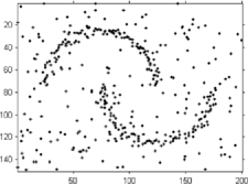
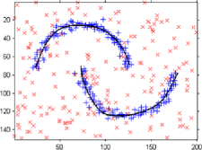
(a)	(b)
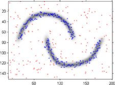
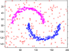
(c)	(d)

Figure 4: Simulated example from Stanford and Raftery (2000). (a) Simulated data. (b) A random sample from the BDMCMC output. Fibres are represented by curves, pluses indicate points allocated to signal and crosses indicate points allocated to noise in this sample. (c) Estimate of the density of signal points found by smoothing a series of samples of fibres (darker areas indicate higher densities). Pluses indicate points allocated to signal and crosses indicate points allocated to noise in at least $50\%$ of samples. The size of points representing the data has been reduced to enhance the clarity of the density estimate. (d) Estimate of the clustering of the signal points—different symbols indicate different clusters, crosses indicate noise. Estimated by considering how often pairs of points are associated with the same fibre across a number of samples.

Table 1: Results for Stanford and Raftery’s simulated example: first sub-table gives posterior probabilities on the number of fibres, while the second gives posterior means and 50% and 95% HPD (highest posterior density) intervals for a selection of properties of the posterior distribution conditional on the number of fibres. The simulated data consists of 200 signal points and 200 noise points over a $200\times 150$ window, and is based on a family of two fibres each of length 157. The dispersion parameter $\sigma_{\mathrm{disp}}$ is set to 3 and the prior mean probability that a point is noise is $0.5$. Posterior probabilities only given if nonzero to rounding error

	Posterior probabilities for number of fibres
Number of fibres		$2$	3.00	4.00
Posterior probability		$0.73$	0.23	0.04
	Other properties conditioned on the number of fibres
	Number of	Posterior	50% HPD	95% HPD
	fibres	mean	interval	interval
Number of noise points	2	$181.85$	$[176,193]$	$[156,205]$
	3	$180.81$	$[179,197]$	$[149,201]$
	4	$178.78$	$[167,184]$	$[155,197]$
95th percentile of the distances	2	$8.16$	$[7.17,8.32]$	$[6.64,9.66]$
from signal points to fibres	3	$8.06$	$[7.28,8.27]$	$[6.61,9.53]$
	4	$7.95$	$[7.20,7.91]$	$[6.75,9.50]$
Total length of fibres	2	$317.68$	$[319,325]$	$[301,325]$
	3	$319.60$	$[315,322]$	$[300,342]$
	4	$320.10$	$[325,303]$	$[303,325]$

The birth–death MCMC was run for 60,000 units of algorithm time, the first 30,000 of which were discarded. Samples were taken at a rate of $0.033$ per unit of time. The initial state was a randomly sampled set of $\kappa=2$ fibres. Other hyperparameters were chosen as follows: dispersion parameter $\sigma_{\mathrm{disp}}=3$; signal probability hyperparameters $\alpha_{\mathrm{signal}}=1$ and $\beta_{\mathrm{signal}}=1$; density parameter $\eta=0.64$; mean half-fibre length $\lambda=78.5$; and the Dirichlet parameter $\alpha_{\mathrm{Dir}}=1.5$.

Figure 4(b)–(d) shows that our model fits the data very well, albeit with a slight extrapolation of fibres beyond the curves used to generate the data set. The two fibres in the sample in Figure 4(b) compare favorably with the principal curves fitted in Stanford and Raftery (2000).

Table 1 gives the posterior probabilities of the number of fibres and the means and highest posterior density intervals of a variety of properties conditional on the number of fibres. The number of fibres is simply a count of the fibres present in each sample; in this example we expect it to be around 2. The number of points assigned to the noise component will typically be closely correlated with the number of fibres. With more fibres comes a greater chance of there being a fibre close to a given point and hence a greater chance that it is a signal point. We take the 95th percentile of the distances of signal points from their associated points on fibres for each sample. This summarizes the dispersion of points from the fibres. It is comparable to $2.45\sigma_{\mathrm{disp}}$, where $\sigma_{\mathrm{disp}}$ is the dispersion parameter (set to $3$ in this example). The constant $2.45$ arises as the 95th percentile of the Euclidean distance from the origin to a bivariate standard-normal distributed random variable. The curvature bias in the field of orientations results in a mild bias on the 95th percentile of distances from signal points to anchor points.

In this example, less points are associated to noise than were simulated as noise points in the data generation. This is partly due to the high intensity of noise points, and also explained by a slight bias in the length of the fibres. The posterior statistics on the lengths of the fibres suggest that the extension of fibres beyond their known length (of $157$) is supported by the high intensity of noise points. This extrapolation is sometimes beneficial, particularly for fibre reconstruction in areas of missing data. Here the extrapolation is less desirable, as it suggests there is evidence for fibres in the background noise.

The extrapolation of fibres into less dense regions of points can be reduced by choosing a higher Dirichlet parameter $\alpha_{\mathrm{Dir}}$ for the distribution of anchor points along the fibres. This decreases the posterior density of fibres lying through point clusters of nonconstant intensity. The drawback of increasing $\alpha_{\mathrm{Dir}}$ is that a large value of $\alpha_{\mathrm{Dir}}$ leads to a multimodal anchor point distribution with most of the probability mass concentrated at the modes. As the proposal of a birth/change of a fibre does not take account of the shape of anchor point distribution, the proposal of a state with low posterior density is more likely for larger $\alpha_{\mathrm{Dir}}$.

6.2 Application: Earthquakes on the new Madrid fault line

The epicenters of earthquakes along seismic faults are a good example of point data clustered around a system of fibres with additional background noise. Here the fibres are the unknown fault lines. Stanford and Raftery (2000) consider the structure of the data set of earthquakes around the New Madrid fault line in central USA. We use data on earthquakes in the New Madrid region between 1st Jan 2006 and 3rd Aug 2008 (inclusive) taken from the CERI (Center for Earthquake Research and Information) found at http://www.ceri. memphis.edu/seismic/catalogs/cat_nm.html.

The birth–death MCMC was run for 40,000 units of algorithm time, the first 10,000 of which were discarded. Samples were taken at a rate of $0.0167$ per unit of time. The initial state was a randomly sampled set of $\kappa=4$ fibres. Other hyperparameters were chosen as follows: dispersion parameter $\sigma_{\mathrm{disp}}=2$; signal probability hyperparameters $\alpha_{\mathrm{signal}}=4$ and $\beta_{\mathrm{signal}}=1$; density parameter $\eta=1.06$; mean half-fibre length $\lambda=30$; and the Dirichlet parameter $\alpha_{\mathrm{Dir}}=1.5$.

Table 2 gives some numerical properties of the posterior distribution of fibres.

Table 2: Results for earthquake data: first sub-table gives posterior probabilities on the number of fibres, while the second gives posterior means and 50% and 95% HPD (highest posterior density) intervals for a selection of properties of the posterior distribution conditional on the number of fibres. The data are all the recorded earthquakes in the New Madrid region between 1st Jan 2006 and 3rd Aug 2008; the data were acquired from the CERI (Center for Earthquake Research and Information) found at http://www.ceri.memphis.edu/ seismic/catalogs/cat_nm.html. In total there are 317 points in a $300\times 300$ window, the dispersion parameter $\sigma_{\mathrm{disp}}$ is set to 2 and the prior mean probability that a point is noise is $0.2$. Posterior probabilities only given if nonzero to rounding error

	Posterior probabilities for number of fibres
Number of fibres		$6$	7.00	8.00
Posterior probability		$0.56$	0.36	0.07
	Other properties conditioned on the number of fibres
	Number of	Posterior	50% HPD	95% HPD
	fibres	mean	interval	interval
Number of noise points	6	$42.99$	$[41,44]$	$[38,48]$
	7	$40.65$	$[38,41]$	$[36,45]$
	8	$42.06$	$[42,44]$	$[35,45]$
95th percentile of the distances	6	$5.25$	$[4.94,5.19]$	$[4.96,5.60]$
from signal points to fibres	7	$5.29$	$[5.12,5.40]$	$[4.85,5.89]$
	8	$5.17$	$[4.94,5.22]$	$[4.74,5.65]$
Total length of fibres	6	$257.24$	$[247,257]$	$[246,269]$
	7	$257.43$	$[257,262]$	$[249,264]$
	8	$252.89$	$[250,252]$	$[248,265]$

(a)	(b)
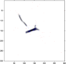
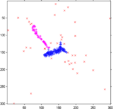
(c)	(d)

Figure 5: New Madrid fault earthquake data. (a) Earthquake data. (b) A random sample from the BDMCMC output. Fibres are represented by curves, pluses indicate points allocated to signal and crosses indicate points allocated to noise in this sample. (c) Estimate of the density of signal points found by smoothing a series of samples of fibres (darker areas indicate higher densities). Pluses indicate points allocated to signal in at least $50\%$ of samples. The size of points representing the data has been reduced to enhance the clarity of the density estimate. (d) Estimate of the clustering of the signal points—different symbols indicate different clusters, crosses indicate noise. Estimated by considering how often pairs of points are associated with the same fibre across a number of samples.

Our method has the advantage over Stanford and Raftery (2000), in that it does not try to over-fit the fibres where there is less data. Rather it uses information from surrounding data to extrapolate fibres as required. One limitation of our model is that every fibre is assumed to share a number of properties. In particular, the displacement of points from fibres (effectively the width of influence of a fibre) and the intensity of signal points per unit length of fibre are assumed to be constant, independent of the fibre. These assumptions are not reasonable for this data as the “thickness” and density of points varies considerably. This is apparent in Figure 5(b) where the central dense cluster is described by multiple parallel fibres. The dispersion parameter $\sigma_{\mathrm{disp}}$ was chosen by considering the apparent “width” of the longer thinner fibre, hence, points around the shorter, wider fibre effectively increase the 95th percentile of the point to fibre distances, as given in Table 2. To overcome this issue, one could extend the model to allow different hyperparameters for each fibre.

While multiple fibres in the central cluster is a common feature in samples from this BDMCMC, Figure 5(d) indicates that the agglomerative clustering algorithm identifies the points as arising from the same cluster.

Interestingly, the total length of fibres does not appear to be positively correlated to the number of fibres, suggesting that the additional fibres arise from splitting a fibre into multiple parts while preserving the total fibre length.

6.3 Application: Fingerprint data

The second application we consider is that of pores lying along ridge lines in fingerprints. Fingerprint pore data is considered in some depth in Su et al. (2008) and Su (2009).

We used a portion of the data set extracted from fingerprint a002–05 from the NIST (National Institute of Standards and Technology) Special Database 30 [Watson (2001)].

(a)	(b)
(c)	(d)

Figure 6: Pores from portion of fingerprint a002–05 from the NIST Special Database 30 [Watson (2001)]. (a) Pore data. (b) A random sample from the BDMCMC output. Fibres are represented by curves, pluses indicate points allocated to signal and crosses indicate points allocated to noise in this sample. (c) Estimate of the density of signal points found by smoothing a series of samples of fibres (darker areas indicate higher densities). The size of points representing the data has been reduced to enhance the clarity of the density estimate. (d) Estimate of the clustering of the signal points—different symbols indicate different clusters, crosses indicate noise. Estimated by considering how often pairs of points are associated with the same fibre across a number of samples.

The birth–death MCMC was run for 40,000 units of algorithm time, the first 8000 of which were discarded. Samples were taken at a rate of $0.007$ per unit of time. The initial state was a randomly sampled set of $\kappa=10$ fibres.

The fingerprint pore data will typically cause breakdown of nearest neighbor clustering methods. This is because, while the fibrous structure of the point pattern is clear when viewing the global picture, it is not so apparent on a small scale. This phenomena is partly due to the apparent inter-ridge alignment of points [from left to right in Figure 6(a)]. By way of contrast, our field of orientations model takes any information available on a small scale and uses it across the window, thanks to the smoothing step in the field of orientations.

As Figure 6 shows, our model succeeds in fitting many of the fibres (or fingerprint ridges) to the pore data. Figure 6(c) indicates areas of doubt in the fibre locations where the shading is lighter near the edges of the window, showing that fibre samples were more dispersed.

This data set is an ideal candidate for reconstruction of missing data. We work under the assumptions that pores lie at fairly regularly intervals along ridges, but some are not identified during the pore extraction process. Our method uses information from nearby ridges to complete fibres where data is missing. In this example this is particularly evident in the region below the center of the window. Knowledge of the posterior distribution of fibres could lead to a “filling in the gaps” approach to reconstructing the missing pore data.

Table 3 gives some numerical properties of the posterior distribution of fibres.

Table 3: Fingerprint Pore Data Set: Posterior means and 50% and 95% credible intervals of a selection of properties of the posterior distribution conditional on the number of fibres. The data was extracted from a portion of fingerprint a002–05 from the NIST (National Institute of Standards and Technology) Special Database 30 [Watson (2001)]. It consists of 123 points on a $100\times 100$ window. A dispersion parameter of $\sigma_{\mathrm{disp}}=1.5$ is used, and the mean prior probability a point is noise is $0.091$. Posterior probabilities only given if nonzero to rounding error

	Posterior probabilities for number of fibres
Number of fibres	$13$	$14$	$15$	$16$	$17$	$18$	$19$	$20$
Posterior probability	$0.03$	$0.11$	$0.17$	$0.17$	$0.25$	$0.11$	$0.09$	$0.05$

	Other properties conditioned on the number of fibres
	Number of	Posterior	50% HPD	95% HPD
	fibres $\bolds{k}$	mean	interval	interval
Number of noise points	14	$14.45$	$[14,16]$	$[9,18]$
	15	$15.71$	$[12,15]$	$[12,21]$
	16	$15.00$	$[12,17]$	$[8,21]$
	17	$18.86$	$[16,19]$	$[16,23]$
	18	$16.08$	$[15,18]$	$[10,25]$
95th percentile	14	$3.76$	$[3.74,3.82]$	$[3.25,4.22]$
of the distances	15	$3.68$	$[3.52,3.69]$	$[3.32,4.77]$
from signal points	16	$3.56$	$[2.34,3.52]$	$[3.34,3.89]$
to fibres	17	$3.58$	$[3.38,3.64]$	$[3.23,3.95]$
	18	$3.67$	$[3.44,3.75]$	$[3.24,4.38]$
Total length of fibres	14	$862.18$	$[861,883]$	$[785,964]$
	15	$882.38$	$[872,933]$	$[818,966]$
	16	$864.75$	$[836,886]$	$[784,927]$
	17	$814.43$	$[788,804]$	$[788,878]$
	18	$861.76$	$[821,876]$	$[761,941]$

7 Discussion

In this paper we have identified a new model for fibre processes and for point processes generated from a fibre process. We have shown how Monte Carlo methods can be used to sample from the posterior distribution of a fibre process that is instrumental in generating a point process.

Many different data sets of this type arise in nature. We investigated earthquakes that cluster around fault lines and pores in fingerprints that are situated along the fingerprint ridges. Other data can be found in catalogues of galaxies in the visible universe. Galaxies are known to align themselves along “cosmic” filaments which, in turn, connect to form a web-like structure. Understanding these fibres and identifying where they lie is of great interest to cosmologists; see, for example, Martínez and Saar (2002) for a statistical overview of some current ideas and also Stoica, Martínez and Saar (2007) for a different approach to modeling the filament structure. Other data sets for which this model may be suitable include the locations of land mines, often placed in straight lines. Identifying these lines may aid in the discovery of currently undetected mines. Similar methods of detecting structure in noisy pictures are a prominent area of research in image recognition.

This process can be used to fit nonparametric curves to point patterns with just two limitations on the nature of the curves. The limitations are that the curves must not intersect, and that they must be “sufficiently” smooth (i.e., there must be no acute angles in the discretization of the fibres). The smoothness property is desirable to identify smooth curves rather than complex structures. The nonintersection property may be less desirable but, at some computational cost, the model could be generalized to allow each fibre to integrate a different field of orientations.

We do not make use of a deterministic algorithm (such as the EM-algorithm) to fit the fibres, and our approach is not highly sensitive to the choice of starting parameters. Therefore, it can be used to provide interval estimates for various parameters. One of the most sensitive parameters fixed in the algorithm is $\sigma_{\mathrm{disp}}^{2}$ which governs the deviation of points from the fibres. If chosen too large, the result will be too few fibres with a sizeable error in their locations. If chosen too small, fibre clusters may be split into multiple parallel smaller clusters. Our experience is that the algorithm is reasonably robust to changes in other parameters.

One strength of our model is that it fits the noise-signal and cluster allocations implicitly, in contrast to other cases where the clustering may need to be predetermined. The advantage is that we can produce reliability estimates for these clustering and noise allocations and explore more potential clustering configurations, and hence more fibre structures.

A limitation of our model arises from the constraints on the similarity of fibres. Fibres are assumed to be of the same width (the displacement of points from the fibres is independent of the fibre), and have the same mean points per unit fibre length. These are not always reasonable assumptions, as is evidenced by the earthquake data set. We could extend the model to allow parameters $\sigma_{\mathrm{disp}}^{2}$ and $\eta$ to take different values for each fibre in order to eliminate this issue. A further extension would be to include isotropic clusters of points which do not fit well to the “fibre” model.

The complexity of the model, considering the infinite dimensionality of the field of orientations, raises the question of whether or not the Markov chain adequately explores the sample space. Our examples indicate that, while the sample space of fields of orientations is not explored particularly well, the space of fibre configurations is well explored and the field of orientations varies enough to explore a wide space of fibre configurations. However, as the density of fibres increases, so the MCMC algorithm requires longer runtime in order to overcome these issues.

Note that while our model performs as well as other available techniques on the basic data sets, it demonstrates significantly better performance on the fingerprint data where a large number of dense fibre clusters account for most of the data.

It is necessary to bear in mind the ramifications of edge effects in the model and subsequently the MCMC algorithm. As we are sampling from a bounded subset $W\subseteq\mathbb{R}^{2}$, the omission of potential points just outside $W$ induces a bias on distance-related measures. The field of orientations will have a bias at the edge favoring orientations parallel to the sides of a rectangular window $W$. Fibres are created by sampling a random reference point from the field and integrating the field of orientations from that point. However, the reference point cannot be sampled from outside $W$, and fibres that extend past the boundary of $W$ are typically terminated on the border as no field of orientations is available past that point. Also, the model for the displacement of points from fibres does not account for edge effects. Most of these algorithmic biases would be significantly decreased by creating a border around $W$ and completing the analysis over the whole area. However, this would come at an additional computational cost.

We have commented in passing on the phenomenon of curvature bias and its effects on the estimation of parameters, and we note this as a fruitful area for future research. Further research possibilities include the fitting of two-dimensional surfaces in 3 dimensions. Then new geometric issues need to be taken into account; for example, it is not the case that a generic field of tangent planes can be developed into a fibration by surfaces. It is hoped to investigate this problem in further work.

References

- Adler and Taylor (2007) {bbook}[author] \bauthor\bsnmAdler, \bfnmR. J.\binitsR. J. and \bauthor\bsnmTaylor, \bfnmJ. E.\binitsJ. E. (\byear2007). \btitleRandom Fields and Geometry. \bpublisherSpringer, \baddressNew York. \bidmr=2319516 \bptokimsref \endbibitem
- Arsigny et al. (2006) {barticle}[pbm] \bauthor\bsnmArsigny, \bfnmVincent\binitsV., \bauthor\bsnmFillard, \bfnmPierre\binitsP., \bauthor\bsnmPennec, \bfnmXavier\binitsX. and \bauthor\bsnmAyache, \bfnmNicholas\binitsN. (\byear2006). \btitleLog-Euclidean metrics for fast and simple calculus on diffusion tensors. \bjournalMagn. Reson. Med. \bvolume56 \bpages411–421. \biddoi=10.1002/mrm.20965, issn=0740-3194, pmid=16788917 \bptokimsref \endbibitem
- August and Zucker (2003) {barticle}[author] \bauthor\bsnmAugust, \bfnmJonas\binitsJ. and \bauthor\bsnmZucker, \bfnmSteven W.\binitsS. W. (\byear2003). \btitleSketches with curvature: The curve indicator random field and Markov processes. \bjournalIEEE Trans. Pattern Anal. Mach. Intell. \bvolume25 \bpages387–400. \bptokimsref \endbibitem
- Barrow, Bhavsar and Sonoda (1985) {barticle}[author] \bauthor\bsnmBarrow, \bfnmJ. D.\binitsJ. D., \bauthor\bsnmBhavsar, \bfnmS. P.\binitsS. P. and \bauthor\bsnmSonoda, \bfnmD. H.\binitsD. H. (\byear1985). \btitleMinimal spanning trees, filaments and galaxy clustering. \bjournalRoyal Astronomical Society, Monthly Notices \bvolume216 \bpages17–35. \bptokimsref \endbibitem
- Brooks and Roberts (1998) {barticle}[author] \bauthor\bsnmBrooks, \bfnmS. P.\binitsS. P. and \bauthor\bsnmRoberts, \bfnmG. O.\binitsG. O. (\byear1998). \btitleConvergence assessment techniques for Markov chain Monte Carlo. \bjournalStatist. Comput. \bvolume8 \bpages319–335. \bptokimsref \endbibitem
- Dryden, Koloydenko and Zhou (2009) {barticle}[author] \bauthor\bsnmDryden, \bfnmI. L.\binitsI. L., \bauthor\bsnmKoloydenko, \bfnmA.\binitsA. and \bauthor\bsnmZhou, \bfnmD\binitsD. (\byear2009). \btitleNon-Euclidean statistics for covariance matrices, with applications to diffusion tensor imaging. \bjournalAnn. Appl. Stat. \bvolume3 \bpages1102–1123. \biddoi=10.1214/09-AOAS249, issn=1932-6157, mr=2750388 \bptokimsref \endbibitem
- Genovese et al. (2009) {barticle}[author] \bauthor\bsnmGenovese, \bfnmC. R.\binitsC. R., \bauthor\bsnmPerone-Pacifico, \bfnmM.\binitsM., \bauthor\bsnmVerdinelli, \bfnmI.\binitsI. and \bauthor\bsnmWasserman, \bfnmL.\binitsL. (\byear2009). \btitleOn the path density of a gradient field. \bjournalAnn. Statist. \bvolume37 \bpages3236–3271. \bptokimsref \endbibitem
- Hill (2011) {bmisc}[author] \bauthor\bsnmHill, \bfnmB. J.\binitsB. J. (\byear2011). \bhowpublishedAn orientation field approach to modelling fibre-generated spatial point processes. Ph.D. thesis, Univ. Warwick. Available at http://www2.warwick.ac.uk/go/ ethonnes/fibres/Hill.pdf. \bptokimsref \endbibitem
- Illian et al. (2008) {bbook}[author] \bauthor\bsnmIllian, \bfnmJ.\binitsJ., \bauthor\bsnmPenttinen, \bfnmA.\binitsA., \bauthor\bsnmStoyan, \bfnmH.\binitsH. and \bauthor\bsnmStoyan, \bfnmD.\binitsD. (\byear2008). \btitleStatistical Analysis and Modelling of Spatial Point Patterns. \bpublisherWiley, \baddressNew York. \bptokimsref \endbibitem
- Kaspi and Mandelbaum (1994) {barticle}[author] \bauthor\bsnmKaspi, \bfnmH.\binitsH. and \bauthor\bsnmMandelbaum, \bfnmA.\binitsA. (\byear1994). \btitleOn Harris recurrence in continuous time. \bjournalMath. Oper. Res. \bvolume19 \bpages211–222. \biddoi=10.1287/moor.19.1.211, issn=0364-765X, mr=1290020 \bptokimsref \endbibitem
- Le Bihan et al. (2001) {barticle}[pbm] \bauthor\bsnmLe Bihan, \bfnmD. Le\binitsD. L., \bauthor\bsnmMangin, \bfnmJ. F.\binitsJ. F., \bauthor\bsnmPoupon, \bfnmC.\binitsC., \bauthor\bsnmClark, \bfnmC. A.\binitsC. A., \bauthor\bsnmPappata, \bfnmS.\binitsS., \bauthor\bsnmMolko, \bfnmN.\binitsN. and \bauthor\bsnmChabriat, \bfnmH.\binitsH. (\byear2001). \btitleDiffusion tensor imaging: Concepts and applications. \bjournalJ. Magn. Reson. Imaging \bvolume13 \bpages534–546. \bidissn=1053-1807, pii=10.1002/jmri.1076, pmid=11276097 \bptokimsref \endbibitem
- Li et al. (2007) {barticle}[author] \bauthor\bsnmLi, \bfnmC.\binitsC., \bauthor\bsnmSun, \bfnmX.\binitsX., \bauthor\bsnmZou, \bfnmK.\binitsK., \bauthor\bsnmYang, \bfnmH.\binitsH., \bauthor\bsnmHuang, \bfnmX.\binitsX., \bauthor\bsnmWang, \bfnmY.\binitsY., \bauthor\bsnmLui, \bfnmS.\binitsS., \bauthor\bsnmLi, \bfnmD.\binitsD., \bauthor\bsnmZou, \bfnmL.\binitsL. and \bauthor\bsnmChen, \bfnmH.\binitsH. (\byear2007). \btitleVoxel based analysis of DTI in depression patients. \bjournalInternational Journal of Magnetic Resonance Imaging \bvolume1 \bpages43–48. \bptokimsref \endbibitem
- Martínez and Saar (2002) {bbook}[author] \bauthor\bsnmMartínez, \bfnmV. J.\binitsV. J. and \bauthor\bsnmSaar, \bfnmE.\binitsE. (\byear2002). \btitleStatistics of the Galaxy Distribution. \bpublisherChapman & Hall/CRC, \baddressBoca Raton, FL. \bptokimsref \endbibitem
- Møller and Waagepetersen (2004) {bbook}[author] \bauthor\bsnmMøller, \bfnmJ.\binitsJ. and \bauthor\bsnmWaagepetersen, \bfnmR. P.\binitsR. P. (\byear2004). \btitleStatistical Inference and Simulation for Spatial Point Processes. \bseriesMonographs on Statistics and Applied Probability \bvolume100. \bpublisherChapman & Hall, \baddressLondon. \bidmr=2004226 \bptokimsref \endbibitem
- Pearl (1988) {bbook}[author] \bauthor\bsnmPearl, \bfnmJ.\binitsJ. (\byear1988). \btitleProbabilistic Reasoning in Intelligent Systems: Networks of Plausible Inference. \bpublisherMorgan Kaufmann, \baddressSan Mateo. \bidmr=0965765 \bptokimsref \endbibitem
- Stanford and Raftery (2000) {barticle}[author] \bauthor\bsnmStanford, \bfnmD. C.\binitsD. C. and \bauthor\bsnmRaftery, \bfnmA. E.\binitsA. E. (\byear2000). \btitleFinding curvilinear features in spatial point patterns: Principal curve clustering with noise. \bjournalIEEE Transactions on Pattern Analysis and Machine Intelligence \bvolume22 \bpages601–609. \bptokimsref \endbibitem
- Stoica, Martínez and Saar (2007) {barticle}[author] \bauthor\bsnmStoica, \bfnmR. S.\binitsR. S., \bauthor\bsnmMartínez, \bfnmV. J.\binitsV. J. and \bauthor\bsnmSaar, \bfnmE.\binitsE. (\byear2007). \btitleA three-dimensional object point process for detection of cosmic filaments. \bjournalAppl. Statist. \bvolume56 \bpages459–477. \bptokimsref \endbibitem
- Stoica, Martínez and Saar (2010) {barticle}[author] \bauthor\bsnmStoica, \bfnmR. S.\binitsR. S., \bauthor\bsnmMartínez, \bfnmV. J.\binitsV. J. and \bauthor\bsnmSaar, \bfnmE.\binitsE. (\byear2010). \btitleFilaments in observed and mock galaxy catalogues. \bjournalAstronomy and Astrophysics \bvolume510 \bpages1–12. \bptokimsref \endbibitem
- Stoica et al. (2005) {barticle}[author] \bauthor\bsnmStoica, \bfnmR. S.\binitsR. S., \bauthor\bsnmMartínez, \bfnmV. J.\binitsV. J., \bauthor\bsnmMateu, \bfnmJ.\binitsJ. and \bauthor\bsnmSaar, \bfnmE.\binitsE. (\byear2005). \btitleDetection of cosmic filaments using the Candy model. \bjournalAstronomy and Astrophysics \bvolume434 \bpages423. \bptokimsref \endbibitem
- Stoyan, Kendall and Mecke (1995) {bbook}[author] \bauthor\bsnmStoyan, \bfnmD.\binitsD., \bauthor\bsnmKendall, \bfnmW. S.\binitsW. S. and \bauthor\bsnmMecke, \bfnmJ.\binitsJ. (\byear1995). \btitleStochastic Geometry and Its Applications, \bedition2nd ed. \bpublisherWiley, \baddressNew York. \bptokimsref \endbibitem
- Su (2009) {bmisc}[author] \bauthor\bsnmSu, \bfnmJ.\binitsJ. (\byear2009). \bhowpublishedA tensor approach to fingerprint analysis. Ph.D. thesis, Univ. Warwick. \bptokimsref \endbibitem
- Su et al. (2008) {bmisc}[author] \bauthor\bsnmSu, \bfnmJ.\binitsJ., \bauthor\bsnmHill, \bfnmB. J.\binitsB. J., \bauthor\bsnmKendall, \bfnmW. S.\binitsW. S. and \bauthor\bsnmThönnes, \bfnmE.\binitsE. (\byear2008). \bhowpublishedInference for point processes with unobserved one-dimensional reference structure. CRiSM Working Paper 8-10, Univ. Warwick. \bptokimsref \endbibitem
- Watson (2001) {bmisc}[author] \bauthor\bsnmWatson, \bfnmC.\binitsC. (\byear2001). \bhowpublishedNIST special database 30: Dual resolution images from paired fingerprint cards. National Institute of Standards and Technology, Gaithersburg. \bptokimsref \endbibitem