Forward modeling of emission in SDO/AIA passbands from dynamic 3D simulations

Abstract

It is typically assumed that emission in the passbands of the Atmospheric Imaging Assembly (AIA) onboard the Solar Dynamics Observatory (SDO) is dominated by single or several strong lines from ions that under equilibrium conditions are formed in a narrow range of temperatures. However, most SDO/AIA channels also contain contributions from lines of ions that have formation temperatures that are significantly different from the “dominant” ion(s). We investigate the importance of these lines by forward modeling the emission in the SDO/AIA channels with 3D radiative MHD simulations of a model that spans the upper layer of the convection zone to the low corona. The model is highly dynamic. In addition, we pump a steadily increasing magnetic flux into the corona, in order to increase the coronal temperature through the dissipation of magnetic stresses. As a consequence, the model covers different ranges of coronal temperatures as time progresses. The model covers coronal temperatures that are representative of plasma conditions in coronal holes and quiet sun. The 131, 171, and 304 Å AIA passbands are found to be least influenced by the so-called “non-dominant” ions, and the emission observed in these channels comes mostly from plasma at temperatures near the formation temperature of the dominant ion(s). On the other hand, the other channels are strongly influenced by the non-dominant ions, and therefore significant emission in these channels comes from plasma at temperatures that are different from the “canonical” values. We have also studied the influence of non-dominant ions on the AIA passbands when different element abundances are assumed (photospheric and coronal), and when the effects of the electron density on the contribution function are taken into account.

1 Introduction

The Solar Dynamics Observatory (SDO) was launched in February 2010. The normal-incidence extreme-ultraviolet (EUV) and ultraviolet (UV) telescopes of the Atmospheric Imaging Assembly (AIA) onboard SDO provide full-disk coverage in 9 different relatively narrow passbands every 12 seconds. One of the goals of AIA is to provide full thermal coverage in the photosphere, transition region and, especially, the corona.

AIA images have been and will be used extensively to allow tracing of the flow of mass and energy in the solar atmosphere. For instance, De Pontieu et al. (2011) compared chromospheric H$\alpha$ data with AIA images of the transition region and corona in the 304, 171 and 211 Å passbands, and found that chromospheric jets (so-called type II spicules or rapid blueshifted events De Pontieu et al., 2007; Rouppe van der Voort et al., 2009) are often associated with heating of significant amounts of plasma to coronal temperatures. Similarly, Berger et al. (2011) used SDO/AIA images of prominences to conclude that the temperatures in the ’bubbles’ and plumes, seen as dark features in optical observations with Hinode, are of the order $10^{5}-10^{6}$ K. Schmelz et al. (2011) used AIA observations to perform a multithermal analysis of different cool loops and describe them as isothermal or multi-stranded depending on which channels are observed. Krishna Prasad et al. (2011) observed that propagating disturbances driven by jets in polar coronal regions show different propagation velocities for the various passbands, which could shed light on whether these disturbances are caused by flows or waves.

Clearly an accurate interpretation of AIA images is crucial to make significant advances in tracing the spatio-temporal evolution of the coronal plasma, and thus develop a better understanding of such diverse topics as coronal heating, the structure of loops, the nature of propagating disturbances, the formation and impact of prominences, etc. The nature of AIA’s EUV channels can complicate the interpretation of AIA’s coronal data. This is because, while the passbands of AIA’s EUV channels are relatively narrow and tuned to emission from strong lines of single ions, the resultant images are not spectrally pure. Most of the passbands are several Å wide and contain emission from spectral lines emitted by ions that have different formation temperatures than those of the dominant ion. This can provide a significant challenge when interpreting the EUV images to trace the flow of mass and energy in the corona.

One approach to investigate the impact of “non-dominant” lines on AIA’s EUV passbands has been taken by O’Dwyer et al. (2010) who used differential emission measure (DEM) curves that are considered representative of the thermal distribution in different solar features (coronal hole, quiet sun, active region, and flaring plasma), and synthesized the spectra in the SDO/AIA passbands using CHIANTI (Dere et al., 2009). They used the emergent spectra to investigate the relative contribution of different spectral lines to the observed AIA emission for these model DEMs.

However, the solar atmosphere is highly dynamic and the use of “typical” DEMs may not accurately reflect the solar conditions. In order to obtain a better knowledge of the importance of the various spectral lines on the SDO/AIA channels, we take a different approach here. We use snapshots from realistic 3D MHD numerical simulations, calculate the emergent intensity (using the CHIANTI atomic database) of all significant spectral lines within the AIA passbands, and investigate the importance of “non-dominant” lines for various solar coronal conditions.

In Section 2, we describe the Bifrost code used for simulating the solar corona and the setup of the simulation. Section 2.1 describes the approximations used in order to calculate the synthetic EUV emission. The results are shown in Section 3, where we first describe an example of quiet Sun observations with SDO/AIA (see Section 3.1). The large variety of atmospheric stratifications in the 3D MHD model due to the evolution of the model is shown in Section 3.2. In Section 3.3 we discuss the importance of each of the spectral lines contributing significantly to the emission in the AIA passbands, and we look at the temperature dependence of a channel by analyzing the emission coming from different temperature ranges in the model. In order to study the validity of our results for the actual SDO/AIA observations, we have also studied the effects of degrading the synthetic observations to SDO/AIA resolution (see Appendix A). In addition, we calculated the impact on the AIA emission from assuming photospheric and coronal abundances (Appendix B). In Appendix C we compare the emergent total intensity and contribution of non-dominant ions to the AIA passbands when we assume that the contribution function ($G(T)$) is only dependent on temperature, or when the electron density dependence is taken into account ($G(T,n_{\rm e})$). We draw our conclusions in Section 4.

2 Numerical model and setup

We investigate the importance of the various spectral lines on the SDO/AIA channels by constructing synthetic observations based on forward 3D MHD models using the Bifrost code (Gudiksen et al., 2011). The model spans the solar atmosphere from the upper layer of the convection zone to the low corona some 14 Mm above the photosphere. The model is highly dynamic, especially as we artificially increase the amplitude of the magnetic flux in the corona in order to ensure that the modeled coronal temperatures become fairly high towards the end of the simulation.

The Bifrost code is used to solve the full MHD equations on a staggered mesh, with non-LTE and non-grey radiative transfer with scattering, a realistic equation of state, and conduction along the field lines, as described in detail in Gudiksen et al. (2011). In essence, this model attempts to be as “realistic” as possible by including as much relevant physics as possible within the constraints of computational technology.

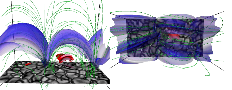
Figure 1: A 3D snapshot of the 3D MHD model in a “$xz$” view (left panel) and “$xy$” view (right panel) at time $t=1200$ s. The blue-red isosurface is at temperature $T=1.4\,10^{6}$ K, where blue for low density plasma ($\approx 8\,10^{-16}$ gr cm^-3) and red for high density plasma ($\approx 10^{-14}$ gr cm^-3). The photospheric continuum intensity is shown with the grey colortable, and some selected magnetic field lines are shown in green to give an indication of the magnetic field topology in the corona.

The computational domain stretches from the upper convection zone to the lower corona and is evaluated on a non-uniform grid of $512\times 256\times 360$ points spanning $16\times 8\times 16$ Mm³ implying a horizontal grid size of $31$ km. The frame of reference for the model is chosen so that $x$ and $y$ are the horizontal directions (see Fig. 1). The grid is non-uniform in the vertical $z$-direction to ensure that the vertical resolution is good enough to resolve the photosphere and the transition region with a grid spacing of $28$ km, while becoming larger at coronal heights where gradients are smaller.

The initial model is seeded with magnetic field, which rapidly receives sufficient stress from photospheric motions to maintain coronal temperatures in the upper part of the computational domain, in the same manner as first done by Gudiksen & Nordlund (2004). The model has an average unsigned field in the photosphere of $160$ G. The magnetic field is distributed in the photosphere in two “bands” of vertical field centered around roughly $x=7$ Mm and $x=13$ Mm. In the corona this results in loop shaped structures, mostly oriented in the $x$-direction, that stretch between these bands as shown in Fig. 1.

We gradually increase the magnetic flux in the atmosphere in order to increase the coronal temperature since the coronal heating in this model occurs when stressed magnetic fields relax. The amplitude of the magnetic field is varied by the following expression:

$${\bf B_{new}}={\bf B_{ini}}(1+\delta/\tau)$$ (1)

where ${\bf B_{ini}}$ is the initial magnetic field in the box, and $\delta$ is the increment in the magnetic field flux, increasing every $\tau$ time interval. Typically, $\delta=5\times 10^{-4}$ and $\tau=1$ s: this time scale is large enough to let the model to relax and reach equilibrium conditions before the next increase occurs. Thus, during the 1500 s of the simulation, the magnetic field increases by a factor $0.75$.

2.1 Synthetic data from SDO/AIA channels

To analyze the emergent emission of the simulated atmosphere, we calculate synthetic images for the various SDO/AIA channels. The emission in each channel is calculated by computing the emission in all lines lying in the corresponding narrow wavelength range of channel sensitivity, folding the resulting spectrum with the wavelength response of the channel and integrating in wavelength. This is done for each vertical column in the numerical domain. The emission for each line is calculated assuming the optically thin approximation under ionization equilibrium conditions. Therefore, the intensity in a spectral line is calculated as follows:

$$I(S)=\int_{l}A_{b}\,n_{\rm e}(V)^{2}G(T(V),n_{\rm e}(V))dl.$$ (2)

where $l$, $S$, and $V$ are length, area, and volume, respectively. In our calculations we obtain AIA synthetic images by integrating ($l$) along the $z$ axis, therefore $S$ is the area in the $xy$ plane. $A_{b}$, $n_{\rm e}$, and $G(T,n_{\rm e}$) are the abundance of the emitting element, the electron density and the contribution function, respectively. The electron density is calculated using the Saha-Boltzman equation. We create a lookup table of the contribution function ($G(T)$ or $G(T,n_{\rm e})$) using the solarsoft package for IDL ch_synthetic.pro, where the keyword GOFT is selected. In general, we calculated the emission taking into account the density dependence of the transition, i.e., using a contribution function $G(T,n_{\rm e})$ instead of $G(T)$. In cases where we use $G(T)$ (see appendix C), a constant pressure is assumed ($P=10^{15}$cm³K). Knowing the temperature ($T$), and the electron density ($n_{\rm e}$) for each grid-point, $G(T,n_{\rm e}$) is obtained by interpolation in the lookup table. We do not calculate the chromospheric emission; the coolest ion that we take into account is He II with a formation temperature $\log(T)=4.9$. To synthesize the plasma emission we use CHIANTI v.6.0.1 (Dere et al., 2009) with the ionization balance chianti.ioneq, available in the CHIANTI distribution. The characteristics of the SDO/AIA channels studied in the present work are listed in table 1. We synthesized AIA observations for two different sets of abundances: photospheric abundances (Grevesse & Sauval, 1998), and coronal abundances (Feldman, 1992). We discuss in detail the effect of abundances in appendix B but in the rest of the main text we will discuss results obtained assuming photospheric abundances, unless noted otherwise.

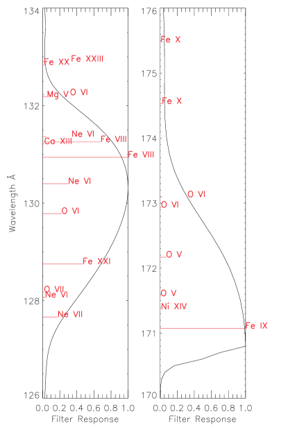
Figure 2: Instrument response as a function of wavelength for the 131 (left panel) and 171 Å (right panel) channels. These responses are available in the solarsoft package for IDL (aia_get_response.pro). The various spectral lines contribution within the passband are shown and labeled, and the length of the red line for each transition is proportional to the maximum of the contribution function for that transition (${\rm max}(G(T))$) (see Section 2.1 for details of $G(T)$).

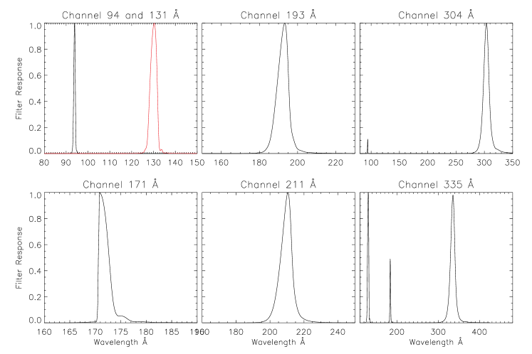
Figure 3: Instrument response as a function of wavelength for the SDO/AIA channels analyzed in this work. SDO/AIA EUV channels 94, 171, 193, 211, 304, and 335 Å are shown from left to right and top to bottom respectively. The response of channel 131 Å is shown in red in the top left panel together with channel 94 Å (shown in black). These response curves are available in the solarsoft package for IDL (aia_get_response.pro).

As shown in Figure 2, where we show the two filters that are amongst the ‘cleanest’, the passband of an AIA filter contains many spectral lines from ions that are different from the dominant ion. We calculate the emission for all lines in the passband of each channel. The wavelength response of the EUV AIA channels are shown in Figure 3. Note that the wavelength responses of the 304 and 335 Å channels have secondary components, i.e., non-negligible sensitivity in spectral ranges far from the central wavelength ($\lambda$) of the passband. This is partly due to crosstalk with the other channel on the same telescope, i.e., the 304 Å channel is contaminated by the 94 Å channel and the 335 Å channel is contaminated by the 131 Å channel. The 335 Å channel also has an additional component due to a higher-order reflection from the multilayer mirror, around 185 Å. Note that the width of the passband (in wavelength) is different for each channel, ordered from narrower to wider: 94, 131, 171, 193, 211, 304, 335 Å. Generally, contributions from a larger set of lines is more likely for wider passbands.

3 Results

3.1 Observational example: quiet sun

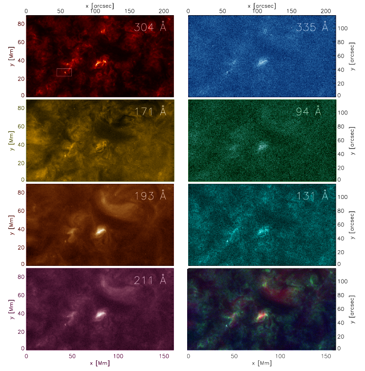
Figure 4: Examples of SDO/AIA images of the quiet sun taken at disk center on 2011 January 7 at 23:50 UT. SDO/AIA channels 304, 171, 193, 211, 335, 94 Å, 131 Å and a composite image with the 304 Å (green), 193 Å (red) and 131 Å (blue) channels are shown, from top to bottom and left to right, respectively. The white square in the top-left panel shows the size of the simulated model.

SDO/AIA observes the full sun continuously with a cadence of $\sim 12$ s and at high spatial resolution ($0.6$ arcsec/pixel). Examples of recent AIA observations in the EUV channels that we simulate are shown in Figure 4. These data are observations of a quiet sun region at disk center on 2011 January 7 around 23:50UT.

The passbands of EUV narrowband imaging instruments are often chosen to contain a dominant single strong emission line or lines from the same ion. Under these conditions, interpretation of the observations is much simplified, as it can be assumed that most of the emission corresponds to the dominant transition and is formed in a definite and narrow temperature range. However, in Figure 4, one can note that some features are similar in most channels, suggesting that the same plasma is the source of the emission in all these channels. An example of such a feature is the bright point centered in the white box in the top-left panel. Given the broad range of temperatures covered by the dominant ions, this could mean that the plasma in the similar-looking feature has a very broad thermal distribution. Alternatively, the presence of lines from non-dominant ions in most of the AIA passbands could, in principle, conspire to “contaminate” all passbands with emission from one or a few ions that are formed at a narrow temperature range that is different from what is expected from the canonical temperature values for the passbands. Here we investigate the importance of the contribution of lines other than the dominant lines for a range of plasma conditions.

3.2 Plasma stratification in the 3D model

As mentioned in section 2, we gradually increase the magnetic flux in the model in order to increase the magnetic field stresses. This leads to a gradual increase with time of the average coronal temperature. In order to simulate SDO/AIA observations in different average plasma conditions, we select three different instants from the time-dependent model, at $t=[800,1200,1460]$ s. The histogram of coronal temperatures at each of the three times is shown in Figure 5; at $t=800$ s the histogram peaks at $T=1.3$ MK, at $t=1200$ s around $1.7$ MK, and at $t=1460$ s the peak is at a temperature above $2$ MK. This hottest atmosphere has a maximum temperature of $\sim 2.8\,10^{6}$ K. The range of temperatures encountered in these different snapshots are likely representative of solar conditions in a coronal hole ($t=800$ s) and quiet Sun, with small hotter emerging regions ($t=1200$) and with a hotter corona (1460 s).

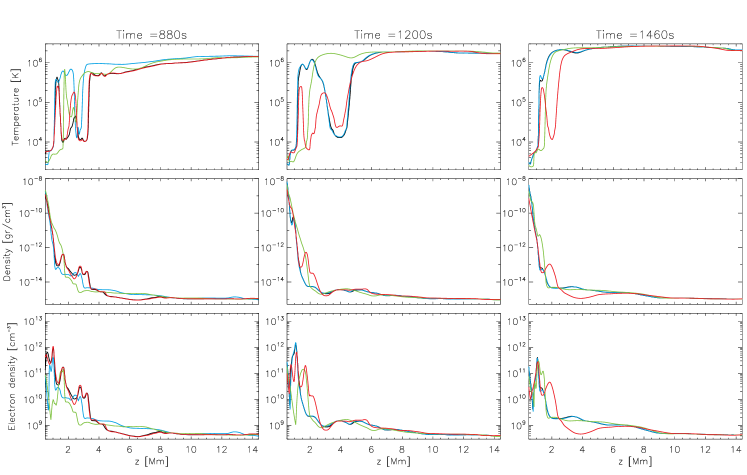
Figure 6: Temperature, density and electron density as a function of height are shown in each row from top to bottom, respectively. The columns from left to right are at time 880, 1200 and 1460 s, respectively. The red, blue, green and black lines correspond to the positions in $x$ and $y$ that are marked with, respectively, dashed red, solid red, dashed green and solid green crosshairs in Figure 7.

Due to the various thermo-dynamics processes and the natural evolution of the model, the temperature, density and electron density stratification vary considerably in both space and time, as shown in Figure 6 where selected ‘columns’ of these variables are plotted as a function of height $z$, for the three times used in this study.

The stratifications presented in Figure 6 show substantial differences. For instance, some of the stratifications show a sharp transition region (green and black lines in the right panels). Other stratifications show cold and dense loops (red lines in the left panels). Moreover, a hot dense loop emerges into the corona around t=1200 s (blue and black lines in the middle column). One can appreciate this highly dense and hot loop in the 3D images in Figure 1. The physical processes and the temporal evolution clearly differ in the different columns. Since these processes are not the main interest in this work, we will not describe them in detail here. However, discussions of similar simulations and the physical processes that govern them can be found in Hansteen et al. (2007) and other papers. For instance, the propagating shocks which lead to type i spicules have been studied in detail by Hansteen et al. (2006); De Pontieu et al. (2007) and Martínez-Sykora et al. (2009). Hansteen et al. (2010) observed from their realistic 3D simulations a distribution of red-shifts with temperature that looks very similar to observations, and found that a heating mechanism that leads to episodic heating events in the vicinity of the upper chromosphere, transition region and lower corona naturally leads to a strong velocity gradient (Martínez-Sykora et al., 2011). An important source of plasma injection into the corona are the jets and type ii spicules (Heggland et al., 2009; Martínez-Sykora et al., 2011). In addition, the emergence of magnetic flux into the corona has been described by Martínez-Sykora et al. (2008, 2009).

We will show in the following sections that as a consequence of these and similar processes and their resulting stratifications, the emission in the SDO/AIA channels may often come from non-dominant ions and/or from plasma that is significantly cooler or hotter than the formation temperature of the dominant ion(s).

3.3 “Narrow” filter passband description

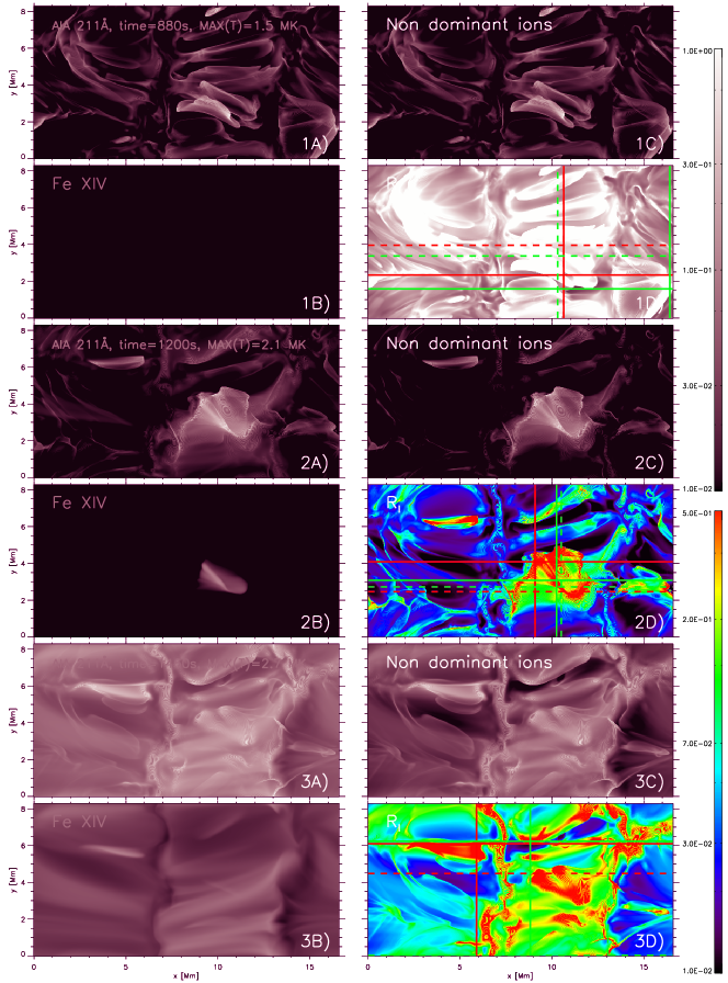
Figure 7: Synthetic images of channel 211 Å. This collection of panels are set in three groups of four panels. Each group is set a different time (880, 1200 and 1460 s) which are shown in the panels labeled 1A-D, 2A-D and 3A-D, respectively. In each set of four panels, we show $I_{T}$, $I_{D}$, $I_{ND}$ and $R_{I}$ in panels labeled 1-3A, 1-3B, 1-3C, and 1-3D, respectively. The synthesized intensities have been normalized to the maximum intensity of the synthesized SDO/AIA channel (panels 1-3A) and all use the same color scheme in logarithmic scale (top colorbar). The color scheme for $R_{I}$ is shown with the bottom colorbar in logarithmic scale. The solid red, dashed red, solid green and dashed green crosshairs in panels 1-3D are the locations in $y$ corresponding to the panels labeled 1-3a, 1-3b, 1-3c and 1-3d in Figure 8 and in Movie 2.

While we discuss all SDO/AIA channels in this section, we only show figures for one channel in the main paper (211 Å  see Figure 7-9). However, similar figures for all channels can be found in the on-line version of the paper (Movies 1-3). Figure 7 and the equivalent figures in Movie 1 are composed of three groups of four panels. Each group corresponds to a different snapshot in time (labeled as 1A-D, 2A-D and 3A-D at times 880, 1200 and 1460 s, respectively). As mentioned, these three different snapshots have coronae with very different temperature distributions; in general the coronal temperature increases with time as shown in Figure 5. The four panels of each group (or each image in Movie 1) show: the total synthesized emission ($I_{T}$, labeled with “A”), the intensity emitted by the dominant ion(s) ($I_{D}$, labeled with “B”), the intensity emitted in spectral lines of non-dominant ions ($I_{ND}$, labeled “C”), and the ratio $R_{I}$ (labeled with “D”). For each SDO/AIA channel, $R_{I}$ is the ratio between the emission from the non-dominant ions and the emission from the dominant ion(s), weighted with the synthesized intensities for the specific channel, as defined in the following expression:

$$R_{I}=\frac{I_{ND}}{I_{D}}I_{T}$$ (3)

The color scale for the panels 1-3D is shown at the bottom-right of Figures 7, or at the top-right in the movies. Orange-red colored areas correspond to regions where the emission from the non-dominant ions is relatively large compared to the emission from the dominant ions, and in addition where the total emission of the synthesized channel is significant. The color-scale for panels 1-3A, B and C is shown in the top-right of Figure 7 or the top-left of Movie 1. The color-scheme of this color bar changes from channel to channel, to allow easier identification of the channels in Movies 1, 3, 4, 5, and 6. We use the same color schemes as those of the SDO/AIA webpages (http://sdo.gsfc.nasa.gov/data/). These color schemes can be loaded using the solarsoft routine aia_lct.pro.

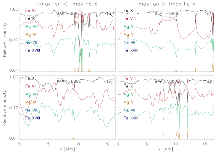
Figure 8: Relative contribution for the most significant spectral lines in the 94 Å channel, at time 880 s for four specific $y$-positions in the field of view. The ions listed in each plot are those with the most important contributions, ordered from the largest to the smallest contribution (from top to bottom). Each panel shows a different $y$ position, which is marked with a crosshair in panel 1D of Figure 7. The solid and dashed red, and solid and dashed green crosshairs are shown in the panels labeled 1a, 1b, 1c, and 1d in this figure, respectively.

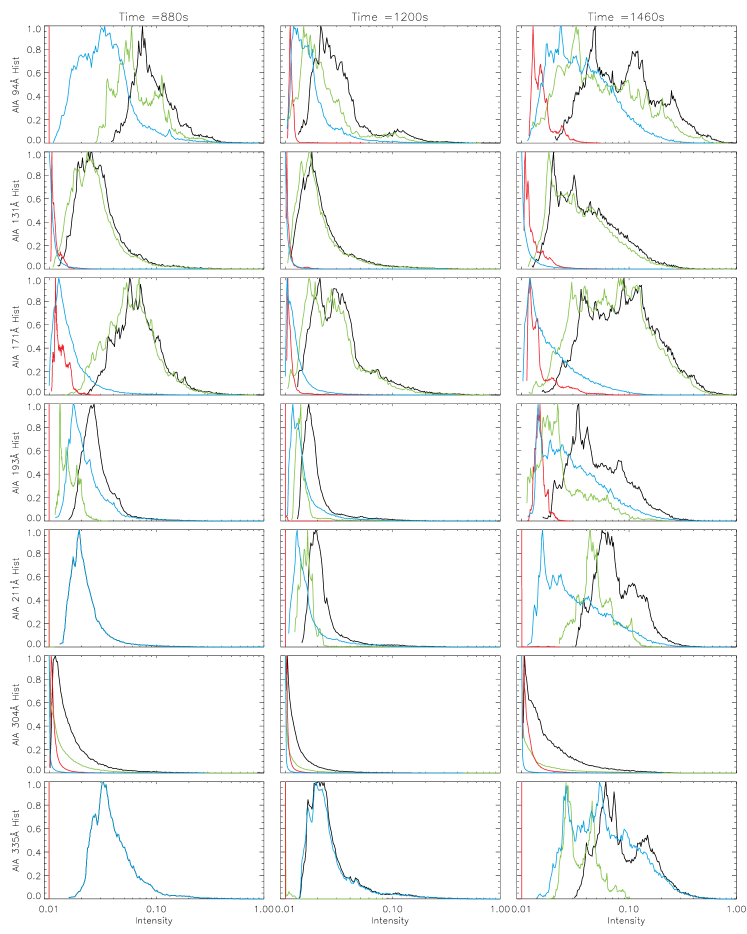
Figure 10: Histograms of the intensities $I_{L}$, $I_{H}$, $I_{I}$, and $I_{T}$ are shown in blue, red, green and black lines. The columns are at the timesteps 880 s, 1200 s and 1460 s from left to right, and the rows are the different SDO/AIA channels.

Before discussing in detail the plots shown in Figures 7, and Movie 1 for each channel, we describe Figures 8 and 9 and the corresponding Movies 2 and 3, and Figures 10 and 11. In Figure 8, and in each image in Movie 2, we plot the relative contribution of the most significant spectral lines from the various ions within a passband. This shows how much emission comes from each ion (normalized to the total emission) in a given filter for a specific $y$-position. In each plot we list the ions with the most significant contributions, ordered from the one with the largest relative contribution along the x-axis (top) to the one with the lowest relative contribution (bottom). In order to clarify: if the emission only came from the dominant ion, its relative contribution would be equal to one everywhere. We show results for four different $y$-positions within the field of view (one per panel). The different positions in $y$ are marked with differently colored and styled crosshairs in the panels 1-3D in Figure 7 and in Movie 1. The relative contribution for the locations marked by the solid red, dashed red, solid green and dashed green crosshairs are shown in the panels labeled 1-3a, 1-3b, 1-3c and 1-3d in Figure 8 and in Movie 2. We define $I_{NDL}$ as the intensity coming from the non-dominant ions that have a peak formation temperature lower than that of the dominant ion, and $I_{NDH}$ as the intensity coming from the non-dominant ions which have a peak formation temperature higher than that of the dominant ion. With these definitions, the location of each crosshair is then selected as follows: the solid red crosshair is where $(I_{NDL}/I_{D})I_{T}$ is largest, i.e., most of the emission comes from ions that have formation temperatures lower than the dominant ion (at locations where the emission is not negligible); dashed red crosshair is where $I_{NDL}/I_{D}$ is largest, i.e., most of the emission comes from ions that have formation temperatures lower than the dominant ion; solid green crosshair is where $(I_{NDH}/I_{D})I_{T}$ is largest, i.e., most of the emission comes from ions that have formation temperatures higher than the dominant ion (at locations where the emission is not negligible); and dashed green crosshair is where $I_{NDH}/I_{D}$ is largest, i.e., most of the emission comes from ions that have formation temperatures higher than the dominant ion (see Table 2).

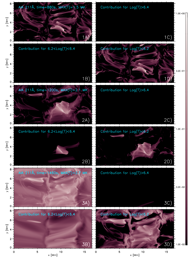
Figure 9: Emission contribution for different temperature ranges for the synthesized 211 Å emission is shown at $t=880$ s (panels labeled 1A-D), $t=1200$ s (panels labeled 2A-D), and at $t=1460$ s (panels labeled 3A-D). The synthesized intensities $I_{T}$, $I_{I}$, $I_{H}$, and $I_{L}$ are shown in the panels labeled 1-3A, 1-3B, 1-3C and 1-3D, respectively (see text for definition). The color-scheme is shown in the right colorbar in logarithmic scale and all panels are normalized to the maximum of the synthesized intensity (panels 1-3A).

Using the same synthetic calculations, we can look at the same data, but categorize the emission for each channel as a function of temperature of the emitting plasma, instead of in terms of the “dominant” and “non-dominant” ions. Figure 9 shows the emission coming from various temperature ranges in the model for the 211 Å channel at $t=880$ s (top four panels labeled 1A-D), at $t=1200$ s (middle four panels labeled 2A-D), and at $t=1460$ s (bottom four panels labeled 3A-D). Each group of four panels and each image in Movie 3, where we present similar plots for the other channels, has the same layout. The synthesized image for the specific channel is shown in the panels labeled 1-3A. For each passband three temperature ranges are defined. The emission is then calculated, taking into account all the various spectral lines within the passband. The intensity coming from plasma at temperatures where the $G(T,n_{\rm e})$ of the dominant ion is larger than $1/e$ of its maximum is shown in the panels 1-3B ($I_{I}$). For example, for the 211 Å channel the corresponding temperature range is $6.2<\log(T)<6.4$ (see Figure 9). For the channels with more than one dominant ion, we choose the dominant ion which has the lowest formation temperature, since the temperatures of our model are in the lower range of coronal temperatures observed on the sun. Panels 1-3C show the intensity $I_{H}$ coming from plasma at temperatures higher than the high temperature value where the $G(T,n_{\rm e})$ of the dominant ion is $1/e$ of its maximum, e.g., for the 211 Å channel $I_{H}$ is the intensity of emission from plasma at temperatures higher than $\log(T)=6.4$. Finally, panels 1-3D show the intensity $I_{L}$ coming from plasma at temperatures lower than the low temperature value where the $G(T,n_{\rm e})$ of the dominant ion is $1/e$ of its maximum, e.g., from plasma at temperatures lower than $\log(T)=6.2$ for the 211 Å channel.

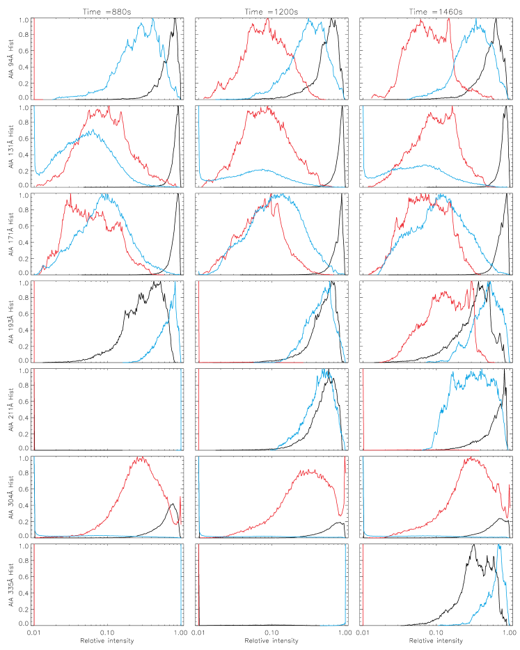
Figure 11: Histograms of the relative contribution from $I_{L}$/$I_{T}$, $I_{H}$/$I_{T}$, and $I_{I}/I_{T}$ are shown in blue, red and black lines. The columns are at the timesteps 880 s, 1200 s and 1460 s from left to right, and the rows are the different SDO/AIA channels.

In order to quantify the dependence of the emission with temperature we show Figures 10 and 11. Histograms of the intensities and the relative intensities coming from different temperature ranges are shown in Figure 10 and Figure 11, respectively. The histograms of the intensities $I_{L}$, $I_{H}$, $I_{I}$, and $I_{T}$ are shown with blue, red, green and black lines in Figure 10. When the green line is close to the black line, most of the emission for a specific channel comes from temperatures near the formation temperature of the dominant ion. These histograms are shown for each channel (rows) and at the three different instants; $t=880,1200,1460$ s (columns).

The histograms of the relative intensities $I_{L}$/$I_{T}$, $I_{H}$/$I_{T}$, and $I_{I}/I_{T}$ are shown with blue, red and black lines in Figure 11. As in Figure 10, the columns are for the timesteps $t=880,1200,1460$ s from left to right, with the different SDO/AIA channels in different rows. Note that when the black histogram is concentrated on a relative intensity of 1, all the emission comes from temperatures near the formation temperature of the dominant ion. When the black histogram is more spread out, other temperature ranges also contribute significantly to the passband.

As shown in detail in the appendix A, we also investigated the effect of the instrumental spatial resolution by degrading the synthetic emission to the AIA spatial resolution. In summary, we found that the detailed description given for each channel below is also valid when the synthesized intensities are convolved and pixelized to the SDO/AIA resolution. However, the smaller structures disappear or are mixed with emission coming from other structures.

3.3.1 94 Å channel

The SDO/AIA 94 Å channel has emission from two dominant ions with rather different formation temperatures; Fe X at $10^{6}$ K and Fe XVIII at $6\times 10^{6}$ K (see Table 1). Moreover, there is some evidence suggesting that this passband contains emission from some lines that are not included in CHIANTI (e.g., Testa et al., 2011; Foster et al., 2011; Schmelz et al., 2011; Aschwanden & Boerner, 2011), therefore our analysis of the contributions to the 94 Å emission might be inaccurate. However, until the impact of these missing transitions will be assessed and their emission properly modeled and included in the atomic databases, the interpretation of AIA 94 Å observations will be based on existing atomic data, and therefore we believe that our investigations using the CHIANTI database are relevant for present AIA studies. Our model does not reach extremely high temperatures, so very little emission comes from the Fe XVIII lines. As a result, we consider Fe X as a dominant ion. At any given time non-dominant ions contribute significantly changing both the total intensity and shape of observed features (see panels 1-3C and 1-3D in Movie 1 for the corresponding channel). For example, at time $t=1200$ s (panels 2A-D), a bright emerging loop appears roughly in the center of the image. This structure shows a significantly different intensity in the synthesized 94 Å channel (panel 2A in Movie 1 for the corresponding channel) as compared to the intensity from the dominant ions (see panel 2B). This is because the loop has a strong contribution from ions with formation temperatures cooler than that of the dominant ions (see left panels in the corresponding image in Movie 2). Note that while the intensity is different, the shape of this emerging hot dense loop is similar in both images (panels 2A and 2B in Movie 1).

The non-dominant ions that provide the most important contributions to the 94 Å emission are different from gridpoint to gridpoint and from timestep to timestep due to the highly dynamic nature of the atmosphere. This can be seen in the corresponding snapshots of Movie 2. It is important to remark that the relative contribution of each ion changes considerably for different positions in space in the same snapshot (i.e., at the same instant). For instance, panels 1-3a and 1-3b in Movie 2 include the position where non-dominant ions that have formation temperatures lower than the dominant ion provide strong contributions to the emission. In these positions, the most important ion is Fe VIII. Emission from other ions is at least one order of magnitude smaller than the emission coming from the dominant ion with, in order of importance, Mg VIII, Mg VI, and Ne VII. The dominant ion Fe X in these positions is also one order of magnitude smaller than the most important ion (Fe VIII). Panels 1-3c and 1-3d in Movie 2 include the locations where non-dominant ions with formation temperatures higher than the dominant ion provide strong contributions, i.e., $(I_{NDH}/I_{D})I_{T}$ and $I_{NDH}/I_{D}$ are highest. In these positions, the most important ions are Fe VIII, Fe X, Mg VIII, Mg VI, and Ne VII in order of importance, at the first timesteps (1a-d and 2a-d in Movie 2). Note that Fe VIII, Mg VIII, Mg VI, and Ne VII have a formation temperature lower than of the dominant Fe X ion, i.e., in locations where hotter ions play the most important role they are still insignificant compared to the ions with a lower temperature formation taking into account the temperature range of the simulation.

It is interesting to note that the relative contribution from the various ions varies by orders of magnitude in space (as shown, e.g., in the horizontal direction along $x$ in Movie 2). Therefore, when we observe the Sun, the most important relative contribution to this channel may be from different ions depending on exactly when and where we are looking, and can be very different at locations only a few pixels apart. When the model gets hotter, a different set of ions become more important (3a-d, Movie 2), such as Fe XVIII. However, the impact of the non-dominant ions is generally less important when the model reaches higher temperatures (compare the panels 3A-D with the panels 2A-D and 1A-D in Movie 1). In sumary, the most important ion in the channel varies between Fe VIII, Fe X, and Fe XVIII, with the other ions having contributions that are for the most regions one order of magnitude smaller.

In panels 1-3B of Movie 3 we show the emission in the 94 Å channel from the plasma with a range in temperature of $\log(T)=[5.9,6.2]$. At $t=880$ s, an important contribution to the emission comes from plasma at temperatures cooler than $\log(T)=5.9$ (see panel 1C in Movie 3). This emission is significant enough to impact the total synthesized intensity. As a result, some features that are observed in the emission from the range of temperatures $5.9<\log(T)<6.2$ have a different shape and intensity in the synthesized image of the AIA channel (panels 1A in Movie 3). Comparing panels 2A-D and 3A-D with panels 1A-D it is clear that the influence of plasma cooler than $\log(T)=5.9$ is less pronounced at later times. Most of the contributions at temperatures cooler than $\log(T)=5.9$ are due to non-dominant ions which have formation temperatures lower than that of the dominant ions Fe X and Fe XVIII.

There is no emission coming from plasma at temperatures larger than $\log(T)=6.2$ at $t=880$ s (see panel 1C in Movie 3) since the model does not reach temperatures greater than $\log(T)=6.2$ at this time. Later, when the model has reached temperatures that are larger than $\log(T)=6.2$, such emission exists, but is generally negligible (see panels 2-3C in Movie 3 and top row in Figure 10).

Figures 10 and 11 quantify the emission coming from the various temperature ranges. Most of the values for the normalized intensity $I_{T}$ are of order 0.08, 0.02, and 0.05 of the maximum intensity in the box at times 880 s, 1200 s, and 1460 s, respectively (see the black line in the top row in Figure 10). At time 1200 s, the emerging loop shows very strong emission which pushes the maximum intensity in the box to very high levels. As a result, most of the normalized intensities are quite small compared to its maximum, hence the shift of the black histogram towards smaller values.

Ideally, when all the emission comes from within the temperature range $\log(T)=[5.9,6.2]$, the green lines coincide with the black lines. However, in this channel, the black line is mostly a combination of the green and blue line, i.e. the emission stems from plasma at the temperature of the dominant ion and cooler. Most of the intensity coming from temperatures between $5.9<\log(T)<6.2$ is at levels of 0.07, 0.015, and 0.03 of the maximum intensity at time 880 s, 1200 s and 1460 s, respectively (see green lines in the first row in Figure 10). The intensity coming from temperatures lower than $\log(T)=5.9$ is found mostly to have values of 0.03, 0.012 and 0.02 of the maximum at time 880 s, 1200 s and 1460 s, respectively (see blue lines in the first row in Figure 10). Contribution of cold plasma (blue lines) is roughly half of the contribution of the plasma at temperatures typical of the dominant ion (green lines). Therefore, the number of points emitting at intensities around the maximum in the histogram at time 880 s (black lines) is roughly 50% larger than green line. For larger intensities (i.e., brighter regions), at all instants, this difference between the green and black lines is smaller. In the first row in Figure 11 one can observe that in general $1/3$ or more of the emission comes from cold plasma (blue lines) and $2/3$ from the range of temperatures $5.9<\log(T)<6.2$ (black lines).

In appendix B we compare the emission using photospheric and coronal abundances. This channel shows wide areas where the emission is different by assuming photospheric or coronal abundances, reflecting the ratio of the abundance between the two datasets where Fe is different from Ne, which these two ions contribute to the emission. In appendix C we study, for each channel, the dependence of the emission on the electron density. The 94Å channel shows some significant dependence on the electron density because the Fe X 94 Å line is density sensitive and contributes significantly to the emission.

In summary, the emission from cooler plasma plays a role everywhere at all times in this channel, but it typically contributes less in brighter and hotter regions.

3.3.2 131 Å channel

The SDO/AIA 131 Å channel has emission from two dominant ions which are formed at completely different temperatures: Fe VIII at $6\times 10^{5}$ K and Fe XX at $10^{7}$ K; however, in non-flaring conditions emission from the very hot Fe XX ion is negligible. The various structures observed in the synthetic 131 Å channel (panels 1-3A in Movie 1) are similar to those seen in the emission from the dominant ion (panels 1-3B in Movie 1). Due to the temperatures that the model reaches, the dominant ion producing the most emission is Fe VIII. At the same time, some of the emission from the non-dominant ions does have a small impact in the synthesized intensity of this AIA channel, depending on where and when we are observing in the model. This can be seen when one compares the synthetic 131 Å image (panels 1-3A in Movie 1) and the emission coming from the dominant ions (panels 1-3B in Movie 1).

In contrast to the previous passband, in the 131 Å channel the contribution from Fe VIII is dominant always and everywhere (Movie 2). However, in a few places O VI and Ne VI have a relative contribution that is comparable with that of the dominant ion. Other ions that play some role in this filter are Ne VII and Mg V, but with relative contributions one order of magnitude smaller than the dominant ion. Note that most of these ions have formation temperatures lower than the dominant ion Fe VIII. However, later in time (panels 3c-d in Movie 2), in addition to the ions mentioned, ions with formation temperatures hotter than Fe VIII contribute to the total intensity. These include Si XII, O VII, Si XI, and Ca XIII, which have contributions up to one order of magnitude smaller than the contribution from Fe VIII in a few locations at time 1460 s (panels 3c-d in Movie 2). Note that in some places the intensity signal appears “noisy”. This occurs in places where the emission comes from transition region plasma: in the transition region, the temperature gradient is large, causing large jumps in temperature between grid points so that the interpolation with $G(T,n_{\rm e})$ gives a noisy signal.

In panels 1-3B of Movie 3 we show emission in the 131 Å channel from plasma within the temperature range $\log(T)=[5.5,6]$. At all timesteps, most of the emission comes from temperatures between $5.5<\log(T)<6$ (see panels 1-3B in Movie 3). The contributions from cooler (panels 1-3D) or hotter (panels 1-3C) plasma is almost negligible at all instants and almost everywhere. However, in a few small areas, some faint emission is produced by both cooler ($\log(T)<5.5$; see panels 1-3D) and hotter ($\log(T)>6$; see panels 2-3C) plasma. The latter is appreciable only when the model reaches high enough temperatures, i.e., at times 1200 s and 1460 s.

Most of the normalized intensities $I_{T}$ are of the order 0.025, 0.018, and 0.02 of the maximum intensity at times 880 s, 1200 s, and 1460 s, respectively (see the black line in the second row in Figure 10). As mentioned for the 94 Å channel, at time 1200 s the emerging loop shows very strong emission. As a result most of the normalized intensities show small values at this time. (This behavior is also observed in the other channels, with the exception of the 211 and 335 Å channels, as discussed below). For most of the intensities, the black line is similar to the green line, i.e., for the rather restricted variation of atmospheric temperatures in the model, we can conclude that, for any range of intensities, the emission in this channel comes from plasma with a temperature range $\log(T)=[5.5,6]$. This is confirmed by the second row in Figure 11 where we can observe that in general most of the emission (in each pixel) comes from plasma at temperatures $5.5<\log(T)<6$ (black lines), while only 10% of the emission arises from hotter plasma.

As shown in detail in appendix B, for the 131 Å channel, at all instants, the intensity calculated with the photospheric abundances is between 2.5 and 3.3 times smaller than the intensity calculated with the coronal abundances. This is caused by the different relative abundances of O and Ne, with respect to Fe, in the two datasets. The contributing ions, O VI, and Ne VI/VII, have peak formation temperatures similar to the dominant ion, Fe VIII. So the temperature dependence of the relative contribution of the different elements is less pronounced in the 131 Å channel than in the other channels. As described in detail in appendix C, the emission in this channel is not density sensitive.

In summary, at least for the temperature regimes covered by the model, the dominant ion producing the most emission is Fe VIII. The emission coming from other ions or/and plasma with temperatures that differ from the peak temperature formation of Fe VIII is faint.

3.3.3 171 Å channel

The SDO/AIA 171 Å channel has emission from two dominant ions, Fe IX and Fe X, which have similar formation temperatures; $7\times 10^{5}$ K and $10^{6}$ K. As in the 94 Å channel, the structures observed in the synthesized 171 Å channel (panels 1-3A in Movie 1) are similar to those seen in the emission coming from dominant ions (panels 1-3B in Movie 1). Most of the time this channel is dominated by Fe IX. However, as in the 131 Å channel, the importance of the non-dominant ions varies significantly both in space and time. This can be observed clearly in Movie 2 which shows which ions contribute to the total intensity.

The most important cool non-dominant ions are O V and O VI. In a few locations, emission from O V is sometimes one order of magnitude larger than the emission coming from the Fe IX ion, with emission from O VI of the same order of magnitude as the Fe IX ion. However, in most locations, the emission from the dominant ions is the most important, by almost two orders of magnitude compared to the emission coming from the other ions. Fe X plays a small but still rather important role in this filter. Later in time, when the model is hotter, additional ions contribute as much as Fe X, such as Ni XIV and Ar X, which have a higher formation temperature than Fe X (see panel 3b-d in Movie 2).

In the 171 Å channel, the range in temperatures where the $G(T,n_{\rm e})$ of the dominant ions Fe IX is larger than $1/e$ of its maximum is $\log(T)=[5.7,6.1]$. The impact of the emission coming from plasma that is hotter (panels 1-3C in Movie 3) or cooler (panels 1-3D) than the range $\log(T)=[5.7,6.1]$ is similar to that observed in channel 131 Å. At all timesteps, most of the emission comes from temperatures within $5.7<\log(T)<6.1$ (see panels 1-3B in Movie 3) which is produced mostly by the dominant ions. The effects from hotter plasma are almost negligible at all instants and almost everywhere (panels 1-3C). Even when the model reaches higher temperatures (i.e., at times 1200 s and 1460 s) these lines only provide a rather weak contribution. The contribution coming from plasma cooler than $\log(T)=5.7$ has only a limited impact (see panels 1-3D in Movie 3): it does not change the intensity much, nor does it change the shapes of structures seen in the synthesized intensity of this channel at any time.

Most of the normalized intensity $I_{T}$ values are around 0.06, 0.02, and 0.1 of the maximum intensity at times 880 s, 1200 s, and 1460 s, respectively (see the black line in the third row in Figure 10). Similarly to what we found for channel 131 Å, the black line is overall close to the green line. Therefore, when the atmospheric temperatures vary within the model, one can conclude that, at any range of intensities, the emission from this channel comes from the temperature range $5.7<\log(T)<6.1$ (green line).

This is confirmed by the third row in Figure 11 where we can observe that in general most of the emission in each pixel comes from the range of temperatures $5.7<\log(T)<6.1$ (black lines). Only slightly more than 10% of the emission comes from plasma cooler than $\log(T)=5.7$ and slightly less than 10% of the emission comes from plasma hotter than $\log(T)=6.1$.

As shown in detail in appendix B, the differences in emission between the two datasets with different abundances (photospheric and coronal) arise from the differences in Fe abundances between both datasets. There are also small and narrow areas where the emission is different because emission from elements other than Fe is substantial (e.g. O V/VI, and Ne IV/V).

As shown in detail in appendix C, the emission from some structures shows a dependence on the plasma density, especially at later times (t=1200 and 1460 s). This is mainly due to the sensitivity to density of the strong Fe IX 171 Å spectral line. In addition, other lines which contribute less to the emission have also a strong dependence on density, e.g., Fe X 170 Å, O V 171 Å, and Ni XIV 171 Å.

In short, our analysis indicates that the emission coming from other ions or/and plasma with temperatures that differ from the peak temperature formation of Fe IX/X is rather faint.

3.3.4 193 Å channel

The dominant ion in the SDO/AIA 193 Å channel is Fe XII which is formed at $\sim 1.2\times 10^{6}$ K. However, this synthesized channel is influenced by the non-dominant ions in a similar manner as the 94 Å channel. Therefore, the various structures observed in the synthesized 193 Å emission (panels 1-3A in Movie 1) are different both in morphology and intensity as compared to the emission coming from the dominant ion (panels 1-3B in Movie 1). The contributions to the emission coming from the non-dominant ions is rather important at all three instants, i.e., at all temperatures (see red areas in the panels 1-3D in Movie 1).

The contributions of the most important non-dominant ions vary strongly in time and space (see Movie 2), and are mainly due to O V and Fe VIII, which are of the same order as Fe XII. While the relative contributions of Fe IX and Fe XI are an order of magnitude smaller than Fe XII in most locations, they are significant in some locations. In addition, a relative contribution of one order of magnitude smaller than that of the most important ion(s) comes from Fe X, S XI, Fe XIII and Ar X. In some places the emission comes from cooler plasma (transition region) as can seen from the “noisy” signal.

In the 193 Å channel, the range in temperatures where the $G(T,n_{\rm e})$ of the dominant ion is larger than $1/e$ of its maximum is $\log(T)=[6.1,6.3]$. Since the model has relatively low temperatures, most of the emission in this channel comes from plasma at temperatures lower than $\log(T)=6.1$, corresponding to emission from non-dominant ions which have a formation temperature that is lower than the dominant ion (see panels 1-3D in Movie 3). As seen above, the 171 Å shows a similar behavior. It is interesting to note that, even at the later times, when the model has sufficiently high temperatures, most of the emission comes from plasma that is cooler than $\log(T)=6.1$ in this channel. Note also that the structuring and intensities produced by the various ranges of temperature are completely different. This is because, at all instants, the sources (ions) emit in different regions (compare to panels 1-3B, 1-3C and 1-3D in Movie 3). The emission from plasma at temperatures higher than $\log(T)=6.3$ is negligible at all instants. At $t=880$ s, we also see that even the emission from plasma at temperatures $\log(T)=[6.1,6.3]$ is faint. The emission coming from the range of temperature $6.1<\log(T)<6.3$ comes mostly from the dominant ions.

Most of the normalized intensity $I_{T}$ values are around 0.025, 0.018, and 0.033 of the maximum intensity in the box at times 880 s, 1200 s, and 1460 s, respectively (see the black lines in the fourth row in Figure 10). The black lines ($I_{T}$) are mostly a combination of the green ($I_{I}$) and blue ($I_{L}$) lines.

The plasma with temperatures between $6.1<\log(T)<6.3$ typically shows normalized intensity ($I_{I}$) values of 0.014, 0.015, and 0.02 of the maximum intensity in the box at times 880 s, 1200 s and 1460 s, respectively (green lines). Plasma with temperatures lower than $\log(T)=6.1$ ($I_{L}$) shows normalized intensity values of 0.016, 0.012 and 0.015 at times 880 s, 1200 s and 1460 s, respectively (blue lines). We can thus see that the contributions from cooler plasma change with time. For brighter locations, at all instants, the cold plasma (blue lines) emits in more locations than plasma at temperatures $\log(T)=[6.1,6.3]$ (green lines). In the fourth row in Figure 11 one can observe that at time 880 s most of the emission for most of the locations arises from plasma at temperatures lower than $\log(T)=6.1$ (blue lines). However, a large number of locations have strong contributions from plasma at temperatures $6.1<\log(T)<6.3$ (black lines). At time 1200 s the dominance of the emission per pixel is shared between these two ranges of temperatures. Finally, at time 1460 s most of the pixels have more contributions from cold plasma (blue lines). For most locations roughly 30% of its intensity comes from plasma with temperatures $6.1<\log(T)<6.3$ (black lines); and 20% of its intensity comes from plasma hotter than $\log(T)=6.3$ (red lines).

The assumed abundances have a significant impact on the 193Å emission in two ways: 1) in large regions the ratio of the emission calculated using the two different abundances varies smoothly between 1 and 1.7 due to significant contributions from non-Fe ions throughout the field of view; 2) in some small and narrow features this ratio significantly departs from 1 because the relative contribution of emission from elements other than Fe is very substantial (see appendix B for details).

As found for the 94 Å  and 171 Å channels, some structures show a dependence on electron density, because several spectral lines contributing to their emission are density dependent (these lines are listed in appendix C).

In summary, emission coming from other ions (e.g. O V and Fe VIII) or/and plasma with temperatures that are cooler than the peak temperature formation of Fe XII contribute considerably to the total emission.

3.3.5 211 Å channel

The SDO/AIA 211 Å channel has emission from one dominant ion, Fe XIV, which has a peak formation temperature of $\approx 2\times 10^{6}$ MK, i.e. near the upper limit of the temperature range of our model. We can therefore expect that non-dominant ions will play a larger role than in atmospheres with higher average temperatures. Figure 7 illustrates that most of the synthesized emission of channel 211 Å (panels 1-3A) comes from the so-called non-dominant ions (panels 1-3C). The emerging loop seen in channel 94 Å at time 1200 s is also visible in this channel. However, in channel 211 Å this structure in particular, as well as most of the other small structures observed, shows a markedly different shape than that seen in the emission coming from the dominant ion (panel 2B). This is because this channel has strong contributions from ions with cooler formation temperatures (see panels 1-3C and 1-3D in Figure 7 and the corresponding images in Movie 2).

In a similar manner to channel 94 Å, the ions which provide the most important contributions differ from gridpoint to gridpoint due to the dynamic atmosphere (see Movie 2). However, at all instants, all the non-dominant ions significantly contributing to the emission are formed at temperatures lower than the peak formation temperature of the dominant ion. This is presumably because the temperature of the model barely reaches temperatures above the peak formation temperature of the dominant ion. The most important ions in terms of emission are O V and O IV. However, there are other ions that are important contributors as well, depending on the timestep and position in the box. These contributions are due the ions Ne V, Ne IV and N V, Fe XII and Fe XIII (in addition to small contributions from the “dominant” ion Fe XIV).

In the right panels in Movie 2 we see additional ions which also contribute, such as Fe VIII, Si VIII, Ni XI, and Fe X. At $t=880$ s, there are a large variety of contributions coming from various ions. Later in time, at $t=1200$ s, when the coronal plasma is hotter, more integrated columns have a clear dominance of contributions coming from the ions Fe XIV and Fe XIII. This is even more pronounced at $t=1460$ s, where we find a clear dominance by the dominant ion, though even here, not at all locations. The highly dynamic stratification is thus variable enough to considerably change the importance of the emission from each contributing ion.

The range in temperatures where the $G(T,n_{\rm e})$ of the dominant ion is larger than 1/e of its maximum is $\log(T)=[6.2,6.4]$ for the 211 Å channel (see panels 1-3B in Figure 9). The impact of the emission coming from hotter or cooler plasma than this range is similar to the ones observed in channel 193 Å. Therefore, since the model is relatively cold, most of the emission comes from temperatures lower than $\log(T)=6.2$, and its origin is from the non-dominant ions which have a formation temperature lower than that of the dominant ion. This happens at all instants, but when the temperature of the model is high enough, some structures formed at temperatures between $6.2<\log(T)<6.4$ are also observed in the synthesized intensity of the channel. In a similar manner as in channel 193 Å, it is important to note that the shapes of structures and intensities coming from the various temperature ranges are completely different. This is because the sources and regions responsible for the various temperature ranges are physically distinct. The emission coming from plasma at temperatures larger than $\log(T)=6.4$ is negligible. At $t=880$ s the emission coming from plasma with temperatures for which $\log(T)=[6.2,6.4]$ is also faint.

In general, the emission from plasma in the range of temperatures $6.2<\log(T)<6.4$ comes mostly from the dominant ion. However, one can see some structures which are slightly larger or only appear in the intensity emitted by plasma with temperatures $6.2<\log(T)<6.4$. This is clearly visible when comparing the emission coming from this range (Movie 3) with the intensity coming from the dominant ion in Movie 1. These differences arise because the channel has some contributions from the Fe XIII which has a formation temperature relatively close to the dominant ion.

Most of the normalized intensity $I_{T}$ values are around 0.02, 0.02, and 0.07 of the maximum intensity at times 880 s, 1200 s, and 1460 s, respectively (see the black lines in the fourth row in Figure 10). Note that, in comparison with other channels, at time 1200 s the emission from the emerging loop (relative to the rest of the box) is not as strong as in the other channels. At time 880 s, at any value of intensity, the black line ($I_{T}$) is the same as the blue line ($I_{L}$). This means that all the emission comes from cold plasma (blue lines, $I_{L}$). However, later in time, some emission comes from the range of temperatures $\log(T)=[6.2,6.4]$ (green lines, $I_{I}$). This becomes clear when viewing the histogram: most of the normalized intensity values emitted by plasma with temperatures $6.2<\log(T)<6.4$ ($I_{I}$) are 0.0, 0.016, and 0.04 at times 880 s, 1200 s and 1460 s, respectively (green lines). The normalized intensity values emitted by plasma with temperatures lower than $\log(T)=6.2$ are 0.02, 0.013 and 0.016 of the maximum of the box at times 880 s, 1200 s and 1460 s, respectively (blue lines, $I_{L}$). Again we see that the contributions of cold and hot plasma to the intensity in each pixel vary at times 1200 s and 1460 s. It is interesting to see that the intensity histogram from the cold plasma (blue lines) is larger below intensities 0.04 and above intensities 0.1 than the histogram of the intensity emitted by plasma with temperatures $6.2<\log(T)<6.4$ (green lines). Therefore, most of the emission of the weak background comes from cold plasma, but also the strong intensity features come from cold plasma (blue lines).

In the fourth row in Figure 11 one can observe that at time 880 s, for all the integrated columns, all the emission comes from temperatures lower than $\log(T)=6.2$ (blue lines). At time 1200 s, the dominance of the emission per point is shared between temperatures lower than $\log(T)=6.2$ (blue lines) and the range of temperatures $6.2<\log(T)<6.4$ (black lines). Finally, at time 1460 s most of the integrated columns have more contribution from plasma with temperature $6.2<\log(T)<6.4$ (black lines), and for most of them roughly 30% of its intensity is emitted by cold plasma (blue lines).

As found for the 193 Å channel, the difference of the synthetic images assuming photospheric or coronal abundances is “twofold”: 1. in large regions the ratio of the emission calculated using the two different sets of abundances varies smoothly; 2. there are small and narrow features where this ratio significantly departs from 1 (see appendix B for details).

Similarly to the 94 Å  171 Å  and 193 Å channels some structures show a dependence on density. Some spectral lines contribute to the emission and are strongly density dependent, i.e., O V 215 Å, Fe XIV 211 Å, O IV 208 Å, Fe XIII 202 Å, Fe XII 211 Å, and Fe X 207 Å (see appendix C).

In short, emission coming from other ions (e.g. Fe VIII, Si VIII, Ni XI, and Fe X.) or/and plasma with temperatures that are cooler than the peak temperature formation of Fe XIV have strong contributions to the total emission. Such contribution is dominating everywhere when the model is cooler (at $t=880$ s, $Max(T)=1.6\,10^{6}$ K, see Figure 5).

3.3.6 304 Å channel

The dominant ion in the SDO/AIA 304 Å channel is He II. However, the line formation of He II is poorly understood, so it is not clear that the optically thin approach is valid (Feldman et al., 2010). Ignoring this issue and assuming optically thin radiation, the various structures observed in the synthesized 304 Å channel (panels 1-3A in Movie 1) are very similar to the emission coming from the dominant ion (panels 1-3B in Movie 1). In the few places where the intensity suffers some small impact from the non-dominant ions, it strongly depends on the location and timestep of the model (see panels 1-3C and 1-3D).

In general, the emission coming from non-dominant ions is negligible. However, Si XI produces constant, though weak, emission in several regions, as is clear from panels 1-3d in Movie 2. This Si XI contribution is more important when the model gets hotter, and, in some faint locations, its emission is more than two times larger than that of the dominant ion (see panels 2a-d and 3a-d in Movie 2). In a few locations, other non-dominant ions play a small role, although these are highly dependent on time and space. In these locations, they emit up to one magnitude less than the dominant ion. These ions have formation temperatures higher than that of the dominant ion and include: O IV, O III, Si IX, Mg VIII, Si VIII, Fe XIII, Fe XV and/or S XII.

For the 304 Å channel, the temperature range where the $G(T,n_{\rm e})$ of the dominant ion is larger than $1/e$ of its maximum is $\log(T)=[4.8,5.1]$. The impact of the emission coming from hotter (panels 1-3C in Movie 3) or cooler plasma (panels 1-3D) than the range $4.8<\log(T)<5.1$ is similar to the observed in channels 131 Å and 171 Å. Therefore, at all three instants, most of the emission comes from temperatures between $4.8<\log(T)<5.1$. The emission from plasma that is hotter than $\log(T)=5.1$ and plasma that is cooler than $\log(T)=4.8$ is almost negligible at all instants and almost everywhere. There are some faint contributions to the total intensity in small regions, both from cooler and hotter plasma, but they do not change the shape of the structure observed in the synthetic 304 Å. The contributions of the various temperature range do not change with time. The emission from plasma at temperatures $4.8<\log(T)<5.1$ comes mostly from the dominant ion.

Most of the normalized intensity values are of the order of 0.01 of the maximum intensity at any time (see the black lines in the sixth row in Figure 10). Therefore most of the box shows weak emission, with a few very bright points. When the intensity is roughly larger than 0.015 of the maximum intensity in the box, the emission comes from plasma with temperatures $\log(T)=[4.8,5.1]$ (green lines). However, the rather faint locations (normalized intensity below 0.1) have important contributions from hot plasma (red lines). In fact, in the sixth row in Figure 11 one can observe that in general most of the locations have emission emitted by hot plasma (red lines). It is only at $t=880$ s when most of the relative contributions comes from temperatures within the range of temperatures $4.8<\log(T)<5.1$ (black lines).

The ratio of the intensities calculated assuming the two different sets of abundances ranges from 0.4 to 1 and the values significantly lower than 1 are due to the contribution of Mg VIII and Si VIII/IX/XI to the emission observed in this channel (see appendix B). The 304 Å channel has faint contributions from a few spectral lines that are strongly density dependent: Si VIII 316 Å, and N IV 332 Å (see appendix C).

We find that in the 304 Å channel the emission appears dominated by He II and the contribution from other ions is faint. However, we have to keep in mind that our calculations assume the optically thin approximation which might not be valid for He II 304 Å line formation which is poorly understood.

3.3.7 335 Å Channel

The dominant ion in the 335 Å SDO/AIA passband is Fe XVI, with peak formation temperature $\approx 2.5\times 10^{6}$ K. The synthetic emission in this channel appears to be influenced by the non-dominant ions in a similar manner as the 211 Å channel. The formation temperature of Fe XVI is higher than the temperatures reached by our model, and this is one of the reasons why most of the 335Å emission (panels 1-3A in Movie 1) comes from the non-dominant ions (panels 1-3C in Movie 1). At $t=880$ s, the emission only comes from the non-dominant ions because the temperature of the model is too low to produce significant Fe XVI emission (see panels 1A-D in Movie 1). However, later in time (see at $t=1200$ s panels 2A-D and at $t=1460$ s panels 3A-D) some emission stemming from Fe XVI (panels 2B and 3B) appears.

The synthetic emission is produced by a large number of non-dominant ions, all of them cooler than the dominant ion (see Movie 2). The relative contributions of the non-dominant ions change considerably as a result of the dynamics of the atmosphere. At $t=880$ s, when the model has low temperatures, O III, He II, Mg VIII, Fe VIII and O VI produce the strongest emission. Other ions have strong contributions, such as N IV, Si X, Fe XI, Ne VI and/or Fe X, amongst others. At $t=1200$ s, when the model has higher temperatures, the relative contribution from any of the ions O III, He II, Fe XIV, Fe XVI, Fe VIII and O VI could be the most important. In addition, N IV, Mg VIII, Al X, Ne VI and/or Ca VII have strong contributions at some locations. Finally, at $t=1460$ s, when the model reaches the highest temperatures, the most important emission comes from Fe XVI in most places, but there are still locations with important contributions from O III, He II, Fe XIV, Fe VIII and O VI. In addition, as in the previous instants, N IV, Mg VIII, Al X, Ne VI and/or Ca VII also have strong contributions in a few locations.

The temperature range where the $G(T,n_{\rm e})$ of the dominant ion is larger than $1/e$ of its maximum is $\log(T)=[6.3,6.7]$ for the 335 Å channel. The impact of the emission coming from hotter or cooler plasma than the range $6.3<\log(T)<6.7$ is similar to that observed in channels 193 Å and 211 Å. Therefore, since the model has rather low temperatures, most of the emission comes from temperatures lower than $\log(T)=6.3$. This happens at all instants, but when the temperature of the model is high enough, some faint structures observed at temperatures between $6.3<\log(T)<6.7$ can be appreciated in the synthesized intensity of the channel which comes mostly from the dominant ion. In a similar manner as observed in channels 193 Å and 211 Å, it is also important to note that the structures and intensities coming from the various temperature ranges are completely different.

Similarly to the 171 Å channel, most of the contributions at temperatures that are lower than $\log(T)=6.3$ come from non-dominant ions. All of these ions have a formation temperature that is lower than the dominant ion.

Most of the normalized intensity values are around 0.025, 0.02, and 0.06 of the maximum intensity at times 880 s, 1200 s, and 1460 s, respectively (see the black lines in the last row in Figure 10). At time 880 s, and 1200 s at any range of intensities, the black line is almost the same as the blue line. This means that all the emission comes from cold plasma. However, later in time, i.e., at time 1460 s, a large amount of the weak emission comes from plasma with temperatures $\log(T)=[6.3,6.7]$. For the earlier times, most of the normalized intensity values from temperatures between $6.3<\log(T)<6.7$ are negligible. It is about 0.025 of the maximum intensity at time 1460 s (green lines). Most of the intensity coming from plasma at temperatures lower than $\log(T)=6.3$ is 0.025, 0.02 and 0.055 of the maximum at time 880 s, 1200 s and 1460 s, respectively (blue lines). There is once again a variation with time of the relative brightness of the emission from plasma in the various temperature bands.

In the last row in Figure 11 one can observe that at time 880 s and 1200 s for all integrated columns all the emission comes from temperatures lower than $\log(T)=6.3$ (blue lines). At time 1460 s most of the emission per integrated column for most of them comes from cold plasma (blue lines), with about 30% contribution from plasma with a temperature within $6.3<\log(T)<6.7$ (black lines).

As found in the 193 and 211 Å channels, in the 335 Å channel the difference of the synthetic images assuming photospheric or coronal abundances is “twofold” (see appendix B for details). We also conclude that the plasma density does not affect the 335Å emission (see appendix C).

In summary, for the temperature distributions of our model, which barely reach the temperature of peak formation of the dominant ion Fe XVI ($\sim 2.5$ MK), the emission is predominantly coming from ions which have a peak temperature formation lower than Fe XVI, such as O III, He II, Mg VIII, Fe VIII and O VI.

4 Conclusions

We have investigated the influence of non-dominant ions on, and the temperature dependence of, the narrow wavelength bands of the various SDO/AIA channels. In order to carry out this study, emission from the different channels has been synthesized based on a realistic 3D simulation. The dynamics arising from the evolution of the model allowed us to investigate the origin of the emission for a large variety of stratifications that occur naturally in the evolving atmosphere. In addition, the increasing coronal temperatures (with time) in the simulated box allow us to study the impact of the coronal temperature on what is observed with AIA. Because of the large number of AIA channels and simulated snapshots, most of the results are made available as online movies.

In general, the large variety of stratifications produces a considerable variation of the origin of the emission in the various AIA passbands. It is found that non-dominant ions can dominate the AIA channels, depending on the location and the time. As a consequence, we find that the dominant emission in AIA pixels can often arise from plasma that is emitting at temperatures that are quite different from what one would expect based on typical instrument descriptions.

In summary, we observed that the 131, 171, and 304 Å AIA passbands are the least influenced by these effects. Almost everywhere, and at all times (i.e., time and/or temperature of the corona given the increasing temperatures in the box), most of the emission in these channels comes from the dominant ion(s). Note that the 131 Å and 171 Å channels have two dominant ions. In the former channel the most important ion (in our calculations) is Fe VIII because the temperature range of our model is too low to produce Fe XX emission; however, Fe XX is expected to be significant only for flaring plasmas. In contrast, in the 171 Å channel, the dominant spectral lines come from ions with formation temperatures that are rather similar, i.e., Fe IX and Fe X (although the most important is Fe IX). In all three of these channels the contribution from non-dominant ions is significant only in a few places at most, and even then it is rather small. In addition, most of the emission comes from plasma with temperatures near the formation temperature of the dominant ion(s). The 304Å results are less solid since the line formation of He II is poorly understood (so that it is not clear that the optically thin approach is valid).

On the other hand, and from better to worse, the origins of the emission in the 94, 193, 211 and 335 Å passbands are strongly influenced by emission from non-dominant ions or structures with non-typical temperatures. In different regions, and at different times in the simulation, varying (but significant) fractions of the emission in these AIA channels is emitted by the so-called non-dominant ions. Channel 211 and 335 Å have a dominant ion with peak formation temperature close to the higher temperatures reached by the modeled corona. Therefore, most of the emission for these two channels comes from spectral lines of ions with a formation temperature that is lower than that of the dominant ion: the emission comes from cooler plasma. This is more clear at the first timestep of the simulation because the model is cooler at that time. Note that the 94 Å channel has two dominant ions Fe X and Fe XVIII, and the one that is the most important here is Fe X, again because of the relatively low temperatures in the model. In all of these channels (94, 193, 211 and 335 Å), significant emission comes from non-dominant ions, at least in some places. Because we do not know, a priori, what the real temperature distribution on the sun is, it is clear that the interpretation of AIA data in these passbands can be influenced strongly by emission from these non-dominant ions. As a consequence, the emission might come from plasma with temperatures that are (usually) lower than the formation temperature of the dominant ion. Given the temperatures reached in our model, the warnings above should especially be taken into account when observing quiet Sun and coronal hole regions.

We have degraded the synthesized images to the SDO/AIA resolution and found that the temperature sensitivity and influence of the non-dominant ions is not considerably affected by the spatial resolution of the observations. Therefore, the results described above for the full resolution of the model can be directly applied to observations at SDO/AIA resolution.

We have also calculated the synthetic intensities for both coronal and photospheric abundances. The different assumptions about abundances can have significant effects on what is observed in the AIA passbands. The main differences are caused by the contributions from ions (e.g., O ions) which have a different ratio between photospheric and coronal abundances than that of the dominant ions (mostly Fe ions).

We have investigated the effect of the density sensitivity of the contribution function ($G(T,n_{\rm e})$, instead of the usually assumed $G(T)$). The channels that show the largest differences using $G(T,n_{\rm e})$ instead of $G(T)$ are the 94, 171, 193, 211 and 304 Å passbands.

We note that our calculations assume the validity of ionization equilibrium conditions, and are based on the atomic and spectral line parameters in the CHIANTI database. While both assumptions are commonly used, it is clear our conclusions can be significantly changed if either non-equilibrium ionization plays a significant role, or if the CHIANTI database does not accurately describe the observed wavelength ranges. We know, for example, that the latter issue is important for the 94 and 131 Å passbands. There is now observational evidence that both of these passbands contain some spectral lines that are not included in CHIANTI (Testa et al., 2011; Schmelz et al., 2011; Aschwanden & Boerner, 2011), and therefore are not accounted for in our analysis.

Nevertheless, within the limitations of our assumptions, we conclude that there are only a few channels where the dominant emission is as expected from the canonical values. This means that the interpretation of AIA data, especially in quiet Sun and coronal holes is fraught with ambiguity, and if one depends on the canonical values for temperature and/or ions one can easily be led to the wrong conclusions.

There are several possibilities to mitigate this issue. One possibility is to study the spatial and temporal differences in emission from different passbands to estimate how likely it is that some signals are caused by “contaminating” lines. This is the approach taken by De Pontieu et al. (2011) when investigating the coronal counterparts to spicules. These authors exploit the fact that the observed (simultaneous) signals in 171 and 211 Å are spatially and temporally offset to argue that a coronal counterpart to spicules does exist, and that a contaminating signal from cooler ions is highly unlikely responsible for the observed signals. As shown in the above, the contaminating spectral lines in these passbands are from identical or similar ions (O V and O VI) and would show much stronger similarity in time and space than observed (contradicting the claims by Madjarska et al., 2011). We postpone a detailed investigation of this promising method to a future paper.

Another, more general approach is to perform a DEM reconstruction using many AIA channels. However, we will describe in a follow up paper the effects of the temperature and density stratification in the solar atmosphere on obtaining reliable DEMs. The overlap in the line-of-sight of coronal structures with a wide range of temperatures and densities can render some of the assumptions underlying DEM reconstructions invalid. A more promising avenue for analyzing and interpreting the SDO/AIA observations may be to compare to such observations with synthetic observables from forward models such as the one used in the current work.

5 Acknowledgments

This research has been supported by a Marie Curie Early Stage Research Training Fellowship of the European Community’s Sixth Framework Programme under contract number MEST-CT-2005-020395: The USO-SP International School for Solar Physics. Financial support by the European Commission through the SOLAIRE Network (MTRN-CT-2006-035484) and by the Spanish Ministry of Research and Innovation through project AYA2007-66502 is gratefully acknowledged. B.D.P. is supported by NASA grants NNX08AL22G and NNX08BA99G and NASA contract NNM07AA01C (Hinode). P.T. was supported by contract SP02H1701R from Lockheed-Martin to the Smithsonian Astrophysical Observatory. Hinode is a Japanese mission developed by ISAS/JAXA, with NAOJ as domestic partner and NASA and STFC (UK) as international partners. It is operated in cooperation with ESA and NSC (Norway). The 3D simulations have been run with the Njord and Stallo cluster from the Notur project and the Pleiades cluster through computing grants SMD-07-0434, SMD-08-0743, SMD-09-1128, SMD-09-1336, SMD-10-1622 and SMD-10-1869 from the High End Computing (HEC) division of NASA. We thankfully acknowledge the computer and supercomputer resources of the Research Council of Norway through grant 170935/V30 and through grants of computing time from the Programme for Supercomputing. To analyze the data we have used IDL and Vapor (http://www.vapor.ucar.edu).

Appendix A Instrumental contributions

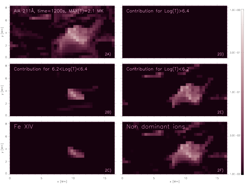
Figure 12: The synthetic 211Å image, at the AIA spatial resolution, is shown in panel 2A. The intensities $I_{I}$, $I_{D}$, $I_{H}$,$I_{L}$, $I_{ND}$ are shown in panel 2B, 2C, 2D, 2E, and 2F respectively. The color-scheme is shown in the right colorbar in logarithmic scale and all panels are normalized to the maximum of the synthesized intensity (panel 2A). All panels have the SDO/AIA spatial resolution.

The presence of small-scale structures in the emergent intensity images from our simulations, and their impact on the importance of non-dominant ions, indicates that the relatively coarse spatial resolution of AIA images could change some of our results concerning the extent to which non-dominant ions and different temperature ranges contribute to the emission in each channel (Section 3.3). In order to asses this effect, we degraded the synthesized intensities to the AIA spatial resolution. Figure 12 and Movie 4 show the same plots as shown in Figures 7 and 9, and Movies 1 and 3 but at the AIA spatial resolution. In the same manner as in the previous sections we show here one example (Figure 12), but the online Movie 4 shows the same panels for all channels and at the three different instants ($t=[880,1200,1460]$ s). In Figure 12, the synthesized 211 Å image at the SDO/AIA spatial resolution at time 1200 s is shown in the panel labeled 2A. The emission from the temperatures between $6.2<\log(T)<6.4$ ($I_{I}$) is shown in panel 2B. The emission from the dominant ion (Fe XIV, $I_{D}$) is shown in panel 2C. The emission from temperatures higher than $\log(T)=6.4$ for the 211 Å channel ($I_{H}$) is shown in panel 2D. The emission from temperatures smaller than $\log(T)=6.2$ ($I_{L}$) is shown in panels 2E. Finally, the emission from the non-dominant ions ($I_{ND}$) is shown in the panel 2F. All of these images are at the SDO/AIA spatial resolution. See Movie 4 for all the channels and all three instants, the layout is the same as in the figure.

In general, the detailed descriptions given in section 3.3 are also valid when the synthesized intensities are convolved and pixelized to the SDO/AIA resolution. However, the smaller structures disappear or are mixed with emission coming from other structures.

A.1 94, 193 and 211 Å channels

The 94, 193, 211 Å channels show strong contributions from so-called non-dominant ions ($I_{ND}$, panels 1-3F in Movie 4): most features seen in the emission from the dominant ion(s) ($I_{D}$, panels 1-3C in Movie 4) are different, both in shape and intensity, compared to the synthesized total intensity (panels 1-3A in Movie 4). As mentioned in Section 3.3, most of the emission comes from plasma cooler than the formation temperatures of the dominant ion ($I_{L}$, see panels 1-3B). It is also important to note that the structures seen in the intensity images at the SDO/AIA resolution appear very different for the various temperature ranges (compare to panels 1-3B, 1-3D and 1-3E). The reason for this is that, for these channels, the source of the emission for the various temperature ranges comes from physically distinct features or regions. This is also noted and described in the previous sections and is clearly seen in the full resolution Movies 1 and 3.

A.2 131, 171 and 304 Å channels

When taking into account the SDO/AIA resolution, most of the emission for the 131 Å, 171 Å, and 304 Å channels comes from the dominant ion(s) ($I_{D}$, panels 1-3C in Movie 4), and in only a few places do we find that the intensity changes ($I_{T}$) due to a small contribution coming from the non-dominant ions ($I_{ND}$, see panels 1-3F in Movie 4). Therefore, at all three instants, most of the emission comes from temperatures near the formation temperature of the dominant ion(s) ($I_{L}$, see panels 1-3B in Movie 4). The emission from the hot ($I_{H}$, see panels 1-3D) and the cold plasma ($I_{L}$, see panels 1-3E) are almost negligible at all instants and almost everywhere. Taking into account the SDO/AIA resolution, the temperature dependence and the contribution of the different ions, we find that the results discussed in Section 3.3 do not change considerably.

A.3 335 Å channel

As mentioned previously, the model does not reach temperatures representative of strong active regions or flares. Most of the emission in this channel is thus from lines coming from the non-dominant ions that form at temperatures lower than the dominant ion ($I_{ND}$, see panels 1-3F in Movie 4). Therefore, most of the emission comes from plasma at temperatures lower than the formation temperature of the dominant ion ($I_{L}$, see panels 1-3E in Movie 4). Once again, the results at the SDO/AIA spatial resolution do not differ significantly from the description given in Section 3.3 which are at the full model resolution.

Appendix B Abundances: coronal or photospheric?

The intensity of the various strong lines in each AIA passband can be significantly affected by the assumed values for the element abundances, which are in turn also important to interpret the observational data. In order to investigate the effect of the chemical composition we synthesized AIA observations for two different sets of abundances: photospheric abundances (Grevesse & Sauval 1998), and coronal abundances (Feldman 1992). Element abundances in solar coronal plasmas often depart from their photospheric values, and these abundance anomalies appear to correlate with the element’s First Ionization Potential (FIP). Low FIP elements ($<10$ eV; e.g., Fe, Mg, Si) are found to be enhanced in the corona typically by a factor $\sim 3-4$, and high FIP elements ($\gtrsim 10$ eV; e.g., O, Ne) have coronal abundances close to their photospheric values (see e.g., reviews by Meyer 1985; Feldman 1992). A set of “coronal abundances” compiled by (Feldman 1992) is often used for studies of coronal emission - and is assumed in the calculations for the standard temperature responses of the AIA EUV channels - although detailed studies of the chemical composition of solar plasmas have shown that this “FIP effect” varies in different types of solar features (with, e.g., coronal holes, fast solar wind, and newly emerged active regions showing abundances close to photospheric), from structure to structure, and in time (see e.g., Testa 2010 for a brief review).

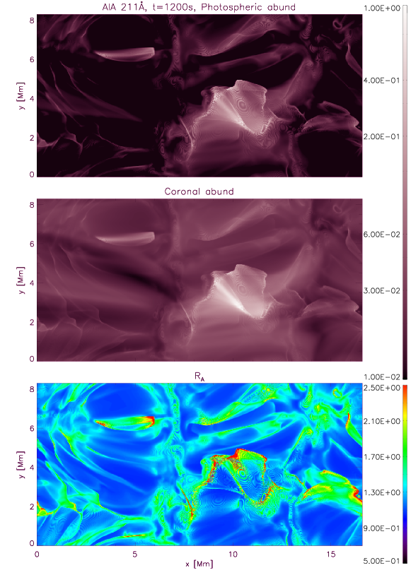
Figure 13: A comparison of the 211 Å intensity, at time 1200 s, using photospheric (top panel) and coronal (middle panel) abundances. The color-scheme is shown in the top-right colorbar using logarithmic scale. The $R_{A}$ term (see Equation B1) is shown in the bottom panel. The color-scheme is shown in the bottom-right colorbar.

As in the previous sections, we here show one example (the 211Å channel; Figure 13), and refer the reader to the online Movie 5 which shows the results for all the channels, and at the three different instants ($t=[880,1200,1460]$ s). Figure 13 shows the synthesized 211 Å image at time 1200 s using photospheric abundances (top panel) or coronal abundances (middle panel). The bottom panel shows the term $R_{A}$ which is defined as:

$$R_{A}=\left(\frac{I_{TPh}}{I_{TCo}}\right)\left(\frac{A_{DCo}}{A_{DPh}}\right)$$ (B1)

where $A_{DPh}$, and $A_{DCo}$ are the photospheric abundance, and the coronal abundance of the dominant ion (see last column in Table 1). $R_{A}$ is therefore close to 1 where the dominant ion really dominates the emission. $R_{A}$ is significantly different from 1 where there is significant contribution to the emission from non-dominant ions of elements that have relative abundances in the two datasets different from the element emitting the dominant line. We note that, for all the AIA EUV channels, the dominant line(s) are produced by Fe  ions, at various ionization stages, except for the 304 Å channel which is dominated by emission from He II. In the previous sections we used the photospheric abundance (Grevesse & Sauval 1998).

B.1 94, 171 Å channels

For the 94, and 171 Å channels the synthetic intensity calculated with the photospheric abundances is, in most areas and at all instants, about 3.8 times smaller than the intensity calculated with the coronal abundances. $R_{A}$ is close to 1 (dark blue color in Figure 13 and Movie 5), reflecting the differences between the two datasets in the abundance of Fe, which generally dominates the emission in these channels (see Table 1). In the 171 channel, the limited areas where $R_{A}$ significantly departs from 1 (and is up to 2.9) correspond to small and narrow features, where the relative contribution of emission from elements other than Fe is substantial. These large $R_{A}$ values are due to ions of elements with high first ionization potential (FIP), such as O V/VI, and Ne IV/V.

B.2 193, 211, and 335 Å channels

For the 193, 211, and 335 Å channels the difference of the synthetic images assuming photospheric or coronal abundances is twofold. We find that these channels show large regions where the $R_{A}$ varies rather smoothly between $1-1.7$, $1.2-2$ and $1.2-1.5$ for the 193, 211, and 335 Å channels respectively (Figure 13 and Movie 5). This is because these channels contain significant contributions from non-Fe ions throughout the field of view (as shown in the above).

In addition, there are also small and narrow features where $R_{A}$ significantly departs from 1. These are regions where the relative contribution of emission from elements other than Fe is very substantial. This is similar to the very narrow features seen in the 171 Å channel. In the 193, 211, and 335 Å channels $R_{A}$ is as high as 2.9, 3.2, and 3.4 respectively. These large $R_{A}$ values are due to ions of elements with high first ionization potential (FIP), such as O V/VI, and Ne IV/V. In the case of channels 211 and 335 Å, we observe significant variability in time, e.g. with the maximum $R_{A}$ value going down to 2.9 and 2.3 at time 1200 and 1460 s respectively. This is because, at later times in the evolution the atmosphere is hotter (t=1460 s) and the relative contribution of O  ions is smaller.

B.3 131, and 304 Å channels

For the 131 Å channel, at all instants, the intensity calculated with the photospheric abundances is between 2.5 and 3.3 times smaller than the intensity calculated with the coronal abundances (see Movie 5). We note that $R_{A}$ does not reach values close to 1 at any location and time. The reason is that in this channel the contribution of the high FIP elements O and Ne to the total emission is important, and the emission of these non-dominant ions (O VI, and Ne VI/VII) have characteristic temperatures of formation similar to the dominant ion, Fe VIII. So the temperature dependence of the relative contribution of the different elements is less pronounced in the 131 Å channel than in the other channels.

Finally, for the 304 Å channel, at all three instants, the intensity calculated assuming photospheric abundances ranges from 0.4 to 1 times the intensity calculated using coronal abundances (see Movie 5). Values significantly lower than 1 are due to the contribution of Mg VIII and Si VIII/IX/XI to the emission observed in this channel.

In contrast to the 94, 171, 193, 211, and 335 Å channels, the 131 and 304 Å channels do not show evidence of the narrow features with high $R_{A}$ values. This is likely due to two reasons. The dominant ions of these channels are formed at transition region temperatures, so that emission from non-dominant ions that have the same formation temperature as the dominant ion (i.e., transition region) will form in the same narrow, transition region features as the dominant ions. As a result, $R_{A}$ maps will appear relatively flat in the spatial dimension, and lack narrow spatial features. Or alternatively, if non-dominant ions have higher formation temperatures, they will tend to form coronal features, which are typically wider and smoother in the spatial dimension (and thus in the $R_{A}$ maps).

Appendix C Electron density effects

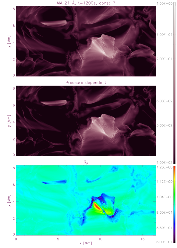
Figure 14: A comparison of the synthesized intensity considering constant pressure and taken into account the $G(T,n_{\rm e})$ for the 211 Å channel at time 1200 s are shown in the top and middle panels. The color-scheme is shown in the top-right colorbar in logarithmic scale. The ratio between the former and the later ($R_{P}$) is shown in the bottom panel. The color-scheme is shown in the bottom-right colorbar.

The line emissivities are generally a function of both temperature and pressure (or density) of the plasma. Since most lines depend to a much lesser extent on density than temperature, their emission is often computed assuming the emissivity $G(T)$, for constant pressure. Here we investigate the effect of density in the AIA EUV passbands by comparing the synthetic observations obtained from our 3D dynamic simulation using $G(T)$ and $G(T,n_{\rm e})$ (see Section 2.1 for a detailed description of the methods to calculated synthetic emission). In the same manner as the previous section we show here one example (Figure 14) and refer the reader to the online Movie 6. Figure 14 shows the synthesized 211 Å emission using $G(T)$ (for $P_{\rm e}=10^{15}$ cm^-3 K; top panel), or $G(T,n_{\rm e})$ (middle panel), and their ratio, $R_{P}$, in the bottom panel. In the previous sections, as noted, we have used $G(T,n_{\rm e})$.

C.1 131, and 335 Å channels

It is interesting to observe that the ratio $R_{P}$ does not show significant departures from 1 in the 131 and 335 Å channels, indicating that the lines contributing to the emission in these channels are not density sensitive. For instance, the most important lines in channel 335 Å are not density sensitive. In contrast, channel 131 Å has two rather important spectral lines which are density sensitive: Fe VIII 130 Å and Fe VIII 131 Å. However, the dependence with the density is in opposite directions, and as a result the channel is not particularly sensitive to the density.

C.2 94, 171, 193, 211, and 304 Å channels

In the 94, 171, 193, and 211 Åchannels, $R_{P}$ has values different from 1 in a few structures, especially at later times (t=1200 and 1460 s). Some of these features are common to all these channels, such as the strong emergent loop in the center of the field of view at time 1200 s. However, $R_{P}$ has different values in different regions for each channel. For instance, in channel 94 Å, $R_{P}$ is larger ($R_{P}\approx 1.4$) in the center of the emergent structure. In the surroundings of this region, $R_{P}$ decreases slowly until it gets near to 1. In channel 193 Å, $R_{P}$ is maximum in the left side of this emergent structure and below 1 at the boundaries of this structure. However, other features observed in the $R_{P}$ maps appear in some channels but not in others. This can be easily seen in the bottom part of the image at time 1460 s (in red) in the 211 Å channel), which is not visible in the other channels.

This difference between the channels indicates that various lines which are density sensitive contribute considerably to these channels. The 94 Å channel has one spectral line which is rather strongly influenced by the density and contributes considerably to the emission, i.e., Fe X 94 Å. The 171 Å channel has a strong contribution from the spectral line Fe IX 171 Å which has some dependence on the density. In addition, other lines which contribute less to the emission have stronger dependence with the density, i.e., Fe X 170 Å, O V 171 Å, and Ni XIV 171 Å. The 193 Å channel has several spectral lines which contribute to the emission and are density dependent, i.e., several spectral lines coming from Fe XII within the range of wavelength 186-191 Å, O V 192 Å, Fe X 193 Å, Fe XI 188 Å and several spectral lines coming from Fe IX within the range of wavelength 182-189 Å. The 211 Å channel has some spectral lines which contribute to the emission and are strongly density dependent, i.e., O V 215 Å, Fe XIV 211 Å, O IV 208 Å, Fe XIII 202 Å, Fe XII 211 Å, and Fe X 207 Å. Finally, the 304 Å channel has faint contributions from a few spectral lines that are strongly density dependent: Si VIII 316 Å, and N IV 332 Å. Therefore, since all of these channels show various spectral lines which have density dependence, the $R_{P}$ maps shows values that are different from 1 in different regions.

Figure 5: Histogram of coronal temperatures of the model at t=[800, 1200, 1460] s, shown with solid, dotted and dashed lines respectively. The histogram is for temperatures larger than 30,000 K. The snapshots are representative of solar conditions in a coronal hole (800 s) and quiet Sun with small hotter emerging regions (1200 s) and with hotter corona (1460 s).

Table 1: Synthesized SDO/AIA channels

SDO/AIA channel	Dominant ion(s)	Temperature	Cor/phot abund
94 Å	Fe X/XVIII	$10^{6}/6\,10^{6}$ K	3.981
131 Å	Fe VIII/XX	$6.\,10^{5}/10^{7}$ K	3.981
171 Å	Fe IX/X	$7.\,10^{5}/10^{6}$ K	3.981
193 Å	Fe XII/XXIV	$1.2\,10^{6}/2.\,10^{7}$ K	3.981
211 Å	Fe XIV	$2\,10^{6}$ K	3.981
304 Å	He II	$10^{5}$ K	0.933
335 Å	Fe XVI	$2.5\,10^{6}$ K	3.981

Note. — The synthesized SDO/AIA channels in this work are listed in the first column. The dominant ion(s) for each channel, the formation temperature(s) of the dominant ion(s) and the ratio between the abundance of the dominant ion(s) assuming the coronal datasets and photospheric datasets are listed in the second, third, and fourth columns.

Table 2: Selection of $y$-possitions Movie 2

plot in movie 2	style and color	criteria
1-3a	solid red	$(I_{NDL}/I_{D})I_{T}$
1-3b	dashed red	$I_{NDL}/I_{D}$
1-3c	solid green	$(I_{NDH}/I_{D})I_{T}$
1-3d	dashed green	$I_{NDH}/I_{D}$

Note. — Each panel (labels listed in the first column of this table) in Movie 2 shows results for a different $y$-position in the field of view. These locations are marked with crosshairs in the panels 1-3D in Movie 1, the color and style of each crosshair is given in the second column of this table. The chosen locations are such that the criterium listed in the third column of this table is maximized.

References

- Aschwanden & Boerner (2011) Aschwanden M. J., Boerner P., 2011, ApJ, 732, 81
- Berger et al. (2011) Berger T., Testa P., Hillier A., et al., 2011, Nature, 472, 197
- De Pontieu et al. (2007) De Pontieu B., Hansteen V. H., Rouppe van der Voort L., van Noort M., Carlsson M., 2007, ApJ, 655, 624
- De Pontieu et al. (2011) De Pontieu B., McIntosh S. W., Carlsson M., et al., 2011, Science, 331, 55
- Dere et al. (2009) Dere K. P., Landi E., Young P. R., et al., 2009, A&A, 498, 915
- Feldman (1992) Feldman U., 1992, Phys. Scr, 46, 202
- Feldman et al. (2010) Feldman U., Ralchenko Y., Doschek G. A., 2010, ApJ, 708, 244
- Grevesse & Sauval (1998) Grevesse N., Sauval A. J., 1998, Space Sci. Rev., 85, 161
- Gudiksen et al. (2011) Gudiksen B. V., Carlsson M., Hansteen V. H., et al., 2011, A&A, 531, A154
- Gudiksen & Nordlund (2004) Gudiksen B. V., Nordlund Å., 2004, An Ab Initio Approach to the Solar Coronal Heating Problem, en IAU Symposium, Vol. 219, Dupree A. K., Benz A. O. (eds.), Stars as Suns : Activity, Evolution and Planets, p. 488
- Hansteen et al. (2007) Hansteen V. H., Carlsson M., Gudiksen B., 2007, 3D Numerical Models of the Chromosphere, Transition Region, and Corona, en Astronomical Society of the Pacific Conference Series, Vol. 368, Heinzel P., Dorotovič I., Rutten R. J. (eds.), The Physics of Chromospheric Plasmas, p. 107
- Hansteen et al. (2006) Hansteen V. H., De Pontieu B., Rouppe van der Voort L., van Noort M., Carlsson M., 2006, Apj, 647, L73
- Hansteen et al. (2010) Hansteen V. H., Hara H., De Pontieu B., Carlsson M., 2010, ApJ, 718, 1070
- Heggland et al. (2009) Heggland L., De Pontieu B., Hansteen V. H., 2009, ApJ, 702, 1
- Krishna Prasad et al. (2011) Krishna Prasad S., Banerjee D., Gupta G. R., 2011, A&A, 528, L4
- Madjarska et al. (2011) Madjarska, M. S., Vanninathan, K., & Doyle, J. G. 2011, A&A, 532, L1
- Martínez-Sykora et al. (2011) Martínez-Sykora J., De Pontieu B., Hansteen V., McIntosh S. W., 2011, ApJ, 732, 84
- Martínez-Sykora et al. (2008) Martínez-Sykora J., Hansteen V., Carlsson M., 2008, ApJ, 679, 871
- Martínez-Sykora et al. (2009) Martínez-Sykora J., Hansteen V., Carlsson M., 2009, ApJ, 702, 129
- Martínez-Sykora et al. (2009) Martínez-Sykora J., Hansteen V., DePontieu B., Carlsson M., 2009, ApJ, 701, 1569
- Martínez-Sykora et al. (2011) Martínez-Sykora J., Hansteen V., Moreno-Insertis F., 2011, ApJ, 736, 9
- Meyer (1985) Meyer J.-P., 1985, ApJS, 57, 151
- O’Dwyer et al. (2010) O’Dwyer B., Del Zanna G., Mason H. E., Weber M. A., Tripathi D., 2010, A&A, 521, A21
- Rouppe van der Voort et al. (2009) Rouppe van der Voort L., Leenaarts J., de Pontieu B., Carlsson M., Vissers G., 2009, ApJ, 705, 272
- Schmelz et al. (2011) Schmelz J. T., Jenkins B. S., Worley B. T., et al., 2011, ApJ, 731, 49
- Testa (2010) Testa P., 2010, Space Sci. Rev., 157, 37
- Testa et al. (2011) Testa P., Drake, Landi, 2011, submited to ApJ
- Foster et al. (2011) Foster, Testa P., 2011, submited to ApJL