LTE model atmopsheres
MARCS, ATLAS and CO5BOLD

Abstract

In this talk we review the basic assumptions and physics covered by classical 1D LTE model atmospheres. We will focus on ATLAS and MARCS models of F-G-K stars and describe what resources are available through the web, both in terms of codes and model-atmosphere grids. We describe the advances made in hydrodynamical simulations of convective stellar atmospheres with the CO⁵BOLD code and what grids and resources are available, with a prospect of what will be available in the near future.

1 Introduction

A model atmosphere is a numerical model that describes the physical state of the plasma in the outer layers of a star, and is used to compute observable quantities, such as the emerging spectrum or colours. Different degrees of complexity lead to different classes of models. The first simplification that is made in the models we shall describe is that of Local Thermodynamic Equilibrium (LTE). Although we know that a stellar atmosphere cannot be in thermodynamic equilibrium, since we see that radiation is escaping in open space, we make the assumption that locally we are very close to thermodynamic equilibrium. In practice this means that we assume that at each point in the atmosphere, which we identify by some suitable coordinates $X,Y,Z$ and in a volume $\Delta X\Delta Y\Delta Z$ around it, we can define a temperature T. This temperature can be used to describe the velocity distribution of the particles, that will be a Maxwellian distribution, to compute the occupation numbers of the atomic levels of the different species, through Boltzmann’s law and the ionisation equilibria through Saha’s law. The LTE hypothesis greately simplifies the computation of model atmospheres, by providing us a quick and easy way to compute all the micro-physics of the plasma, just by knowing the temperature (and gas pressure) at any given point.

The next simplification concerns the dimensionality of the problem. Do we really need to treat this as a three-dimensional problem ? If we simplify our model by assuming that the atmosphere is homogeneous in two directions and shows variations of the physical quantities only along one direction (vertical, for plane-parallal atmosheres, radial for spherical atmospheres), we have reduced our problem to one dimension.

In principle all the physical quantities in the plasma may change with time. A simplification is to assume that the atmosphere is stationary and then the problem becomes time-independent.

All these simplifications are adopted in the widely used MARCS and ATLAS model atmospheres. In spite of what can appear at first sight as an oversimplification, these model atmospheres are capable of reproducing a wide range of observable quantities and have a high predictive power.

The CO⁵BOLD model atmospheres make the hypothesis of LTE, however are fully three dimensional (two dimensional models may also be computed) and time-dependent. In this respect they are more realistic, since they can describe effects that cannot be accounted for by 1D models. This extra realism, however comes at a price and we shall discuss this later.

In the following we shall give only a very sketchy description of the basic principles that are at the basis for the computation of model atmospheres, since these are well described in the relevant publications. We shall instead try to adopt an ”end user” approach pointing out how such tools can be used and what resources are available.

2 ATLAS and MARCS

2.1 Basic principles

Both the ATLAS [Kurucz(1970), Kurucz(1993), Kurucz(2005), (Kurucz 1970,1993,2005)] and MARCS [Gustafsson et al.(1975), Plez et al.(1992), Edvardsson et al.(1993), Asplund et al.(1997), Gustafsson et al.(2003), Gustafsson et al.(2008), (Gustafson et al. 1975; Plez et al. 1992; Edvardssoon et al. 1993; Asplund et al. 1997; Gustafsson et al. 2003,2008)] models are one dimensional and static. MARCS can deal either with plane-parallel or spherical geometry, ATLAS only with plane-parallel, although SATLAS [Lester & Neilson(2008), (Lester & Neilson 2008)] can compute spherical models. Elswhere in this volume Neilson [Neilson, (2011)] talks about SATLAS and spherical models. In what follows we shall assume plane-parallel geometry for both MARCS and ATLAS.

Both codes assume that the atmosphere is in hydrostatic equilibrium, this provides the first basic equation necessary to compute a model atmosphere. The equation of hydrostatic equilibrium states that the gas pressure gradient is balanced by the difference between gravity and the sum of turbulent pressure gradient and radiative acceleration. In MARCS the turbulent pressure gradient is treated defining an “effective gravity” $g_{\rm eff}$, see [gustfsson08, Gustafsson et al. (2008)]. In ATLAS there is an explicit term for the turbulent pressure, proportional to density and the square of turbulent velocity. The equation of hydrostatic equilibrium must be coupled with the equation of radiative transfer, and the condition of energy conservation. The atmosphere simply transports the energy, there is no net absorption or creation of energy within the atmosphere. A convenient variable is the mass column density $dm=-\rho dx$, RHOX (pronounced “rocks” for those who like reading the FORTRAN). The goal of the model atmosphere computation is to define the run of the temperature $T(m)$, and the energy conservation provides a mean to modify a trial value of $T$ in order to satisfy the condition. The global parameters that define the model are the surface gravity $g$, the energy/surface = integral of flux over all frequencies = $\sigma\rm T_{eff}^{4}$, where the latter can be taken as a definition of “effective temperature” and the “chemical composition”, that affects the opacities and the equation of state. At each step in the computation the hypothesis of LTE allows to compute occupation numbers and ionization fractions that allow to compute the opacity. ATLAS has two ways of dealing with line opacities, either through the Opacity Distribution Functions (ODFs, version 9 of ATLAS) or through Opacity Sampling (version 12 of ATLAS). Early versions of MARCS also used ODFs, but the currently used version is OSMARCS, that uses opacity sampling. We stress that tests conducted with ATLAS 9 and ATLAS 12 show that the differences between a model computed with ODFs and one computed with Opacity Sampling are minor and can be ignored for all practical purposes. The choice on whether to use ATLAS 9 or ATLAS 12 is a matter of convenience, if a large number of models needs to be computed with the same chemical composition, then ATLAS 9 is the obvious choice. If several models with slightly different chemical composition are required, ATLAS 12 is more handy.

In the atmospheres of cool stars, a complication is that in the deep layers energy is mainly transported by convection. Both MARCS and ATLAS use a “mixing length” approximation. However MARCS uses the [Henyey, Vardya, & Bodenheimer(1965), Henyey et al. (1965)] formulation, while ATLAS uses essentially the [Mihalas(1970), Mihalas (1970)] formulation, in a way that is detailed by [Castelli, Gratton, & Kurucz(1997), Castelli, Gratton & Kurucz (1997)]. At large optical depths where convection dominates, a consequence is that a MARCS and an ATLAS model will be slightly different, even if they have been computed with the same mixing length parameter $\alpha_{\mathrm{MLT}}$. The effect is illustrated in [Bonifacio et al.(2009), Bonifacio et al. (2009)], appendix A, figure A.2. We wish to give here a warning: ATLAS has an option for an “approximate treatment of overshooting”, well described by [Castelli, Gratton, & Kurucz(1997), Castelli et al. (1997)], that we recommend users to switch off. This is also the recommendation of [Castelli, Gratton, & Kurucz(1997), Castelli et al. (1997)], but in our view the most convincing reason is that this option produces a temperature structure that is inconsistent with the mean temperature structure of hydrodynamical simulations.

2.2 Availability

The ATLAS code has always been distributed publicly, on an “as is” basis and a “do not use blindly” clause. The main site is Kurucz’s site kurucz.harvard.edu were you can find all the source codes of versions 9 and 12 of ATLAS, as well as the spectrum synthesis suite SYNTHE, the abundance analisis code WIDTH and a lot more. We call attention to a code called binary that allows to combine two synthetic spectra to sythesise the spectrum of an SB2 binary. The site also contains a large choice of ODFs, atomic data to compute new ODFs, atomic and molecular data for spectrum synthesis. There is also a large grid of computed ATLAS 9 models, that can be used “off the shelf”.

One difficulty faced by ATLAS users is that Kurucz uses DEC computers running under the VMS operating system. While such systems were widely spread in the eighties, and still existent in the ninties, the majority of researchers has access to Unix work stations, and a large fraction are Linux systems. [SB04, Sbordone et al. (2004)] presented a port of ATLAS and the other codes for Linux, see also [SB05, Sbordone (2005)].

Fiorella Castelli is very active in updating and improving the codes, the latest version of the Linux version of the codes can always be found on her web site wwwuser.oats.inaf.it/castelli. On the site you can also find a large grid of computed ATLAS 9 models and fluxes, as well as ODFs to compute further models you might need.

With Luca Sbordone and Fiorella Castelli we also provided a site were the codes are nicely bound in tar-balls and come with a Makefile that allows an easy installation. The site attempts also to collect available documentation and example scripts to run the various programmes, to provide a starting point for beginners. The site was initially hosted by the Trieste Observatory, but has now moved to the Paris Observatory atmos.obspm.fr. We try to keep the source codes always aligned with those on the site of Fiorella Castelli.

For users of ATLAS and related codes there are discussion and announcement lists that are mantained at the University of Ljubljana:
list.fmf.uni-lj.si/mailman/listinfo/kurucz-discuss.

The MARCS code is not publicly available, so if you need a particular MARCS model you have to ask one of its developers. However there is a web site on which a large grid of computed models and fluxes is publicly available: marcs.astro.uu.se. You must register to the site, but registration is free. You find both plane-parallel and spherical models, as well as programs to read the models and interpolate in the grid. If you use a spherical model, make sure that the spectrum synthesis code you use is capable of properly treating the spherical transfer. For example SYNTHE is not capable of doing it, it will nevertheless run happily interpeting the spherical model as if it were plane-paralle, which is inconsistent. The turbospectrum code by B. Plez [Alvarez & Plez(1998), Alvarez & Plez (1998)] is capable of treating correctly both spherical and plane-parallel models.

Both ATLAS and MARCS are “state of the art” 1D model atmosheres. In the range of F-G-K stars the differences between the two kinds of models are immaterial, as shown e.g. in [Bonifacio et al.(2009), Bonifacio et al. (2009)]. For the very cool models (below 3750 K) MARCS models are probably more reliable, because all the relevant molecular opacities are included. ATLAS can compute models also for A-B-O stars, although for stars hotter than 20 000 K the hypothesis of LTE clearly becomes questionable. MARCS only computes models up to 8000 K, therefore if you are dealing with A-F stars, ATLAS is preferable.

3 CO⁵BOLD models

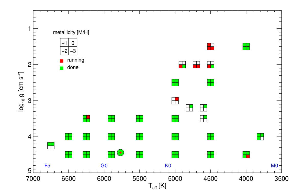
Figure 1: The current status of the CIFIST grid. This is an update of the figure shown by [Ludwig et al.(2009), Ludwig et al. (2009)] Symbols mark the location of a model in the $T_{\mathrm{eff}}$-$\log g$-plane. Green (gray) color indicates completed model runs, red (black) ongoing calculations. Each square is split into four sub-squares indicating solar, 1/10, 1/100, and 1/1000 of solar metallicity. The solar position is indicated by the round symbol. In addition to the models shown in this plot there are a few low gravity models that are beeing computed in Vilnius by Arunas Kučinskas and his collaborators.

CO⁵BOLD stands for COnservative COde for the COmputation of COmpressible COnvection in a BOx of L Dimensions with l=2,3 and is developed by B. Freytag and M. Steffen with contributions of H.-G. Ludwig, W. Schaffenberger, O. Steiner, and S. Wedemeyer-Böhm [Freytag, Steffen, & Dorch(2002), Freytag et al. (2011), (Freytag et al. 2002, 2011)].

What it does is to solve the time-dependent equations of compressible hydrodynamics in an external gravity field coupled with the non-local frequency-dependent radiation transport. It can operate in two modes: 1) the “box-in-a-star” mode, in which the computational domain covers a small portion of the stellar surface; 2) the “star-in-a-box” mode, in which the computational domain includes the whole convective envelope of a star.

The need to go to the hydrodynamical model is obvious: all the phenomena that are linked to the motions in the stellar atmospheres, like line-shifts, line asymmetries, micro-variability etc. cannot be described by 1D static models like MARCS or ATLAS.

There are cases in which the use of 1D models will provide the wrong results, thus making the use of 3D models mandatory. One case is the measurement of ⁶Li in metal-poor warm dwarf stars. [Cayrel et al.(2007), Cayrel et al. (2007)] have shown that the line asymmetry due to convection can mimic the presence of up to 5% ⁶Li, thus an analysis of the spectra based on 1D model atmospheres, that provide only symmetric line profiles, will result in a ⁶Li abundance that is spurious, even if no ⁶Li is present. In fact this is a misinterpretation of the convective line asymmetry. Another case is the measurement of the abundance of thorium in the solar photosphere. The only line suitable for this purpose is the 401.9 nm Thii resonance line, that lies on the red wing of a strong blend of Ni and Fe. [Caffau et al.(2008), Caffau et al. (2008)] have shown that neglect of the line asymmetry of this Ni-Fe blend would result in an over-estimate of the Th abundance by about 0.1 dex. Another effect that is very important in metal-poor stars is the so called “overcooling” [Asplund et al.(1999), Collet et al.(2007), Caffau & Ludwig(2007), González Hernández et al.(2008), Bonifacio, Caffau, & Ludwig(2010), (Asplund et al. 1999; Collet et al. 2007; Caffau & Ludwig 2007; González Hernández et al. 2008; Bonifacio et al. 2010)]. The hydrodynamical models predict much cooler temperatures in the outer layers than do the 1D models, resulting in important differences in the computed line strength for all the lines that form in these outer layers. This is the case for all the molecular species usually used for abundance determinations [Behara et al.(2010), (Behara et al. 2009)], but also for some atomic species [Bonifacio, Caffau, & Ludwig(2010), (Bonifacio et al. 2010)].

The larger amount of information provided by the 3D models comes at a larger computational cost and the need to simplify the treatment of some physical effects. The first necessary simplification is the treatment of opacity. In the computation of an hydrodynamical model we cannot afford a treatment of opacity as detailed as we can in 1D. For this reason the opacities are grouped into a small number (less or equal to 14) of opacity bins [Nordlund (198), Ludwig (1992), Ludwig, Jordan, & Steffen(1994), Vögler, Bruls, & Schüssler (2004), (Nordlund 1982; Ludwig 1992; Ludwig et al. 1994; Voegler et al. 2004)]. Further simplifications are currently an approximate treatment of scattering in the continuum, and neglecting effects of line shifts in the evaluation of the line blocking.

3.1 The CIFIST grid

A hydrodynamical model is not easy to perform since it can need several months for dwarf stars up to more than a year for giants (on PC-like machines). Typically, one ends-up with a time series covered by about 100 snapshots representing a couple of convective turn-over times. These occupy several GB of storage space. The computational and human effort to compute an hydrodynamical model is such that we cannot expect to be able to compute a model for any set of input parameters on a working time scale of few weeks.

Furthermore, not all snapshots are statistically independent. It would thus be not wise to attempt a “brute force” approach and compute the emerging spectrum from each and every snapshot. A preferable strategy is to select a sub-sample of the snapshots that has the same global statistical properties as the total ensemble [Caffau (2009), (Caffau 2009)]. However, even selecting only 15 to 20 snapshots, the line formation computations for a large number of lines, as are usually employed in the analysis with 1D models, is computationally demanding.

For these reasons in the course of the CIFIST project (Cosmological Impact of the FIrst STars, cifist.obspm.fr) we decided to attempt the computation of a complete grid of hydrodynamical models. The foreseen use of this grid is that obseravable quantities are computed on the grid, so that they can then be conveniently interpolated for any value within the grid points. An example of this is provided in [Sbordone et al.(2010), Sbordone et al. (2010)] where a fitting function is provided to the curves of growth of the Lii doublet computed on the grid. One inputs the measured equivalent width, effective temperature, surface gravity and metallicity and the fitting function provides the lithium abundance. Another example is [JGH, Gonzàlez Hernàndez et al. (2010)] where the OH lines have been computed on the grid and the results may be used for abundance analysis.

Such ready-to-use tools are probably more useful to researchers than providing the 3D models “as is”. We are thus concentrating on computing a meaningful set of observable quantities so that the CO⁵BOLD models can be widely used for abundance analysis.

Tout Can you not get around the time taken to complete the full 3-D calculation by something like a two-stream model with large slowly rising cells and smaller rapidly falling cells?

Bonifacio No. This was the approach tried by R.L. Kurucz in ATLAS 11, a version of ATLAS that was never released for public use, and employed by him to assess the effect of granulation on the line formation of the lithium doublet in Pop II stars (Kurucz 1995, ApJ 452, 102). His result was that the Li abundance should be higher than what derived from an analysis with ATLAS 9 by almost one order of magnitude. This result is totally wrong. We now know that when treated in LTE the effect of granulation is to lower the Li abundance by 0.2 to 0.3   dex (Asplund et al. 1999 A&A 346 L17). The two stream model was certainly worth exploring, at the time it looked to me a brilliant idea. In retrospect we can see why it failed: to compute each stream in a 1D approach you have to assume energy conservation, for each stream. This condition is clearly violated and with this approach you cannot take into account the energy exchanges between the streams.

Petr Harmanec After listening to your excellent talk, I am about to commit a suicide. Do you think that the 3D model atmosphere models will get to the level that non-experts would be able to use them for a reliable comparison with real observations?

Bonifacio Indeed we hope 3D models may become of general use, we think that the most promising approach is to have a grid of 3D model atmospheres, like the CIFIST grid, and provide to users observable quantities computed across the grid and means to interpolate in between grid points. A good example is the fitting function for the Li abundance provided by Sbordone et al. (2010). I stress again that in the computation of 3D model atmospheres and associated line formation we make some simplifications. Notably line opacity and scattering are treated in more detail in a 1D computation.

A. Prša Your 3D models are computed for spherical stars. If one wanted to compute a spectrum of a distorted star, could one compute the intensities for each tile of the discretized surface and then sum them up? Bonifacio The spherical geometry is dealt with in the star-in-a-box models. It looks to me more correct to treat distorsion to sphericity directly in this kind of computation, rather than tiling several box-in-a-star models. This has never been done so far, to my knowledge. I suggest you contact B. Freytag, who has been computing many star-in-a-box CO⁵BOLD models and can answer your question more fully than myself. I am not a CO⁵BOLD developer, I am just an end user.

References

- [Alvarez & Plez(1998)] Alvarez, R., & Plez, B. 1998, A&A,330, 1109
- [Asplund et al.(1997)] Asplund, M., Gustafsson, B., Kiselman, D., & Eriksson, K. 1997, A&A, 318, 521
- [Asplund et al.(1999)] Asplund, M., Nordlund, A., Trampedach, R., Stein, R., 1999, A&A, 346, L17
- [Behara et al.(2010)] Behara, N. T., Bonifacio, P., Ludwig, H.-G., et al. 2010, A&A,513, A72
- [Bonifacio et al.(2009)] Bonifacio, P., et al. 2009, A&A,501, 519
- [Bonifacio, Caffau, & Ludwig(2010)] Bonifacio, P., Caffau, E., & Ludwig, H.-G. 2010, A&A,524, A96
- [Caffau (2009)] Caffau E., 2009 Abondances des éléments dans les soleil et dans les étoiles de type F-G-K avec des modèles hydrodynamiques d’atmosphères stellaires, thèse doctorale, Observatoire de Paris
- [Caffau & Ludwig(2007)] Caffau E., & Ludwig H.-G., 2007, A&A, 467, L11
- [Caffau et al.(2008)] Caffau, E., Sbordone, L., Ludwig, H.-G., et al., 2008, A&A,483, 591
- [Castelli, Gratton, & Kurucz(1997)] Castelli, F., Gratton, R. G., & Kurucz, R. L. 1997, A&A,318, 841
- [Cayrel et al.(2007)] Cayrel, R., et al. 2007, A&A,473, L37
- [Collet et al.(2007)] Collet, R., Asplund, M., Trampedach, R., 2007, A&A, 469, 687
- [Edvardsson et al.(1993)] Edvardsson, B., Andersen, J., Gustafsson, et al. 1993, A&A, 275, 101
- [Freytag, Steffen, & Dorch(2002)] Freytag, B., Steffen, M., & Dorch, B. 2002, Astronomische Nachrichten, 323, 213
- [Freytag et al. (2011)] Freytag, B. et al. 2011, “Realistic simulations of stellar convection”, Journal of Computational Physics: special topical issue on computational plasma physics, ed. Barry Koren
- [González Hernández et al.(2008)] González Hernández, J., Bonifacio, P., Ludwig, H.-G., et al. 2008, A&A, 480, 233
- [González Hernández et al.(2010)] González Hernández, J. I., Bonifacio, P., Ludwig, H.-G., et al. 2010, A&A,519, A46
- [Gustafsson et al.(1975)] Gustafsson, B., Bell, R. A., Eriksson, K., & Nordlund, A. 1975, A&A, 42, 407
- [Gustafsson et al.(2003)] Gustafsson, B., Edvardsson, B., Eriksson, K., et al. 2003, Stellar Atmosphere Modeling, 288, 331
- [Gustafsson et al.(2008)] Gustafsson, B., Edvardsson, B., Eriksson, K., et al. 2008, A&A,486, 951
- [Henyey, Vardya, & Bodenheimer(1965)] Henyey, L., Vardya, M. S., & Bodenheimer, P. 1965, ApJ,142, 841
- [Kurucz(1970)] Kurucz, R. L. 1970, SAO Special Report,309,
- [Kurucz(1993)] Kurucz, R. 1993, ATLAS9 Stellar Atmosphere Programs and 2 km/s grid. Kurucz CD-ROM No. 13. Cambridge, Mass.: Smithsonian Astrophysical Observatory, 1993.,13,
- [Kurucz(2005)] Kurucz, R. L. 2005, Mem. SAIt Suppl.,8, 14
- [Lester & Neilson(2008)] Lester, J. B., & Neilson, H. R. 2008, A&A,491, 633
- [Ludwig (1992)] Ludwig, H.-G. 1992, PhDT, University of Kiel
- [Ludwig, Jordan, & Steffen(1994)] Ludwig, H.-G., Jordan, S., & Steffen M. 1994, A&A, 284, 105
- [Ludwig et al.(2009)] Ludwig, H.-G., Caffau, E., Steffen, et al. 2009, Mem. Soc. Astron. It.,80, 711
- [Mihalas(1970)] Mihalas, D. 1970, Stellar Atmospheres, San Francisco: Freeman, —c1970
- [Neilson (2011)] Neilson H. 2011, this volume
- [Nordlund (198)] Nordlund, Å. 1982, A&A, 107, 1
- [Plez et al.(1992)] Plez, B., Brett, J. M., & Nordlund, A. 1992, A&A, 256, 551
- [Sbordone(2005)] Sbordone, L. 2005, Mem. SAIt Suppl.,8, 61
- [Sbordone, Bonifacio, Castelli, & Kurucz(2004)] Sbordone, L., Bonifacio, P., Castelli, F., & Kurucz, R. L. 2004, Mem. SAIt Suppl.,5, 93
- [Sbordone et al.(2010)] Sbordone, L., et al. 2010, A&A,522, A26
- [Vögler, Bruls, & Schüssler (2004)] Vögler, A., Bruls, J. H. M. J., & Schüssler, M. 2004, A&A, 421, 741